Deep hard X-ray source counts from a fluctuation analysis of ASCA SIS images

Abstract

An analysis of the spatial fluctuations in 15 deep ASCA SIS0 images has been conducted in order to probe the 2-10 keV X-ray source counts down to a flux limit $\sim 2\times 10^{-14}{\rm erg}\,{\rm cm}^{-2}\,{\rm s}^{-1}$. Special care has been taken in modelling the fluctuations in terms of the sensitivity maps of every one of the 16 regions ($5.6\times 5.6\,{\rm arcmin}^{2}$ each) in which the SIS0 has been divided, by means of raytracing simulations with improved optical constants in the X-ray telescope. The very extended ‘side lobes’ (extending up to a couple of degrees) exhibited by these sensitivity maps make our analysis sensitive to both faint on-axis sources and brighter off-axis ones, the former being dominant. The source counts in the range $(2-12)\times 10^{-14}{\rm erg}\,{\rm cm}^{-2}\,{\rm s}^{-1}$ are found to be close to a euclidean form which extrapolates well to previous results from higher fluxes and in reasonable agreement with some recent ASCA surveys. However, our results disagree with the deep survey counts by Georgantopoulos et al. (1997). The possibility that the source counts flatten to a subeuclidean form, as is observed at soft energies in ROSAT data, is only weakly constrained to happen at a flux $<1.8\times 10^{-12}{\rm erg}\,{\rm cm}^{-2}\,{\rm s}^{-1}$ (90 per cent confidence). Down to the sensitivity limit of our analysis, the integrated contribution of the sources whose imprint is seen in the fluctuations amounts to $\sim 35\pm 13$ per cent of the extragalactic 2-10 keV X-ray background.

1 Introduction

In the soft X-ray band (0.5-2 keV), a combination of direct source counts in shallow and deep surveys (Hasinger et al 1993, Branduardi-Raymont et al 1994) and analyses of the spatial fluctuations (Hasinger et al 1993, Barcons et al 1994) has determined the source counts down to a level where more than 70 per cent of the extragalactic X-ray background (XRB) is resolved into sources. The most remarkable feature of the soft X-ray source counts is the existence of a break at a 0.5-2 keV flux of $2\times 10^{-14}{\rm erg}\,{\rm cm}^{-2}\,{\rm s}^{-1}$ below which the approximate euclidean behaviour that holds at brighter fluxes flattens considerably. The reason for this flattening in the source counts is the steep evolution of the broad-line Active Galactic Nuclei (AGN) which stops at redshift $z\sim 2$. The so-called Narrow-Line X-ray Galaxies (NLXGs), which might in fact be powered by obscured AGN, appear in increasingly large numbers at fluxes $\ll 10^{-14}{\rm erg}\,{\rm cm}^{-2}\,{\rm s}^{-1}$ (McHardy et al 1997, Romero-Colmenero et al 1996, Almaini et al 1996). In a recent study Hasinger et al (1997) and Schmidt et al (1997) have cast some doubts on the reality of these NLXGs, since in their complete identification of the sources found in the Lockman Hole above a flux of $5\times 10^{-15}{\rm erg}\,{\rm cm}^{-2}\,{\rm s}^{-1}$ no such objects appear. Moreover, Hasinger et al (1997) also discuss the severe confusion problems for deep surveys carried out with the ROSAT Position Sensitive Proportional Counter below that flux (where most of the NLXGs are found by other surveys). Although this might certainly affect some of the source identifications at very faint levels, the X-ray sources putatively identified as NLXGs have harder spectra than the broad-line AGN (Almaini et al 1996, Romero-Colmenero et al 1996). This indicates that regardless of their optical counterparts, these sources might be relevant to higher energies.

At harder X-ray energies (2-10 keV), where a larger fraction of the energy of the XRB resides (see, e.g., Fabian & Barcons 1992), our knowledge of the X-ray source counts is more limited. Until ASCA became operational, all the data in that energy band was collected by collimated field-of-view proportional counters with angular resolution of degrees. The Piccinotti et al (1982) sample was the only really complete sample of hard X-ray sources going down to 2-10 keV fluxes of $3\times 10^{-11}{\rm erg}\,{\rm cm}^{-2}\,{\rm s}^{-1}$. Below that flux, a GINGA high galactic latitude survey (Kondo 1991) and the GINGA fluctuation analysis (Butcher et al 1997, Hayashida 1989) extended the euclidean source counts found in the Piccinotti et al sample down to a flux of $5\times 10^{-13}{\rm erg}\,{\rm cm}^{-2}\,{\rm s}^{-1}$. The surface density reached by these studies amounted to a few sources per square degree to be compared with the deepest source counts in the soft band reaching about 1000 sources per square degree.

Even with its limited angular resolution, ASCA (Tanaka, Inoue & Holt 1994) has opened the possibility of making a very significant step forward towards the determination of the 2-10 keV source counts at faint fluxes. Various surveys have been carried out which show that the source counts do not deviate dramatically from an euclidean extrapolation of the source counts at higher fluxes. Among those surveys, the Large Sky Survey (LSS, Inoue et al 1996, Ueda 1995) covers 6 $\deg^{2}$ with the GIS down to a flux limit of $1.5\times 10^{-13}{\rm erg}\,{\rm cm}^{-2}\,{\rm s}^{-1}$ for direct source detection. The Deep Sky Survey (DSS, Inoue et al 1996) and the ASCA follow-up of 3 deep ROSAT fields by Georgantopoulos et al (1997) provide rather discrepant source counts down to fluxes of $4\times 10^{-14}{\rm erg}\,{\rm cm}^{-2}\,{\rm s}^{-1}$ and $5\times 10^{-14}{\rm erg}\,{\rm cm}^{-2}\,{\rm s}^{-1}$ respectively. Indeed, the small solid angle sampled by the deepest surveys results in significantly large statistical uncertainties in the number of sources detected down to the completeness flux. Other effects, like inhomogeneities in the distribution of sources or X-ray variability of the sources (see Barcons, Fabian & Carrera 1997 for a discussion on the effects of this last issue on the source counts) can also affect estimates of source counts when only a small area of the sky is covered.

The analysis of the spatial fluctuations in the XRB has been often used to both improve on the surveyed area and eventually to determine the source counts down to fainter fluxes than can be achieved via direct source counting. Examples of the application of this method in X-ray imaging data can be found in Hamilton & Helfand (1987), Barcons & Fabian (1990), Hasinger et al (1993) and Barcons et al (1994) among others. These analyses have either predicted or confirmed the source counts at faint fluxes with success. The theoretical sensitivity limit of this method corresponds to a flux level for which there is about one source per beam, although in some cases photon counting noise prevents that limit being reached.

In this paper we present a first fluctuation analysis of 15 high galactic latitude deep pointings obtained with the SIS0 detector on ASCA. Down to the sensitivity level of our analysis ($\sim 2\times 10^{-14}{\rm erg}\,{\rm cm}^{-2}\,{\rm s}^{-1}$) we find no compelling evidence for a flattening in the source counts. We also find our results (which cover a nominal area of 2 $\deg^{2}$) to be consistent with the LSS and the DSS within $1\sigma$ uncertainties. The Georgantopoulos et al (1997) survey, however, appears to be above our estimate of the source counts at $5\times 10^{-14}{\rm erg}\,{\rm cm}^{-2}\,{\rm s}^{-1}$ by more than 3 sigma.

In section 2 we present the data, taken from the archive, which has been used in the current analysis. Section 3 is devoted to explain how the distribution of spatial fluctuations is modelled with special emphasis on the sensitivity maps for each pixel and other effects. Section 4 presents the results of the fits to the distribution of fluctuations and the implications for source counts. In section 5 we summarize our results and discuss briefly possible extensions of this work.

2 The Data

Our data sample has been built by using all the public ASCA images in the archive which comply with a list of selection criteria. These are: galactic latitude in excess of $20\deg$ (to avoid the effects of galactic absorbing columns close to $10^{21}\,{\rm cm}^{-2}$ which would affect the visibility of sources above 2 keV), useful exposure time (once the data has been cleaned) in excess of 20 ks and no bright or extended X-ray targets in the image.

To avoid the additional degradation in the Point-Spread-Function (PSF) that the Gas Scintillation Proportional Counter already adds to the rather limited angular resolution of the X-ray telescopes it was decided to carry out the first analysis on the CCD data only. Furthermore, since one of these detector, the SIS0, appears to be more stable and with a more predictable behaviour than the SIS1, only SIS0 data have been used. We further restrict ourselves to data taken in 4-CCD mode since other images taken in 2-CCD and 1-CCD mode would add very little to our data sample.

Figure 1: Ratio of the SIS0 count rate to GIS2 count rate (in the same area of sky seen by SIS0 and over the same energy band 2-7 keV) as a function of date. The decreasing trend is the result of the RDD on the CCDs.

There are also a few cases where two or more archival images partially overlap. In this case, we only use the deepest one, although through a complicated process fluctuations in the ‘mosaiced’ image could be properly modelled. We believe that the additional effort in modelling these very few images would make only a very small contribution to our data sample. Table 1 presents the list of observations used.

Table 1: Details of the SIS data used

Image name	RA (J200)	DEC (J2000)	$b_{II}$	Days after	Exposure time
	(deg)	(deg)	(deg)	1-Jan-1993	(s)
LYNX	132.30	-27.622	39	133	67260
LOCKMAN1	163.00	47.176	53	144	25878
DRACO1	256.30	-36.083	34	155	23128
JUPITER	184.92	-0.594	61	157	24349
QSF3 N2 N3	55.43	35.629	-52	253	23301
ANON	286.14	15.767	-15	260	24111
IRAS10214	156.26	57.359	55	309	22864
SA57 1	197.19	35.797	86	357	59038
GSGP4	14.37	44.836	-89	540	20128
NGC1386	54.17	70.901	-54	756	24076
SA68	4.28	-26.697	-46	923	28174
QSO cluster	205.15	35.567	79	943	47367
BRACCESSI1	194.32	-44.118	81	878	28206
BRACCESSI2	196.18	27.317	81	879	24038
BRACCESSI3	195.54	29.376	81	1085	26742

The first problem encountered in the analysis of data taken at such different dates is that a form of the detector radiation damage (known as the Residual Dark Difference – RDD, see Dotani, Yamashita & Rasmussen 1995) does not affect all the data equally. Indeed, the CCDs have lost sensitivity with time and this effect has to be properly accounted for in any fluctuation analysis. Figure 1 shows the count rate of the SIS0 detector for these data normalized to the GIS2 count rate (over the same sky area covered by the SIS0 and for the same energy band 2-7 keV) which is believed to be stable. A very clear trend of sensitivity loss is seen. For the purposes of the fluctuation analysis, the standard model of a linear change in the detector efficiency with time has been assumed. The scatter around the model is moderate and is probably dominated by the brightest sources in the field having different count rates in both detectors as a result of different spectral responses.

Counts were extracted in the 2-7 keV band (PI channels 548-1708) since above 7 keV the detector background count rate is larger than the cosmic XRB count rate. The count rate to flux conversion factors, however, were computed for the standard 2-10 keV band, assuming a single power law spectrum, and energy spectral index of 0.7.

Figure 2: Fraction of the counts that are collected in a square extraction box from a point source at its center as a function of box side length.

The data were extracted in square spatial bins corresponding to a scale $5.6\times 5.6\,{\rm arcmin}^{2}$, so each one of the 4 CCDs in SIS0 was divided into 4 extraction bins. The reason for this choice results from a trade-off between having the largest possible number of data measurements without making the neighbouring pixels too strongly dependent.

To further emphasize this point, we have carried out simulations of the PSF using a ray-tracing routine with improved optical constants (see Section 3.2 for more details). In Fig. 2 we show the fraction of counts from a point source collected in a centered square bin as a function of side length. It is evident that there is an inflection at around $5\,{\rm arcmin}$ out to which about 60 per cent of the counts have been collected and beyond which the counts are much more spread over the whole image. Indeed, taking a box of, say, $3\times 3\,{\rm arcmin}$ would make the neighbouring extraction bins highly dependent with only $\sim 40$ per cent of the energy collected inside the box.

Therefore, a total of 240 measurements of the XRB intensity in different sky positions have been extracted. The distribution of these intensities (Fig. 3) does not only reflect confusion P(D) noise fluctuations, but also some additional broadening due to the different sensitivities in the 16 extraction regions in each image.

Figure 3: The distribution of measured intensities together with the best fit according to the models discussed in Sections 3 and 4.

3 Modelling the fluctuations

3.1 Fluctuations and source counts

The basic theory that relates the expected fluctuations in the XRB in terms of the source counts (Scheuer 1974, Condon 1974) needs to be specifically adapted to the study of the ASCA fluctuations. This is a particularly complicated situation because of two reasons. The first of them is that the PSF is very extended, with significant wings that reach outside the detector (see Fig. 2). The second one is that the light collected by the SIS0 CCDs comes not only from the sources nominally within its field of view, but sources out to $\sim 2\deg$ off the optical axis can still produce a substantial contribution. In fact, some vignetting was expected within the SIS field of view which is not observed, the reason being the influence of the outside sources.

We then consider a $5.6\times 5.6\,{\rm arcmin}^{2}$ bin centered at point $\vec{x}_{b}$ (tangential coordinates). If we assume a homogeneous distribution of $N$ sources in the sky (at positions $\vec{x}_{i}$), whose fluxes $S_{i}$ are distributed according to the differential source counts $N(S)$ (sources per unit flux per unit solid angle), the intensity (in counts per second) collected at this particular bin is

$$I(\vec{x}_{b})=\sum_{i=1}^{N}S_{i}\,F_{1}(\vec{x}_{b},\vec{x}_{i})F_{2}(\vec{x}_{b})$$ (1)

where $F_{1}(\vec{x}_{b},\vec{x}_{i})$ is the rate of photons per second that would land inside the extraction box centered at $\vec{x}_{b}$ when a source of unit flux is placed at a point $\vec{x}_{i}$ in the sky, and $F_{2}(\vec{x}_{b})$ is the detector quantum efficiency in that box.

Here the ‘conversion factor’, for the extraction box centered at $\vec{x}_{b}$, is defined as the count rate detected in that box of the CCD from a source of unit flux at the centre of the box ($\vec{x}_{b}$), i.e.,

$$C(\vec{x}_{b})=F_{1}(\vec{x}_{b},\vec{x}_{b})F_{2}(\vec{x}_{b})$$ (2)

The function $F_{1}(\vec{x}_{b},\vec{x})$ can also be regarded, up to a multiplicative constant, as the sensitivity function of this particular extraction box to a point in the sky $\vec{x}$. Following Condon (1974), the sensitivity function, normalised in such a way that its maximum value is unity, is related to $F_{1}$ as follows

$$f(\vec{x}_{b},\vec{x})={F_{1}(\vec{x}_{b},\vec{x})\over F_{1}(\vec{x}_{b},\vec{x}_{b})}$$ (3)

and therefore eq. (1) can be re-written as

$$I(\vec{x}_{b})=\sum_{i=1}^{N}S_{i}\,C(\vec{x}_{b})\,f(\vec{x}_{b},\vec{x}_{i}).$$ (4)

The distribution of intensities, for this particular extraction region, can be expressed in the usual Fourier transform terms:

$$P(I;\vec{x}_{b})=\int d\omega\exp(-2\pi i\omega I)\exp(\Psi(\vec{x}_{b},\omega))$$ (5)

where

$$\Psi(\vec{x}_{b},\omega)=\int d^{2}x\,\int dSN(S)\left[{\rm e}^{2\pi i\omega S\,C(\vec{x}_{b})\,f(\vec{x}_{b},\vec{x})}-1\right]$$ (6)

This distribution needs to be convolved with photon counting noise before it can be compared to data. Thus the probability of measuring $N_{c}$ counts is given by

$$P_{c}(N_{c},\vec{x}_{b})=\int dI\,P(I,\vec{x}_{b}){\cal P}\left(N_{c},\left(I+I_{det}\left(\vec{x}_{b}\right)\right)t\right)$$ (7)

where ${\cal P}(N_{c},n_{c})$ is the Poisson probability of measuring $N_{c}$ counts, the mean being $n_{c}$. $I_{det}(\vec{x}_{b})$ is the detector (non-X-ray) background count rate, which can be measured via dark Earth observations and $t$ is the exposure time.

The basic ingredients to compute eqs.(5) and (7) are then the source counts, the sensitivity function of that extraction box and the conversion factor defined in eq. (2) for that extraction box. Note that these last two depend on the particular extraction box and that the conversion factor in addition depends on the time when the data were taken (see Fig. 1 and discussion in Section 2).

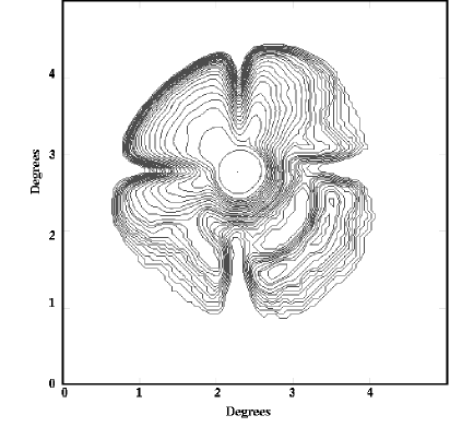
Figure 4: Sensitivity map of one of the extraction regions. The 30 contours are logarithmically spaced in sensitivity from $3.9\times 10^{-1}$ to $2.2\times 10^{-4}$.

3.2 Sensitivity maps and conversion factors

In order to build up sensitivity maps (i.e. the functions $f(\vec{x}_{b},\vec{x})$ for each of the 16 values of $\vec{x}_{b}$) we have carried out simulations, using a ray-tracing routine, to study the properties of the X-ray telescope (XRT) that focuses the X-rays. The details of the ray-tracing code can be found in Kunieda, Furuzawa & Watanabe (1995) and Gendreau & Yaqoob (1997). Basically it takes every photon, whose energy and incidence angle are known, and does a Monte Carlo simulation of its possible trajectories, including reflection in the telescope mirrors, absorption, multiple scatterings etc… The parameters governing the various processes have been updated after experience has been accumulated on the behaviour of the XRT.

In order to construct the sensitivity map for each extraction region, a uniform distribution of sources has been simulated in a $4^{\circ}\times 4^{\circ}$ region around the optical axis. Each source was assigned a flux according to a $N(S)$ (although this is irrelevant for this specific purpose). The number of photons coming from each source was computed assuming a geometric area of $882{\rm cm}^{2}$ for the XRT and a source spectrum with an energy spectral index of $0.7$. That produced a list of photons with their corresponding energies and incident positions in the sky. These photon lists were then ray-traced using the above code.

Since each photon carried labels with its original incoming direction, it was possible to build a sensitivity map. The incoming positions in the sky of the photons collected in each one of the particular extraction boxes were recorded. The density of these positions in the sky, properly normalized, is the sensitivity function.

Fig. 4 shows a contour diagram with the sensitivity map of one of the 16 extraction regions. In that map it can be seen that there is sensitivity out to very large offset angles. In the same figure it can also be noted that the sensitivity map has strong gradients, particularly close to the “cross”. (This shape results from the quadrant construction of the telescope).

Figure 5: The top curve shows the distribution in $\log f$, $f$ being the sensitivity in one of the extraction regions, obtained from the ray-tracing simulations. The two bottom curves show the same distribution but for a fixed constant value of the intensity produced by a single source, assuming a single power-law model for the source counts (see text for details). A horizontal line would represent equal contribution from each decade in sensitivity.

To emphasize the effect of the extent of the sensitivity functions, Fig. 5 shows the distribution function for the sensitivities in a specific spatial bin $f$ when smoothed on 1 arcmin² bins. The contribution to the total intensity received in a given spatial bin by sources in different directions is weighted by this distribution (top line in Fig. 5). Indeed, for a uniform distribution of sources $P(\log f)$ measures the relative contribution to this total intensity from different values of $\log f$. Fig. 5 emphasizes that the contribution from markedly off-axis sources ($f\sim 10^{-3}$) is at least as important as the one from the on-axis sources ($f\sim 1$) when computing the total intensity. Therefore stray light has to be accurately modelled if an absolute measurement of the XRB intensity needs to be done.

To study whether the XRB fluctuations are also dominated by off-axis sources, we recall that these fluctuations will be dominated by a very limited range of intensities, corresponding to the dispersion in the distribution of the fluctuations. We then construct the bivariate distribution of intensity $I$ and sensitivity $\log f$ for a given spatial bin. The intensity produced by a single source with flux $S$ in a particular bin is $I=f\,S$. Using a single power-law form for the differential source counts with slope $\gamma$ the bivariate function for $I$ and $\log f$ is

$$P(\log f;I)\propto I^{-\gamma}f^{\gamma-1}P(\log f)$$ (8)

Fig. 5 also shows this distribution for constant $I$ and different values for $\gamma$ (lower curves) for an arbitrary constant value of the intensity $I$. Therefore, the contribution to the XRB fluctuations (which are dominated by a specific value of $I$) from sources at different positions in the sky (i.e., different sensitivities) is measured by this bivariate distribution for constant $I$. Fig. 5 emphasizes that for any reasonable slope of the source counts, the fluctuations will always be dominated by sources within the nominal field-of-view of the corresponding spatial bin ($f\sim 1$). Therefore, stray light does not dominate the XRB fluctuations in this case, although it is very important for the computation of the average intensity received in each spatial bin.

In order to perform the integration of eq (6), the sensitivity functions have been computed with 1 arcmin² resolution (as in Fig. 5) which represents a compromise between good statistics in the extended low sensitivity tails and smoothing the regions with strong gradients.

With the ray-tracing simulations we also computed the conversion factors introduced in eq. (2). A bright source was placed in the middle of each bin, its photons were ray traced and only those which landed on the bin itself were counted. A detector efficiency model was used (Gendreau 1995) to convert from photons to counts (i.e., the function $F_{2}(\vec{x}_{b})$. The RDD effects discussed in section 2 were incorporated into that detector efficiency model both to estimate the conversion factor $C(\vec{x}_{b})$ and the non-X-ray detector background $I_{det}(\vec{x}_{b})$.

4 Results

4.1 The fitting process

Given that each one of the 16 extraction regions has a different sensitivity function and a different conversion factor, and that RDD changes the conversion factor for each observation, a model for the XRB fluctuations had to be computed for each one of the 240 data points, for every set of values of parameter space. For every set of values in parameter space a model distribution (eqs. 5-7) was computed for each one of the measured intensities, taking into account the different sensitivity functions (this is different for each one of the 16 extraction regions), the different conversion factors (for a given extraction region it also changes from image to image due to the RDD) and different exposure times. Particular attention was paid to the fact that the mean intensity expected for each data point is not known with infinite accuracy, due to the statistical uncertainty in the measurement of the cosmic XRB, and also possible overall inaccuracies in the conversion factors or sensitivity functions. This is why we prefer to fit the mean value of the intensity rather than impose it. The mean expected value for a given data point is

$$\langle I(\vec{x}_{b})\rangle=C(\vec{x}_{b})\Omega(\vec{x}_{b})\int_{S_{min}}^{S_{max}}dS\,N(S)+I_{det}(\vec{x}_{b})$$ (9)

where

$$\Omega(\vec{x}_{b})=\int d^{2}x\,f(\vec{x}_{b},\vec{x})$$ (10)

is the effective solid angle for flux collection. Here we take $S_{min}=3\times 10^{-11}\,{\rm erg}\,{\rm cm}^{-2}\,{\rm s}^{-1}$ (which is the completeness limit of the Piccinotti et al sample, and whose sources were certainly not near the ASCA images) and $S_{min}$ is either the flux at which the XRB saturates or $10^{-15}\,{\rm erg}\,{\rm cm}^{-2}\,{\rm s}^{-1}$ (small enough so that fluctuations produced by fainter fluxes will be absolutely negligible) when the slope of the source counts is too flat to saturate the XRB. Then, the quantity

$$X={I(\vec{x}_{b})-I_{det}(\vec{x}_{b})\over C(\vec{x}_{b})\Omega(\vec{x}_{b})}$$ (11)

should not depend on extraction box or detector efficiency and reflect only sky fluctuations and counting noise. We evaluated the average of this quantity $\langle X\rangle_{obs}$ and its uncertainty $\sigma(\langle X\rangle)_{obs}$ using the 240 data points themselves. In the fitting process, however, $\langle X\rangle$ was a free parameter and was fitted (and considered non-interesting) but adding the following contribution to the $\chi^{2}$ to reflect our knowledge on its value, i.e.

$$\left({\langle X\rangle-\langle X\rangle_{obs}\over\sigma(\langle X\rangle)_{obs}}\right)^{2}.$$ (12)

A number of tests were performed to check on the accuracy of our fitting method (and model) by generating simulated images with model source counts and then analyzing them with the same procedure that was later applied to the data. Both a maximum likelihood method and a $\chi^{2}$ method (where the intensity histogram was binned in groups of at least 15 data points to ensure proper statistics) were tried. As a general result, the maximum likelihood method almost invariably found much higher source counts than the input ones, especially when bright sources were present. The $\chi^{2}$ minimisation proved rather accurate in defining the value of the source counts in the range of fluxes where this analysis is sensitive ($\sim(2-13)\times 10^{-14}{\rm erg}\,{\rm cm}^{-2}\,{\rm s}^{-1}$ for the real data), although the shape of the source counts within this flux range is very poorly constrained by a sample of this size and depth.

4.2 Single power law source count models

We assume that the source counts follow a power-law distribution

$$N(S)={K\over S_{0}}(\gamma-1)\left({S\over S_{0}}\right)^{-\gamma}$$ (13)

where the reference flux $S_{0}$ is chosen at $10^{-13}{\rm erg}\,{\rm cm}^{-2}\,{\rm s}^{-1}$ (which is close to the flux where the fluctuation analysis is most sensitive) and $K$ is the number of sources per solid angle brighter than $S_{0}$. Results from GINGA fluctuation analyses (Butcher et al 1997) predict values of $K=400\,\deg^{-2}$ and $\gamma\approx 2.5$, if they can be extrapolated to these lower fluxes. On the contrary, if a conversion from the ROSAT source counts in the 0.5-2 keV band to our 2-10 keV band in terms of a single power law X-ray spectrum with energy spectral index of $0.7$ is assumed, then a normalisation closer to $K=150\,\deg^{-2}$ would apply.

Figure 6: Best fit and confidence regions for 1, 2 and 3 $\sigma$ for a single power law model. The dotted line shows those points which will be consistent with the HEAO-1 A2 point of Piccinotti et al (1982).

Figure 7: The 2-10 keV integral source counts. The data points are from: A2 by Piccinotti et al (1982), LSS by Ueda (1995), DSS by Inoue et al (1996), G97 by Georgantopoulos et al (1997). The ‘trumpet’ is the 1$\sigma$ region delimited by our analysis. The dashed line shows the saturation level for the XRB assuming $\gamma=2.5$.

The results from the fitting process are shown in Fig. 6 in ($K$,$\gamma$) space. The best fit corresponds to $K\approx 200\,\deg^{-2}$ and $\gamma\approx 2.3$ with a $\chi^{2}=17.33$ for 13 degrees of freedom (16 bins minus 3 fitted parameters) resulting in a fairly small reduced $\chi^{2}/N_{\rm dof}\sim 1.3$. There is, however, no obvious systematic difference between the histogrammed data and the best-fit model (see again Fig. 3).

In Fig. 6 it can also be seen that there is a degeneracy between values of $K$ and $\gamma$ which are very poorly constrained individually. When $K$ is considered the only interesting parameter, it can take any value from 100 to 750 $\deg^{-2}$ (1$\sigma$ interval). A similar analysis for $\gamma$ yields a 1$\sigma$ interval that ranges from $\gamma\sim 2$ to $\gamma\sim 3$.

However, if the source counts are forced to have an euclidean shape, then the normalisation is fairly well constrained to $K=(300\pm 100)\,\deg^{-2}$ (1$\sigma$ errors), the ROSAT normalisation $K=150\,\deg^{-2}$ being only 2$\sigma$ below in this case.

In spite of the fact that the parameters $K$ and $\gamma$ are poorly constrained individually, as expected from the simulations the source counts in the region between $(2-12)\times 10^{-14}{\rm erg}\,{\rm cm}^{-2}\,{\rm s}^{-1}$ are fairly well constrained by our analysis. Fig. 7 shows this result in terms of the integral source counts together with the results of the various surveys (errors are 1$\sigma$ always). Our result is consistent with the ASCA LSS (Ueda 1995) and the ASCA DSS (Inoue et al 1996), but the Georgantopoulos et al (1997) source counts down to $5\times 10^{-14}{\rm erg}\,{\rm cm}^{-2}\,{\rm s}^{-1}$ are significantly higher than what we find in our analysis. In fact they are about 3$\sigma$ above from our result. The reasons for this discrepancy (and also the disagreement between Georgantopoulos et al 1997 and the ASCA DSS) are unclear, but small number statistics, source variability, confusion and Eddington bias are among the possibilities. In particular, as recognised by Georgantopoulos et al (1997), Eddington bias and confusion could well produce errors of the order of 100 per cent in the fluxes of the faintest sources.

A slight modification applies to our source counts if the source spectra are flatter. If an energy spectral index of $0.4$ (similar to that of the XRB) is assumed instead of the canonical $0.7$, larger fluxes are needed to produce the same intensities due to the dominant response of the XRT+SIS0 at low energies. In this case, our estimates of the source counts shown in Fig. 7 would have to be displaced to higher fluxes by rougly 15 per cent which is the average ratio between conversion factors (as defined in eq. 2) for energy spectral indices 0.4 to 0.7. For the approximately euclidean source counts, this means that our source counts will go up by $\sim 25$ per cent, still significantly lower than the Georgantopoulos et al (1997) source counts.

4.3 Broken power law source counts

As discussed earlier, soft X-ray source counts found by ROSAT exhibit a break from an approximately euclidean slope above a 0.5-2 keV flux of $2\times 10^{-14}{\rm erg}\,{\rm cm}^{-2}\,{\rm s}^{-1}$. Converting that break flux into the 2-10 keV band requires detailed knowledge of the broad-band average X-ray spectrum of the sources at that flux, which is not known. Alternatively, if a break in the 2-10 keV source counts is found and is identified with the ROSAT one, an approximate conversion factor between the 0.5-2 and 2-10 keV bands could be found.

Therefore, we tested also a broken-power law source counts model, which fits the 2-10 keV source counts at bright fluxes (i.e., eq.(13) with $K=400\,\deg^{-2}$ and $\gamma=2.5$) down to a break flux $S_{b}$ below which the source counts flatten to a slope $\gamma$. After modelling the source counts in terms of these two free parameters, it was found that all values of $S_{b}$ were within 1$\sigma$ of the best fit for $\gamma<2.5$ and $S_{b}>3\times 10^{-14}{\rm erg}\,{\rm cm}^{-2}\,{\rm s}^{-1}$.

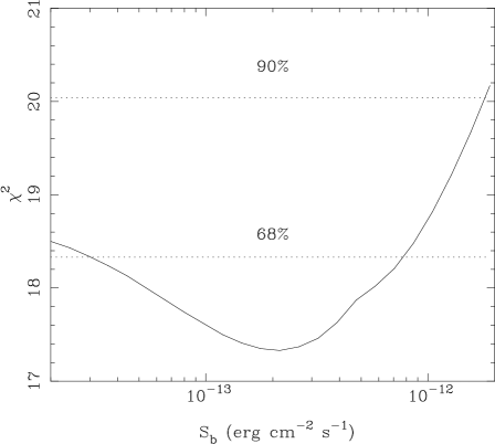
Figure 8: $\chi^{2}$ for the break flux $S_{b}$ in a broken power law model where the slope below $S_{b}$ has been taken $\gamma=1.8$.

A further test was carried out, by fixing the slope below the break to the value found by ROSAT ($\gamma=1.8$). $\chi^{2}$ as a function of the break flux $S_{b}$ is plotted in Fig. 8. The best fit is $\log(S_{b})=-12.7^{+0.5}_{-0.8}$ (1$\sigma$). The 90 per cent confidence upper limit is $\log(S_{b})<-11.7$. Unfortunately these limits do not impose any relevant constraints on the broad band spectrum of the sources, which is only restricted to have an energy spectral index of less than 0.9 ($1\sigma$).

5 Discussion and future work

In this paper we have found that the extrapolation of euclidean power-law source counts from higher fluxes appears to be consistent with the fluctuations in deep ASCA SIS0 images down to a flux of $\sim 2\times 10^{-14}{\rm erg}\,{\rm cm}^{-2}\,{\rm s}^{-1}$. Adopting the euclidean form, there must be $(300\pm 100)\,\deg^{-2}$ sources brighter than a 2-10 keV flux of $10^{-14}{\rm erg}\,{\rm cm}^{-2}\,{\rm s}^{-1}$. Down to the flux where our fluctuation analysis is sensitive ($2\times 10^{-14}{\rm erg}\,{\rm cm}^{-2}\,{\rm s}^{-1}$) the integrated intensity of the sources represents $35\pm 13$ per cent of the XRB as measured by the ASCA SIS (Gendreau et al 1995). There is no evidence for a break in the source counts although it cannot be excluded. For reasonable source spectra, the break that is seen in soft X-ray source counts is expected to occur around the faintest flux at which the fluctuation analysis is sensitive, so it is difficult to detect.

Although the analysis of the fluctuations in a telescope which has such an extended sensitivity is complicated, we have shown that the analysis can be done if all effects are properly modelled. The major limitation in our results comes from the limited field of view of the SIS0 detector. The next step would be to use GIS images of the same fields to increase by a factor of several the solid angle surveyed and, hopefully, reduce the uncertainties in the determination of the source counts by a factor of at least 2.

Another issue that can be addressed with the fluctuation analyses is that of the average spectrum of the sources. Given the fairly good spectral resolution of both the SIS and the GIS, fluctuations in two different energy bands can be fitted to the same source counts, the major unknown being the spectral shape linking both bands. Modelling the spectrum in terms of a single power law, will allow the average energy spectral index of the sources in the flux range $(2-12)\times 10^{-14}{\rm erg}\,{\rm cm}^{-2}\,{\rm s}^{-1}$ being determined. That particular approach proved useful in deriving the soft X-ray spectrum of very faint sources by analysing the fluctuations in ROSAT PSPC deep images (Ceballos, Barcons & Carrera 1997).

References

- [1] Almaini, O., Shanks, T., Boyle, B.J., Griffiths, R.E., Roche, N., Stewart, G.C., Georgantopoulos, I., 1996, MNRAS, 282, 295
- [2] Barcons, X., Fabian, A.C., 1990, MNRAS, 243, 366
- [3] Barcons, X., Branduardi-Raymont, G., Warwick, R.S., Mason, K.O., McHardy, I.M., Rowan-Robinson, M., 1994, MNRAS, 268, 833
- [4] Barcons, X., Fabian, A.C., Carrera, F.J., 1997, MNRAS, in the press (astro-ph/9705180)
- [5] Branduardi-Raymont, G. et al 1994, MNRAS, 270, 947
- [6] Butcher, J.A., Stewart, G.C., Warwick, R.S., Fabian, A.C., Carrera, F.J., Barcons, X., Hayashida, K., Inoue, H., Kii, T., 1997, MNRAS, in the press (astro-ph/9707135)
- [7] Ceballos, M.T., Barcons, X., Carrera, F.J., 1997, MNRAS, 286, 158
- [8] Condon, J.J., 1974, ApJ, 188, 279
- [9] Dotani, T., Yamashita, A., Rasmussen, A., 1995, ASCA News, 3, 25
- [10] Fabian, A.C., Barcons, X., 1992, ARA&A, 30, 429
- [11] Gendreau, K.C., 1995, PASJ, 47, L5
- [12] Gendreau, K.C., Yaqoob, T., 1997, ASCA News 5, 8
- [13] Gendreau, K.C., 1995, Ph.D. Thesis, MIT
- [14] Georgantopoulos, I., Stewart, G.C., Blair, A.J., Shanks, T., Griffiths, R.E., Boyle, B.J., Almaini, O., Roche, N., MNRAS, in the press (astro-ph/9704147)
- [15] Hamilton, T.T., Helfand, D.J., 1987, ApJ, 318, 93
- [16] Hasinger, G., Burg, R., Giacconi, R., Hartner, G., Schmidt, M., Trümper, J., Zamorani, G., 1993, A&A, 175, 1
- [17] Hasinger G., Burg R., Giacconi R., Schmidt M., Trümper J., Zamorani G., 1997, A&A, in the press (astro-ph/9709142)
- [18] Hayashida, K., 1989, Ph.D. Thesis, University of Kyoto
- [19] Inoue, H., Kii, T., Ogasaka, Y., Takahashi, T., Ueda, Y., 1996, MPE Report, 263, 323
- [20] Kondo, H., 1991, Ph.D. Thesis, University of Tokyo
- [21] Kunieda, H., Furuzawa, A., Watanabe, M., 1995, ASCA News, 3, 3
- [22] McHardy, I.M., et al 1997, MNRAS, in the press (astro-ph/9703163)
- [23] Piccinotti, G., Mushotzky, R.F., Boldt, E.A., Holt, S.S., Marshall, F.E., Serlemitsos, P.J., Shafer, R.A., 1982, ApJ, 253, 485
- [24] Romero-Colmenero, E., Branduardi-Raymont, G., Carrera, F.J., Jones, L.R., Mason, K.O., McHardy, I.M., Mittaz, J.P.D., 1996, MNRAS, 282, 94
- [25] Scheuer, P.A.G., 1974, MNRAS, 166, 329
- [26] Schmidt M. et al, 1997, A&A, in the press (astro-ph/9709144)
- [27] Tanaka, Y., Inoue, H., Holt, S.S., 1994, PASJ, 46, L37
- [28] Ueda, Y., 1995, Ph. D. Thesis, University of Tokyo