Detection of Magnetic Fields Toward M17 through the
H i Zeeman Effect

Abstract

We have carried out VLA Zeeman observations of H i absorption lines toward the H ii region in the M17 giant molecular cloud complex. The resulting maps have 60$\times$45 spatial resolution and 0.64 km s^-1 velocity separation. The H i absorption lines toward M17 show between 5 and 8 distinct velocity components which vary spatially in a complex manner across the source. We explore possible physical connections between these components and the M17 region based on calculations of H i column densities, line of sight magnetic field strengths, as well as comparisons with a wide array of previous optical, infrared, and radio observations.

In particular, an H i component at the same velocity as the southwestern molecular cloud (M17 SW) $\sim 20$ km s^-1 seems to originate from the edge-on interface between the H ii region and M17 SW, in un-shocked PDR gas. We have detected a steep enhancement in the 20 km s^-1 H i column density and line of sight magnetic field strengths ($B_{los}$) toward this boundary. A lower limit for the peak 20 km s^-1 H i column density is $N_{HI}$/$T_{s}\geq 5.6~{}\times 10^{19}$ cm^-2/K while the peak $B_{los}$ is $\sim-$450 $\mu$G. In addition, blended components at velocities of 11$-$17 km s^-1 appear to originate from shocked gas in the PDR between the H ii region and an extension of M17 SW, which partially obscures the southern bar of the H ii region. The peak $N_{HI}$/$T_{s}$ and $B_{los}$ for this component are $\geq 4.4\times 10^{19}$ cm^-2/K and $\sim+550$ $\mu$G, respectively. Comparison of the peak magnetic fields detected toward M17 with virial equilibrium calculations suggest that $\approx 1/3$ of M17 SW’s total support comes from its static magnetic field and the other 2/3 from its turbulent kinetic energy which includes support from Alfvén waves.

Brogan et al. Magnetic Fields Toward M17

and brogan@pa.uky.edu

1 INTRODUCTION

In recent years it has become increasingly clear that magnetic fields play an important role in the process of star formation. (See, for example,mou76 Mouschovias & Spitzer 1976; heiHeiles et al. 1993;mck93 Mckee et al. 1993). Unfortunately, the experimental techniques for measuring the strength and direction of magnetic fields are few and these methods are observationally challenging. One such technique uses the Zeeman effect in 21 cm H i absorption lines toward galactic H ii regions. Very Large Array (VLA) observations of the Zeeman effect in this line yield maps of the line-of-sight magnetic field strengths ($B_{los}$). These maps can then be compared to maps of the distribution and kinematics of ionized, atomic, and molecular gas to study the role of magnetic fields in star forming regions. Moreover, estimates of the masses, column densities, and volume densities of interstellar material associated with the star-forming regions can be compared to field strengths measured via the Zeeman effect. These comparisons are needed to determine the energetic importance of magnetic fields in star-forming regions. For studies of this type, the M17 H ii region$-$molecular cloud complex is ideal because it has been extensively studied at many wavelengths.

The M17 H ii region is one of the strongest thermal radio sources in our galaxy. Its distance has been estimated through photometric and kinematic means to be $\sim$ 2.2 kpc (Chini, Elsässer, & Neckel chin 1980;reif Reifenstein et al. 1970;wil Wilson et al. 1970). There are at least 100 stars in the M17 H ii region with one O4 V (Kleinmann’s star) and three O5 V stars providing the bulk of the ionizing radiation (felFelli, Churchwell, & Massi 1984 and references therein; see Fig. 1). The H ii region is made up of two distinct bar like structures which are $\sim 5.7$ pc long and $\sim 1.1$ to 1.5 pc wide. The southern bar has nearly twice the peak radio continuum flux as the northern bar, and is located just to the east of the M17 SW molecular cloud core.

The near absence of optical radiation from the southern bar indicates that this region suffers much more optical extinction than the northern bar (gulGull & Balick 1974, Fig 1). dicDickel (1968) and gatGately et al. (1979) estimate $A_{v}\sim$ 1-2 mag toward the northern bar. Estimates of the visual extinction toward the southern bar range from $A_{v}\sim 10$ near the radio continuum peak to $A_{v}\sim 200$ further west toward the core of the adjacent molecular cloud (M17 SW) (beetzBeetz et al. 1976; felFelli et al. 1984; gatGatley et al. 1979; throThronson & Lada 1983). The low extinction toward the northern bar seems to indicate that the northern molecular cloud, first identified by lad76Lada et al. (1976) ($v_{LSR}\sim 23$ km s^-1), is behind the H ii region (chrysChrysostomou et al. 1992).

The most interesting characteristic of M17 is that the interface between the southern bar of the H ii region and M17 SW is seen almost edge on (Fig. 1). From models of the density gradient on the western edge of the H ii region, ickIcke, Gatley, & Israel (1980) estimated that this interface lies at an angle of $\sim 20\arcdeg$ with respect to the line of sight. Although the transition from the H ii region to the molecular cloud is quite sharp, the interface region is too wide in photodissociation region (PDR) tracers such as [C ii] 158 $\mu$m unless it is clumpy (see eg., stut88Stutzki et al. 1988). The extended [C ii] 158 $\mu$m emission observed in M17 SW by stut88Stutzki et al. (1988) and borBoreiko, Betz, & Zmuidzinas (1990) requires 912-2000Å UV photons to persist into the molecular cloud at least an order of magnitude further than the predicted UV absorption length scale. That is, atoms are being photoionized and molecules photodissociated further into the molecular cloud than one would expect for a homogeneous medium. (See teiTielens & Hollenbach 1985 for homogeneous model calculations.) A possible explanation for this paradox is that the interface region is clumpy.

Evidence that M17 SW is clumpy has been observed with high angular resolution at many

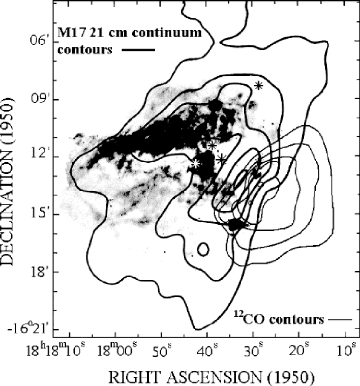
Figure 1: Map of the 1, 5, 10, 20, and 30 Jy beam^-1 21 cm continuum contours (present work, (thick lines) superimposed on an optical image from Gull & Balick and simplified ¹²CO contours (thin lines) from Thronson & Lada (1983). The four stars which are primarily responsible for ionizing the H ii region are indicated with star symbols, with the largest representing Kleinmann’s star (Felli, Churchwell, & Massi 1984) .

wavelengths. For example, felFelli et al. (1984), found clumpiness in their $\sim 10\arcsec$ resolution radio continuum observations of the M17 H ii region. They suggest this clumpiness originates from high density neutral clumps surrounded by dense ionized envelopes. These clumps may be the remnants of clumps from the parent molecular cloud which have been overtaken by the H ii region ionization front. masMassi, Churchwell, & Felli (1988) observed seven clumps in NH₃ emission with 6 resolution toward the northwestern portion of the H ii region$-$M17 SW interface. The average density and size of these clumps are $n_{H_{2}}\sim 10^{7}$ cm^-3 and 0.05 pc. stut90Stutzki & Güsten (1990) modeled their $\sim 13\arcsec$ resolution C¹⁸O ($2\rightarrow 1$) observation (with a larger field of view than the NH₃ observation) with $\sim 180$ clumps with average densities of $n_{H_{2}}$ $\sim 10^{5-6}$ cm^-3 and diameters of $\sim$ 0.1 pc. hob92Hobson (1992) also saw evidence for clumpiness in HCO⁺ and HCN molecules at $\sim 19\arcsec$ resolution, and wanWang et al. (1993) found clumps consistent with the C¹⁸O clumps in $\sim 18\arcsec$ to $\sim 34\arcsec$ resolution observations of CS and C³⁴S molecules.

The identification of clumps in M17 SW is significant for several reasons. For example, calculations of density are more complex due to its dependence on the optical depth of the observed species, and the assumed clump filling factor. As discussed previously, the lengthscale of the PDR also depends on the clumpiness of the region. Therefore, the regions and morphology of photodissociated atomic gas are difficult to predict. Also the random motion of such clumps can influence observed linewidths and the sizescale of turbulence within the molecular cloud. These considerations play an important role in our analysis of the H i gas and the line of sight magnetic fields calculated from it.

In this paper we report the characteristics of the 21 cm continuum (§3.1), H i optical depths and column densities (§3.2), and the line of sight magnetic field strengths (§3.3) derived from our VLA H i Zeeman effect observation. We discuss possible origins for the most prominent H i absorption components in §4.1. In addition, we present comparisons of our 20 km s^-1 $B_{los}$ map with previous linear polarimetry observations in §4.2, and we also compare expected magnetic field strengths from virial equilibrium arguments to our observed line of sight magnetic field strengths in §4.3. Our findings are summarized in §5.

2 OBSERVATIONS

tab1

Our H i absorption data were obtained with the DnC configuration of the VLA . Key parameters from this observation can be found in Table 1. We observed both senses of circular polarization simultaneously. Since the Zeeman effect is very sensitive to small variations in the bandpass, we switched the sense of circular polarization passing through each telescope’s IF system every 10 minutes with a front-end transfer switch. In addition, we observed each of the calibration sources at frequencies shifted by $\pm$ 1.2 MHz from the H i rest frequency to avoid contamination from Galactic H i emission at velocities near those of M17.

The calibration, map making, cleaning, and calculation of optical depths were all carried out using the AIPS (Astronomical Image Processing System) package of the NRAO. The right (RCP) and left (LCP) circular polarization data were separately calibrated and mapped using natural weighting. These two data cubes were then combined to create Stokes I (RCP + LCP) and Stokes V (RCP $-$ LCP) cubes. The I and V cubes were CLEANed using the AIPS task SDCLN down to 70 mJy beam^-1. Bandpass correction was applied only to the I data since bandpass effects subtract out to first order in the V data. Subsequent antenna leakage correction and magnetic field derivations were carried out using the MIRIAD (Multichannel Image Reconstruction Image Analysis and Display) processing package from BIMA.

3 RESULTS

3.1 The 21 cm Continuum

figu1

Figure 1 shows our 21 cm continuum contours with an optical image from Gull & Balick gul (1974) and simplified ¹²CO contours from throThronson & Lada (1983) superimposed. The total continuum flux at 21 cm is $\sim 800$ Jy calculated inside the 1 Jy beam^-1 (250 K) contour level (lowest contour in Fig. 1). This value is almost twice that obtained by Lockhart & Goss loc (1978) with a 2 beam at the Owens Valley interferometer. In addition, we estimate the total flux of the Southern bar is 384 Jy while that of the Northern bar is 240 Jy (calculated for points inside the 5 Jy beam^-1 contour level). Our total flux inside the 5 Jy beam^-1 contour (624 Jy) is similar to the 644 Jy reported by Lada et al. lad76 (1976) with the Haystack 120 ft telescope and 620 Jy observed by Löbert & Goss lob (1978) with the Fleurs synthesis telescope at 21 cm.

3.2 Atomic Hydrogen Optical Depths and Column Densities

figu2

M17 H i optical depths were calculated assuming that the spin temperature $T_{s}$ is much less than the background continuum temperature $T_{c}$ of the H ii region. In addition, optical depth calculations were restricted to positions where the continuum power is greater than 1 Jy beam^-1 (250 K) and the signal-to-noise ratio is higher than three. The complex nature of the absorption lines in M17 can be seen from the optical depth spectra displayed in Figure 2. The strengths of some components vary spatially over the source but remain distinct, while other components seem limited to particular regions. This complexity makes Gaussian fitting very difficult. Our profiles agree qualitatively with the Gaussian fits reported by loc Lockhart & Goss (1978) made with a $2\arcmin$ beam and 0.85 km s^-1 velocity resolution. They fit their M17 H i optical depth profiles with eight Gaussians having center velocities ranging from 4.2 to 27.5 km s^-1. In the following analysis we concentrate on the H i velocity component near 20 km s^-1 and the blended components between 11$-$17 km s^-1 due to their high optical depths and their coincidence in velocity with other species observed in M17 SW (see §4.1 for details).

figu3

Figure 3 displays the morphology of the H i optical depths toward the M17 H ii region as a function of velocity (every two adjacent channels were averaged). The steep increase of the H i optical depth toward the H ii region$-$molecular cloud interface is clearly apparent. This effect is particularly noticeable near 20 km s^-1. Although the H i optical depths become saturated at the western boundary of the H ii region (particularly in the northwest), they reach values at least as high as 5. Optical depth maps in the 11$-$17 km s^-1 range have their highest values further to the east and in the northern part of the source.

figu4

The column density of H i toward M17 was found using the relationship

$$N_{HI}=1.823\times 10^{18}T_{s}\int\tau_{\nu}d\nu~{}{\rm cm^{-2}},$$ (1)

where $\tau_{\nu}$ is the optical depth per unit frequency. Values for $N_{HI}$/$T_{s}$ summed across the entire H i velocity range, the 20 km s^-1 component (from 17 to 24.5 km s^-1) and the 11$-$17 km s^-1 blended component are displayed in Figs. 4a, 4b, and 4c, respectively. At positions along the northwest and southwest portions of the source, these maps represent lower limits to $N_{HI}$/$T_{s}$ owing to saturation effects. Note the increase in the H i column density toward the H ii region$-$molecular cloud interface on the southwestern side of the maps. There is also spatial agreement between the H i column density concentration prominent in the total $N_{HI}$/$T_{s}$ map (Fig. 4a) near $18{\rm{}^{h}}17{\rm{}^{m}}30.0{\rm{}^{s}}$, ${-16}\arcdeg 13\arcmin 05\arcsec$ and the northern condensation seen

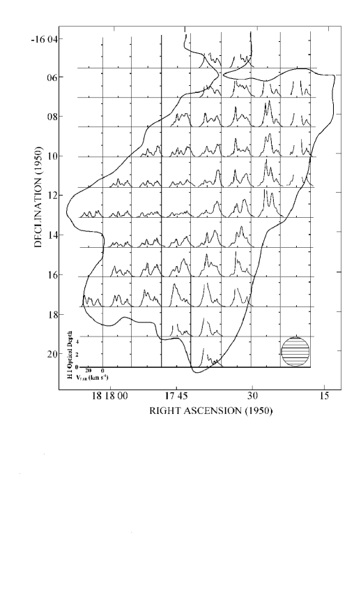
[cryopt15.eps]H i Optical depth profiles across the source after convolution with a 2 beam (each profile is independent). The 1 Jy beam^-1 21 cm continuum contour, and $2\arcmin$ beam are shown for reference .                  

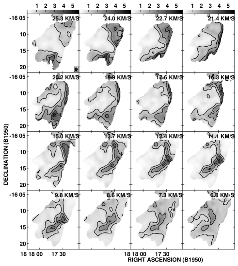
Figure 2: Velocity channel maps of the H i optical depth morphology (after averaging every two channels) from 6.0 to 25.3 km s^-1 (greyscale), with contours at $\tau=$1, 2, 3, 4, and 5. Notice the increase in H i optical depths as you approach M17 SW in the 24.0 to 17.6 km s^-1 velocity range .

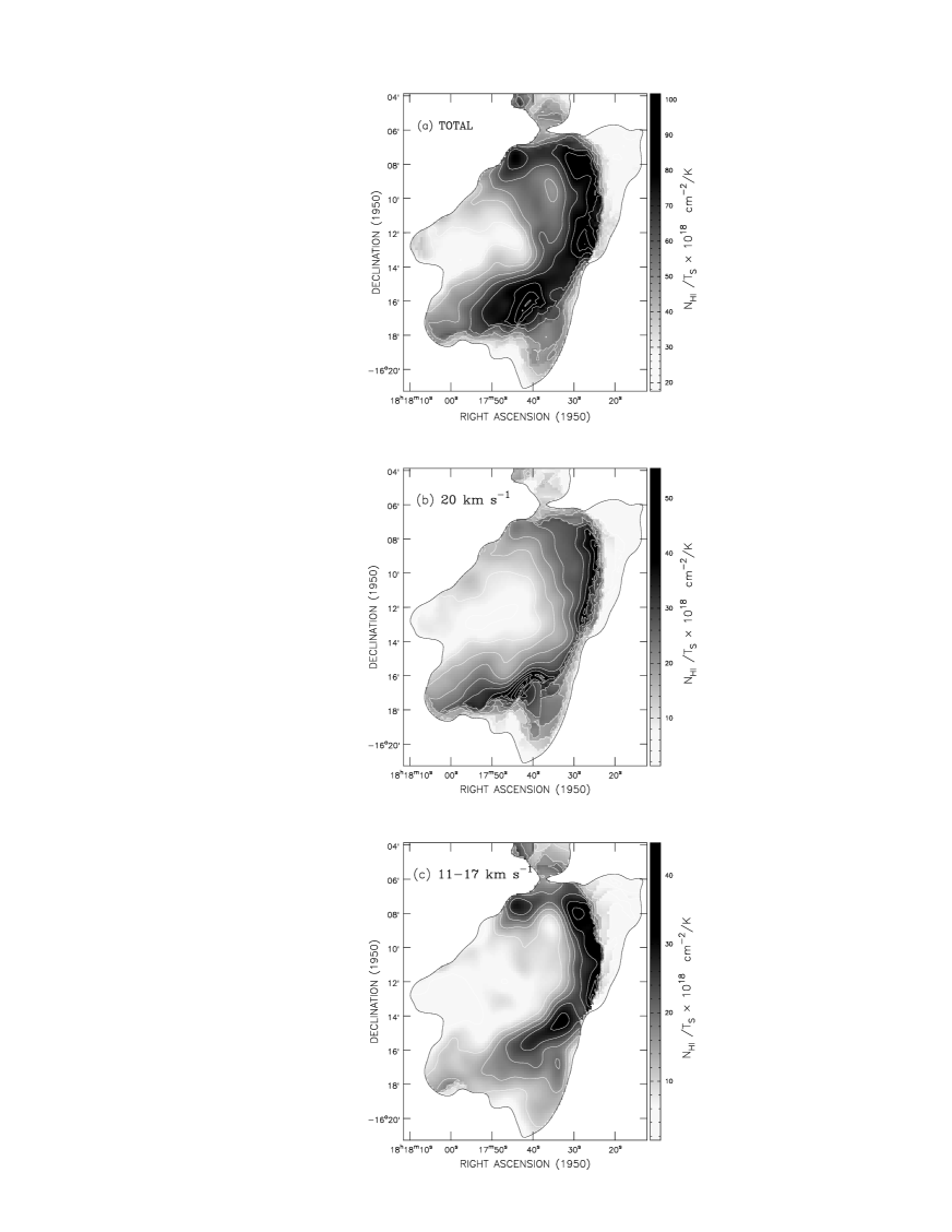
Figure 3: Maps of H i column density divided by spin temperature ($N_{HI}/T_{s}$) calculated using equation (1). For each map the outermost black contour is the 1 Jy beam^-1 21 cm continuum level, and the greyscale and white contours represent $N_{HI}/T_{s}\times 10^{18}$ cm^-2/K. (a) Data summed across the $entire$ H i line. White contour levels are in increments of $10\times 10^{18}$ cm^-2/K from 20 to 100 $\times 10^{18}$ cm^-2/K, (b) Data for the 20 km s^-1 component summed from 17 to 24.5 km s^-1. White contour levels are in increments of 5 $\times 10^{18}$ cm^-2/K from 5 to 55 $\times 10^{18}$ cm^-2/K, and (c) Data for the 11 to 17 km s^-1 component summed from 10.5 to 16.9 km s^-1. White contour levels are in increments of 5 $\times 10^{18}$ cm^-2/K from 5 to 40 $\times 10^{18}$ cm^-2/K .

in molecular gas (see wan Wang et al. 1993 and Fig. 8). The total $N_{HI}/T_{s}$ at this position is 8.3 $\times 10^{19}$ cm^-2/K.

Aside from line saturation, the main source of uncertainty in calculating H i column densities is in the value assumed for $T_{s}$. Upper limits to $T_{s}$ come from two sources. For one, the H i line widths in some cases are quite narrow. Toward the southern end of the molecular ridge defined by CS emission (wanWang et al. 1993) they are as little as 2.8 km s^-1 for the 20 km s^-1 component (Figs. 8, 9). This width implies a maximum temperature of 180 K at this position. Also, along the periphery of the continuum source, H i absorption lines exist where the continuum brightness is as little as 250 K (1 Jy beam^-1). Evidently, $T_{s}$ is less than about 200 K in many directions toward M17. At the position illustrated in Fig. 9, the CS line has a width of about 2 km s^-1. If H i and CS are mixed and at a common temperature, then $T_{s}\approx$100 K. In fact, modeling of IRAS 12 $\mu$m infrared data byhob94Hobson & Ward-Thompson (1994) require a hot dust component of $\sim$108 K to explain the overall 12 $\mu$m emission from M17. This hot dust can be linked to the PDR by the fact that warm emission at 12 $\mu$m is likely to arise from a population of polycyclic aromatic hydrocarbons (PAHs) (desDésert, Boulanger & Puget 1990), and PAH emission from PDR regions has been predicted by many authors (e.g. holl93Hollenbach 1993).

Another indication of temperature in the atomic gas comes from the observations of [C i] 370 $\mu$m by genGenzel et al. (1988). They estimate a temperature of 50 K for [C i] 370 $\mu$m gas near 20 km s^-1. Molecular temperature determinations may also be relevant if some of the H i is mixed with molecular gas (§4.2). berginBergin et al. (1994) estimate $T_{K}$ = 50 K from observations of low-$J$ CO transitions, while harHarris et al. (1987) show that high $J$ CO lines ($7\rightarrow 6,14\rightarrow 13$) arise from PDR gas at about 250 K. meiMeixner et al. (1992) found that the spatial extent and intensities of a wide array of far-infrared and submillimeter cooling lines could be adequately modeled by a three component gas consisting of very dense clumps $n\sim 5\times 10^{5}$ cm^-3, intermediate density interclump gas $n\sim 5\times 10^{3}$ cm^-3, and a tenuous extended halo $n\sim 3\times 10^{2}$ cm^-3. They obtained the best agreement with observations by assuming an interclump gas kinetic temperature of $\sim 200$ K where it is also likely that dissociated H i gas can be found. Almost certainly, $T_{s}$ in the H i gas is quite variable, with values in the range 50 - 200 K most common.

As described above, it is likely that no one spin temperature is applicable to all of the H i gas components seen in M17. With a spin temperature of 50 K, a lower limit to the peak $total$ column density toward M17 is $N_{HI}=5.1\times 10^{21}$ cm^-2. Spin temperatures between 50 K and 200 K yield peak column densities of $2.8-11.0\times 10^{21}$ cm^-2 for the 20 km s^-1 component and $2.2-9.0\times 10^{21}$ cm^-2 for the 11$-$17 km s^-1 blended components. We can use such estimates of the H i column density to estimate what fraction of the total hydrogen column density arises from atomic gas. For example, felFelli et al. (1984) used the optical depth of the silicon absorption feature at 10 $\mu$m to estimate that $A_{\nu}$=30 toward the ultra compact H ii region M17-UC1 ($18{\rm{}^{h}}17{\rm{}^{m}}32{\rm{}^{s}},{-16}\arcdeg 13\arcmin 00\arcsec$). Using $N_{H_{TOT}}=2\times 10^{21}A_{v}$ (bert92 Bertoldi& Mckee 1992), we estimate that the total column density of hydrogen is $N_{H_{TOT}}\approx 6\times 10^{22}$ cm^-2. Our total H i column density toward M17-UC1 is $N_{HI}\geq 3.7\times 10^{21}$ cm^-2 ($T_{s}$=50 K). Unless saturation effects have resulted in a severe underestimate of $N_{HI}$, much of the gas along the line of sight to M17$-$UC1 is in the form of H₂.

3.3 Magnetic Field Strengths From the Zeeman Effect

The H i Zeeman effect is only sensitive to the line of sight magnetic field ($B_{los}$) in most astrophysical situations since the Zeeman splitting is a tiny fraction of the line width. Since V$\propto d$I$/d\nu$, values for $B_{los}$ were obtained by fitting the derivative of the I profile to the V profile at each pixel with a least squares fitting routine (for details see Roberts et al. 1993, cru96Crutcher et al. 1996). Due to the complexity of the H i spectra, the number of channels fit for each velocity component is small. To obtain more realistic error estimates, forty channels outside of the line region were included in each fit. The resulting $B_{los}$ maps were subsequently masked where the continuum power is less than 1 Jy beam^-1 and when $B_{los}$/$\sigma$($B_{los}$) $<$ 3. The quantity $B_{los}$/$\sigma$($B_{los}$) will subsequently be denoted $S/N_{B}$.

3.3.1 Magnetic Fields Derived for the 20 km s^-1 Component

figu5

Observations of M17 have been made for many astrophysically relevant molecular and atomic transitions. From these data it is known that M17 SW has a LSR velocity of 19 to 21 km s^-1 which corresponds to the velocity of one of our strongest H i absorption components. Figure 5 shows an H i optical depth profile and several molecular emission profiles from stut88Stutzki et al. (1988) for a position at the H ii region$-$molecular cloud interface. Note the similarity in the center velocities ($\sim$ 20 km s^-1) of each species. This velocity coincidence strongly suggests that the 20 km s^-1 H i absorption component is closely associated with the molecular cloud, most likely arising in the PDR at the H ii region-molecular cloud interface. Further evidence for this association comes from the steep rise in the 20 km s^-1 H i optical depth toward the interface region (Fig. 4b). Therefore, values of $B_{los}$ derived from the H i Zeeman effect in this component are of direct relevance to the energetics of the molecular cloud and its immediate surroundings (see§4.1.2).

figu6 figu7

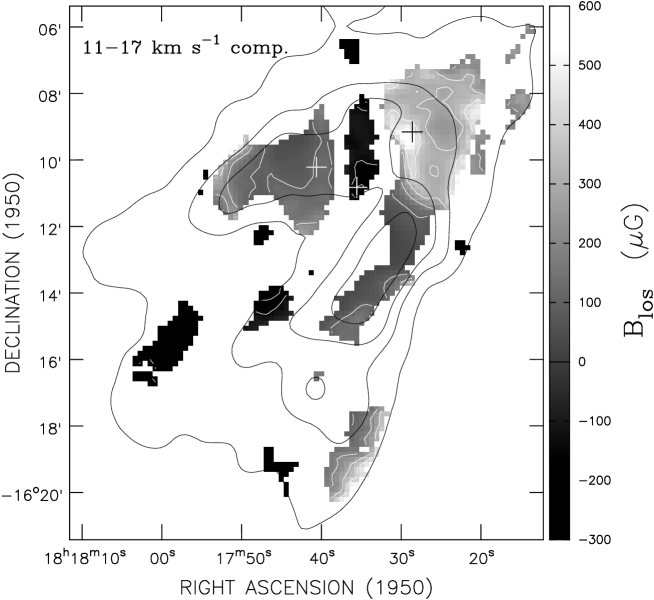
Figure 7: Greyscale map of $B_{los}$ for the 11$-$17 km s^-1 blended components with white contours at $-$250, $-$150, 100, 200, 300, 400 and 500 $\mu$G. The 21 cm continuum contours are shown in black at 1, 5, 10, and 20 Jy beam^-1. The three + symbols show the positions of the profiles shown in Fig. 11 a,b,c .

A significant magnetic field exists in the 20 km s^-1 component over much of the central region of the southern bar. The velocity range of the fit for this component is 17.0 to 24.6 km s^-1. A distinct H i component at $\sim$ 23 km s^-1 is also visible toward the northwestern corner of the source. A component at this velocity was also detected at this velocity by lad75 Lada & Chaisson (1975) in H₂CO. However, detailed inspection of the H i data cube shows that the channel range used to fit the 20 km s^-1 component was such that no magnetic field was detected in regions where the 23 km s^-1 component is distinct. Therefore, the $B_{los}$ detected in the velocity range 17 to 24.6 km s^-1 is only representative of the field in the 20 km s^-1 H i component. A map of $B_{los}$ for the 20 km s^-1 component is shown in Fig. 6, and sample fits at representative pixels are shown in Figs. 7a, 7b, and 7c. Negative values indicate that $B_{los}$ is toward the observer. Values of $B_{los}$ for this component (with sufficiently high $S/N_{B}$ to pass our cutoff of 3) are centered near the continuum peak of the southern bar. The values for $B_{los}$ start out at $\sim-$100 $\mu$G on the eastern side of the southern bar, pass through a shallow saddle point and then rapidly rise to $\sim-$450 $\mu$G on the western side of the map near the H ii region$-$molecular cloud interface. The maximum $S/N_{B}$ obtained for this component is 8.5. The apparently rapid change in direction of the $B_{los}$ along the narrow band in the northwest portion of the map may be real but is approaching the limit of our sensitivity and will require future observation to confirm.

figu8 figu9

Note that the region of highest measured $B_{los}$ coincides closely with the ridge of CS emission observed by wanWang et al. (1993; Fig. 8). Also, the 20 km s^-1 H i line in this region is very narrow, and its width and center velocity correspond closely to those of the CS lines (Fig. 9). This velocity correspondence, like those of Fig. 5, provide further evidence of a close association between the 20 km s^-1 H i gas and the molecular gas. In addition, the narrowness of the lines in this region seem to exclude the possibility of the ridge being post-shock gas. The nature of the H i gas at 20 km s^-1 and its effect on the morphology of $B_{los}$ will be discussed in §4.1.2.

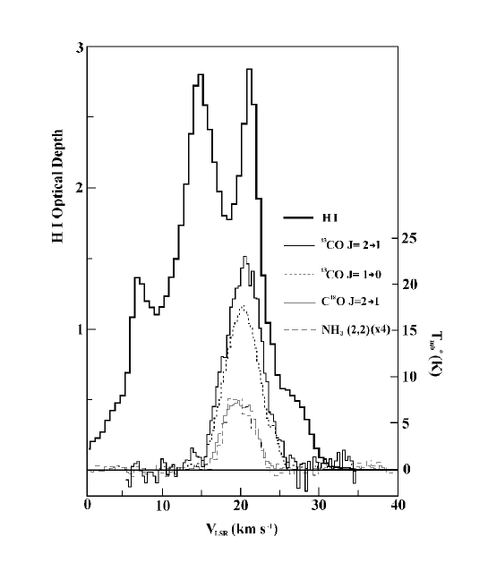
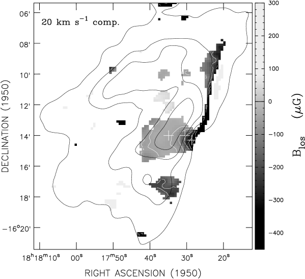
Figure 4: An H i optical depth profile (present work) and ¹³CO, C¹⁸O, and NH₃ emission profiles from Stutzki et al. 1988 toward the position $18^{\rm h}17^{\rm m}30.6^{\rm s}$, ${-16}\arcdeg 14\arcmin 00\arcsec$ (also known as position (-60,-30) in Stutzki et al.) .

Figure 5: Greyscale map of $B_{los}$ for the 20 km s^-1 component with white contours at $-$400, $-$300, $-$200, $-$100, and $-$50 $\mu$G. The 21 cm 1, 5, 10, and 20 Jy beam^-1 continuum contours are shown in black. The three white + symbols show the positions of the profiles shown in Figs. 7 a, b, c .

[fig20prof.eps]Representative fits at three positions for the 20 km s^-1 component (17.0 to 24.6 km s^-1). The upper panels show Stokes I profiles (dashed histogram), and the bottom panels show Stokes V profiles (solid histogram) with the fitted derivative of Stokes I shown as a smooth dashed curve. In the upper and lower panels, the velocity range used in the fit is denoted by solid or heavier lines. The value of $B_{los}$ fit for each position and its calculated error are given at the top of each plot. (a) Position $18^{\rm h}17^{\rm m}35^{\rm s}$, ${-16}\arcdeg 14\arcmin 00\arcsec$. (b) Position $18^{\rm h}17^{\rm m}30.6^{\rm s}$, ${-16}\arcdeg 14\arcmin 00\arcsec$, or position (-60, -30) from Stutzki et al. (1988). (c) Position $18^{\rm h}17^{\rm m}28.5^{\rm s}$, ${-16}\arcdeg 14\arcmin 16\arcsec$, or position (-90, -45) from Stutzki et al. (1988) .

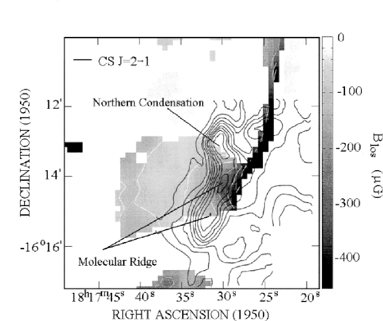
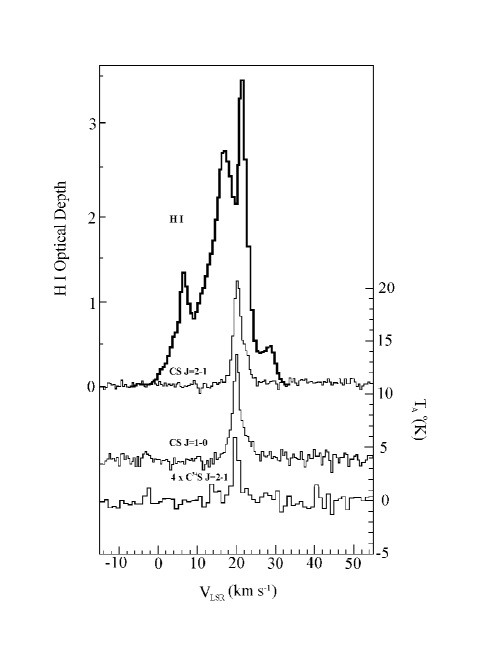
Figure 6: Magnified greyscale of the $B_{los}$ for the 20 km s^-1 component with black CS $J=2\rightarrow~{}1$ contours from Wang et al. (1993) superimposed. The white $B_{los}$ contours are at $-$400, $-$300, $-$200, $-$100, and $-$50 $\mu$G. Notice the spatial coincidence between the highest values of $B_{los}$ and the molecular ridge traced by CS emission .

[crywang5.eps]An H i optical depth profile (present work) and emission spectra from several CS transitions toward the molecular ridge ($18^{\rm h}17^{\rm m}32.4^{\rm s}$, ${-16}\arcdeg 15\arcmin 06\arcsec$) from Wang et al. (1993). See also Fig.8 .

3.3.2 Magnetic Fields Derived for the Blended 11$-$17 km s^-1 Components

figu10 figu11

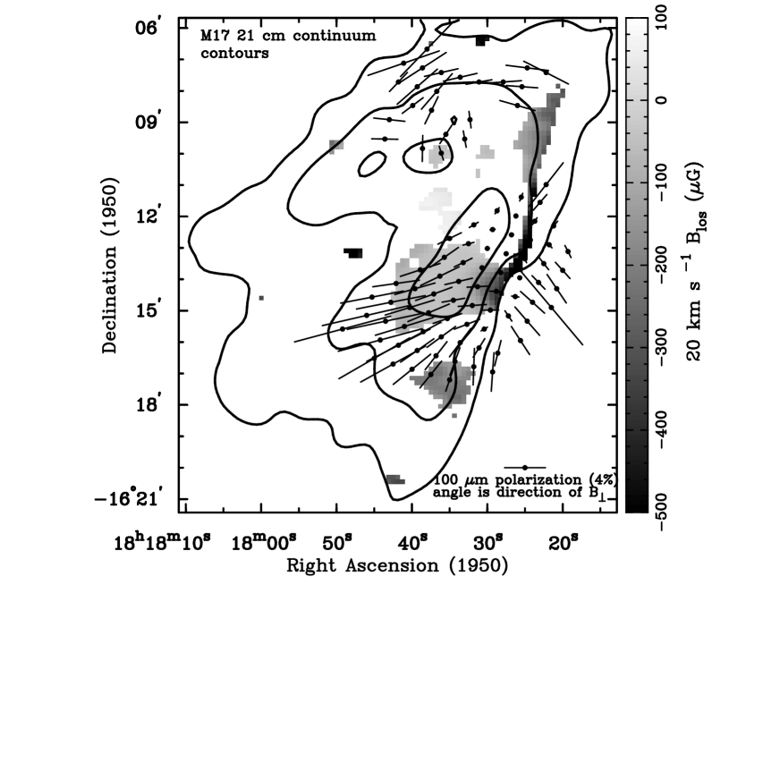
Figure 11: Greyscale of the 20 km s^-1 $B_{los}$ overlaid with the 1, 5, 15 Jy beam^-1 contours from our 21 cm continuum, and the 100 $\mu$m linear polarization vectors from Dotson (1996). The position angle of the 100 $\mu$m polarization vectors indicates the direction of $B{{}_{\bot}}$, which is perpendicular to the observed linear polarization direction .

Strong, primarily positive magnetic fields were also detected in blended velocity components between 11 to 17 km s^-1. A map of this magnetic field is shown in Fig. 10 and the fit to a few representative pixels can be seen in Figs. 11a, 11b, and 11c. There are four main regions of significant $B_{los}$ for this blended component which appear primarily in the northeastern, north central and western parts of the map. The center velocity of this component (defined by the velocity at which the derivative changes sign) is somewhat different in each of these regions. They range from 14.4 km s^-1 in the northeast (Fig. 11a), 13.7 km s^-1 in the central northern feature (Fig. 11b), 14.0 km s^-1 in the northwest (Fig. 11c) and 12.4 km s^-1 in the southwest. One interesting feature of the $B_{los}$ for this component is that the direction of the field changes from positive (away from the observer) to negative and back to positive across the map from east to west (this trend can be seen in the fits shown in Figs. 11 a, b, c). $B_{los}$ in the northwestern feature reaches values as high as +550 $\mu$G with $S/N_{B}$ as high as 14.

Evidence for molecular gas near this velocity has been observed in a number of species. For example greGreaves, White, & Williams (1992) reported a velocity component in this range in their ¹²CO $(3\rightarrow 2)$ and ¹³CO $(3\rightarrow 2)$ spectra. Their component shifts from 12 km s^-1 in the southeast to 16 km s^-1 further to the southwest of their field of view (the eastern portion of their maps overlaps the the western side of our maps). The positions where their low velocity component is centered at 12 km s^-1 corresponds to the southwestern region of our magnetic field map where the H i line center is 12.4 km s^-1. rainRainey et al. (1987) and stut88Stutzki et al. (1988) also identified emission in this velocity range in ¹²CO $(3\rightarrow 2)$ and ¹²CO $(2\rightarrow 1)$, respectively. masMassi et al. (1988) observed that two of their seven NH₃ clumps near M17-UC1 have velocities of 15.5 km s^-1 and stut88 Stutzki et al. (1988) observed 31 C¹⁸O clumps (out of 180) in the 11$-$17 km s^-1 velocity range .

figu12

In addition to molecular gas, there is also [C ii] 158 $\mu$m emission at a velocity of $\sim$ 17.8 km s^-1 (borBoreiko et al. 1990). [C ii] 158 $\mu$m is an important tracer of PDR’s and should exist in the same zone of a PDR as H i gas. The precise spatial correlation between these two atomic species for M17 is unknown. However, the low resolution (3.4) map of [C ii] 158 $\mu$m obtained by matMatsuhara et al. (1989) does seem to follow the same morphology as our summed N_HI/T_s (see Fig. 4a). A profile from one pixel at the [C ii] 158 $\mu$m peak from borBoreiko et al. (1990; spatial resolution 43) and H i are shown in Fig. 12. The [C ii] 158 $\mu$m profile appears to have a component at a lower velocity than their lowest reported velocity of 17.8 km s^-1. The authors noted that there may have been some contamination from emission in the reference beam at this position. The possible significance of a lower velocity [C ii] 158 $\mu$m component will be discussed again in §4.1.3.

3.3.3 Magnetic Field Detections at $\sim$ 3.4, 6.7, and 27 km s^-1

Line of sight magnetic field detections were also made for three other velocity components. A significant $B_{los}$ was measured in the velocity range $-$2.4 to 4.0 km s^-1 with the line center at $\sim 3.4$ km s^-1. This detection is interesting because the $S/N_{B}$ in the southeastern region is as high as 10 and there is a rapid change in $B_{los}$ from negative to positive values along the northwestern border with M17 SW. This abrupt change in field direction corresponds to the behavior of the $B_{los}$ measured in the 20 km s^-1 component in this same region. The line of sight fields in this component range from $\sim$ $-$200 to +100 $\mu$G.

Detections were also made in the velocity range from 4.1 to 10.5 km s^-1 with a center velocity of $\sim 6.7$ km s^-1 and the maximum

Figure 8: Same as Fig. 7 a,b,c except the range of velocities used in the fit for $B_{los}$ was 11$-$17 km s^-1. (a) Northeastern position $18^{\rm h}17^{\rm m}40.6^{\rm s}$, ${-16}\arcdeg 10\arcmin 15\arcsec$ (white + symbol in Fig. 10). (b) North central position $18^{\rm h}17^{\rm m}35.6^{\rm s}$, ${-16}\arcdeg 10\arcmin 51\arcsec$ (white + symbol in Fig. 10), and (c) Northwestern position $18^{\rm h}17^{\rm m}28.7^{\rm s}$, ${-16}\arcdeg 09\arcmin 12\arcsec$ (black + symbol in Fig.10). Notice how the sign of the field changes as you move from east to west across the map .

$S/N_{B}=6.4$. Reliable measurements of $B_{los}$ in this H i component range from $\sim$ $-$125 to +100$\mu$G. The regions of significant $B_{los}$ measured for this component do not particularly correspond to the morphology of the 21 cm continuum emission of M17. In fact the highest fields and concentration of H i in this velocity range are to the southeast. One interesting possibility is that there is a connection between H i measured in this velocity range and the 7 km s^-1 and the cold cloud observed by riegRiegel & Crutcher (1972) at 21 cm over a large region toward the galactic center including the direction of M17. cru84Crutcher & Lien (1984) estimate that this cold cloud ($\sim$20 K) must be located within 150 pc of the sun.

A sparse $B_{los}$ was also detected in the range 24.7 to 33.0 km s^-1 with a center velocity of $\sim 27$ km s^-1 and maximum $S/N_{B}$=6. The $B_{los}$ in this H i component ranges from $\sim$ $-$200 to +100 $\mu$G. A component in this velocity range was also observed by gre Greaves et al. 1992 in ¹²CO $(3\rightarrow 2)$ and ¹³CO $(3\rightarrow 2)$ emission. The ratio of these two species’ intensity seems to indicate the presence of a distinct cloud at this velocity.

4 DISCUSSION

4.1 Proposed Origin of Magnetic Field Components

4.1.1 General Nature of the M17 Region

meiMeixner et al. (1992) suggest that the coincidence of part of their [O i] 63 $\mu$m map with the radio continuum emission indicates that hot ionized gas from the H ii region is carving a bowl into the molecular cloud to the southwest (M17 SW). The symmetry axis of the bowl lies in the plane of the sky, and the overlapping [O i] 63 $\mu$m emission arises from a PDR on the front and/or back sides of the bowl. The bottom of the bowl (at the southwestern edge of the southern bar) is the portion of the H ii region-molecular cloud interface viewed edge$-$on. Further evidence of a bowl$-$like morphology is the high visual extinction toward the southern bar which presumably arises from the front side of the bowl. gulGull & Balick (1974) also suggest a bowl morphology based on the double peaks separated by $\sim$ 20 km s^-1 in their H76$\alpha$ radio recombination line data. (Also, see gouGoudis & Meaburn 1976.) These two recombination line velocity components are thought to arise from streaming motions of newly-ionized gas at the front and back sides of the bowl.

In many ways, this M17 interface model resembles the interface region between the Orion nebula and the molecular cloud behind it. For Orion, the interface lies in the plane of the sky with the ionizing stars directly in front of it. For M17, the geometry is turned by 90$\arcdeg$. The interface layer is perpendicular to the plane of the sky, with the ionizing stars offset to the northeast. The densest accumulation of ionized gas in M17 lies along the “working surface” near the ionization front. Therefore, the brightest region in the M17 continuum map, the southern bar, does not coincide in the sky with the ionizing stars as it does for the Orion nebula.

The clumpiness of the M17 interface has been observed in many molecular species (§1). It seems to closely resemble the scenario discussed by bert96Bertoldi& Draine (1996), whereby dense clumps are slowly photodissociated by a nearby H ii region. In this case the H ii region is partially embedded in (and partially obscured by) a bowl of clumpy neutral gas. The H i gas associated with M17 can arise, in principle, anywhere in front of the source. Our data suggest that the 20 km s^-1 component originates primarily in the edge$-$on portion of the bottom of the molecular bowl. In this model the 20 km s^-1 H i arises from molecular gas that been partially photodissociated but otherwise dynamically undisturbed (unshocked). On the other hand, the H i data for the 11$-$17 km s^-1 component supports the idea that it arises from photodissociated, shocked gas from the front side of the molecular bowl which is streaming toward us. The association of different H i absorption components with shocked and unshocked gas has also been suggested for S106 (Roberts et al. 1995) and W3 (Roberts et al. 1993). Evidence supporting this picture for M17 is given in §4.1.2 and 4.1.3.

4.1.2 The Nature of H i Gas at 20 km s^-1

The velocity range of the 20 km s^-1 H i component (17 to 24.6 km s^-1) includes most of the molecular gas in the M17 region (e.g rainRainey et al. 1987 and §3.3.1). Therefore, H i components in this range are likely to be closely associated with the bulk of the M17 molecular gas. Such an association is particularly clear toward the molecular ridge (see Fig. 8) where the center velocity of the 20 km s^-1 H i component closely matches that of a variety of molecular lines, including high density tracers such as CS (Figs. 5, 9, and 12). This H i component is also relatively narrow (3-5 km s^-1), and its center velocity changes little with position along the interface region. Therefore, it most likely originates in quiescent gas that is dynamically unaffected by the H ii region. Much of this quiescent gas must lie in the edge-on H ii region$-$M17 SW interface region at the bottom of the bowl described by meiMeixner et al. (1992). Hence the concentration of 20 km s^-1 H i gas and high $B_{los}$ ($\sim-450$ $\mu$G) near the interface region (Figs. 3, 4b, 6, and 8).

figu13

Further indication of the association between H i and molecular gas comes from similarities in their spatial distribution near the molecular ridge. Fig. 13 (upper panel) shows the relative intensity of several species along the NE-SW strip scan defined by stut88Stutzki et al. (1988). The strip lies perpendicular to the interface region and cuts across it (ionizing radiation propagates from left to right). As shown in the figure, the increase in the 20 km s^-1 $N_{HI}/T_{s}$ and $B_{los}$ (lower panel) matches well the increase in ¹²CO line strengths to the right of the H ii region. In fact, $N_{HI}/T_{s}$, ¹²CO$(2\rightarrow 1)$, and ¹²CO$(7\rightarrow 6)$ peak outside of the H ii region as expected for an interface region viewed edge on. Note that the actual peak in $N_{HI}/T_{s}$ for the 20 km s^-1 component is not defined by our data since we cannot detect H i absorption beyond the continuum source.

Notice that the integrated [C ii] 158 $\mu$m emission, also shown in Fig. 13, peaks inside (to the left of) the rise in the 20 km s^-1 $N_{HI}/T_{s}$. In a simple planar PDR model, [C ii] 158 $\mu$m emission coincides with H i and with molecular gas up to $A_{v}=2-4$ mag. (See review byholl90Hollenbach, 1990.) However, the higher velocity resolution [C ii] 158 $\mu$m profiles of borBoreiko et al. (1990) reveal the presence of several [C ii] 158 $\mu$m velocity components. An examination of these profiles suggests that the $\sim$ 20 km s^-1 [C ii] 158 $\mu$m component alone peaks further into the molecular cloud than the integrated [C ii] 158 $\mu$m emission plotted in Fig. 13. Also, note that the rise in the 11$-$17 km s^-1 $N_{HI}$/$T_{s}$, plotted in Fig. 13 (lower panel), peaks to the left of the 20 km s^-1 $N_{HI}/T_{s}$ in a similar manner to the integrated [C ii] 158 $\mu$m emission. In fact, the contribution of lower velocity [C ii] 158 $\mu$m emission to the integrated emission plotted in Fig. 13 may explain why it seems to peak to the left of the 20 km s^-1 $N_{HI}/T_{s}$. Apparently, H i and [C ii] 158 $\mu$m gas is more broadly distributed along the strip in Fig. 13 than is the gas at 20 km s^-1 alone. This shows that absorbing H i gas lies on the near side of the bowl, not just at the bottom.

The close association between H i gas near 20 km s^-1 and the molecular ridge region could arise in at least two ways. For one, the H i may be well mixed with and a minor constituent of the molecular gas. In such a case, the Zeeman effect near the ridge (Fig. 8) is directly representative of magnetic fields in the molecular gas. A second possibility is that the absorbing H i near 20 km s^-1 is confined to a thin photodissociated shell about the molecular ridge or to thin shells surrounding a multitude of molecular clumps within the ridge. In this case, the H i Zeeman effect is also representative of the magnetic field in the molecular gas if the H i is photodissociated but dynamically undisturbed H₂.

In either case, the H i Zeeman effect near the

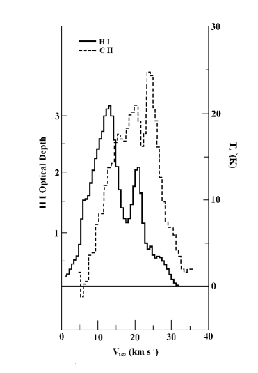
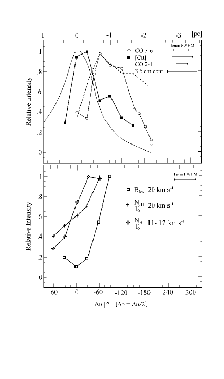
Figure 9: An H i optical depth profile (present work) and a [C ii] 158 $\mu$m spectra from Boreiko et al. (1990) for the position of the Stutzki et al. (1988) [C ii] 158 $\mu$m “peak” $18^{\rm h}17^{\rm m}32.5^{\rm s}$, ${-16}\arcdeg 13\arcmin 42\arcsec$, or (-30, -15) .

Figure 10: Upper panel : Distribution of the relative intensity of 3.5 cm continuum, CO ($7\rightarrow 6$), CO ($2\rightarrow 1$) and [C ii] 158 $\mu$m across the H ii region$-$ M17 SW interface following the NE-SW strip scan observed and plotted by Stutzki et al. (1988). Lower panel : Relative intensity of the 20 km s^-1 $N_{HI}/T_{s}$, 20 km s^-1 $B_{los}$, and 11$-$17 km s^-1 $N_{HI}/T_{s}$ for the same positions as the upper panel. The peak positions for the 20 km s^-1 $N_{HI}/T_{s}$ and 20 km s^-1 $B_{los}$ do not necessarily represent true maxima, due to the loss of continuum power as the strip is transversed to the west. Notice that the 11$-$17 km s^-1 $N_{HI}/T_{s}$ distribution along this strip is similar to the distribution of [C ii] 158 $\mu$m emission (east of the continuum power drop-off), while the 20 km s^-1 $N_{HI}/T_{s}$ and 20 km s^-1 $B_{los}$ peak further west .

molecular ridge must arise in relatively dense gas if approximate equilibrium exists between the magnetic energy density and that associated with non-thermal motions in the gas. Such an equilibrium was suggested by my88a my88bMyers & Goodman (1988a, 1988b) on the basis of limited observational data. In such a case, the gas density is given by

$$n_{eq}=\left[\frac{B_{avg}}{0.4\Delta v_{NT}}\right]^{2}{\rm cm}^{-3},$$ (2)

where $n_{eq}$ is the proton density, $B_{avg}$ is the average field strength ($\mu$G), and $\Delta v_{NT}$ is the FWHM contribution to the line width from non-thermal motions (km s^-1; see also §4.3). As an example we apply this equation to the position of Fig. 5 ($\sim 15\arcsec$ east of molecular ridge). At this position, $\Delta v\approx 4$ km s^-1, and $B_{avg}$ $\;\stackrel{{\scriptstyle>}}{{\sim}}\;$ 200 $\mu$G. If $T_{s}=T_{K}=50$ K (as estimated by berginBergin et al. 1994 from ¹²CO observations), $\Delta v_{NT}$ = 3.7 km s^-1 and $n_{eq}\raisebox{-2.15277pt}{$\;\stackrel{{\scriptstyle>}}{{\sim}}\;$}\/2\times 10^{4}$ cm^-3. This estimate of the local density in which the H i Zeeman effect arises is conservative since the actual field strength $B_{avg}$ almost certainly exceeds $B_{los}$ and $n_{eq}\propto B_{avg}^{2}$. This value for $n_{eq}$ based on $B_{los}$ is also in excellent agreement with the value of $n_{eq}\approx 6\times 10^{4}$ cm^-3 calculated toward M17 SW by Goldsmith, Bergin, & Lis (1997) using C¹⁸O column densities and average line widths. However, at the position cited here, $N_{HI}/T_{s}$ in the 20 km s^-1 component is only 3 $\times 10^{19}$ cm^-2K, so $N_{HI}=1.5\times 10^{21}$ cm^-2 for $T_{s}=$50 K. A typical scale length for H i absorption features in the plane of the sky is of order 2 pc (3$\arcmin$ at 2.2 kpc). If the same scale length applies along the line of sight, then $n_{HI}$ $\approx$ 250 cm^-3. That is, if the H i Zeeman effect arises in gas at a density of order $n_{eq}$, then the H i could be about only a 1% constituent of largely molecular gas. This possibility exists because the $N_{H_{2}}$ estimated by stut88Stutzki et al. (1988) and Goldsmith et al. (1997) near this direction ($\approx 2-8\times 10^{23}$ cm^-2) is about 100 times higher than $N_{HI}$. Alternatively, H i might not be mixed with H₂ but confined to thin sheets or very dense, thin atomic envelopes surrounding the multitude of molecular clumps which have been observed in the interface region (see §1). Note that this would still require the H i gas to occupy about 1% of the line of sight in the absorbing region. These two cases are the same ones cited above to explain the close association of H i gas with molecular gas in the ridge.

4.1.3 The Nature of H i Gas at 11$-$17 km s^-1

The morphology and velocity structure of gas between 11$-$17 km s^-1 suggest that it also lies very close to the H ii region on the near side of the bowl and that it has been shocked and accelerated away from the ionized gas. The 11$-$17 km s^-1 gas is primarily distributed in an arc that partially encircles the northern and southern bars of the H ii region (Figs. 3, 4c). This arc of H i column density corresponds well with a similar arc structure apparent in ¹²CO($3\rightarrow$2) emission mapped by rainRainey et al. (1987) in the velocity range 14$-$20 km s^-1. This morphology suggests a very close relationship between gas in the 11$-$17 km s^-1 velocity range and the H ii region. The gas is blue-shifted by 2-8 km s^-1 relative to the H ii region center velocity of 19 km s^-1 (joncJoncas & Roy 1986). Also, H i in this velocity range shows complex velocity structure with numerous components appearing at various positions across the source (Figure 2, 11 a, b, c). This complicated velocity field and magnetic field reversal (see §3.3.2) suggest that gas in the 11$-$17 km s^-1 range lies in an interface zone that has been dynamically affected by interactions with the H ii region, unlike the 20 km s^-1 component discussed in §4.1.2.

Overall, the association between atomic and molecular gas in this velocity range is much less clear than it is at 20 km s^-1 near the western interface region. This could in part be due to fact that few high resolution molecular observations have mapped the northern regions of M17. However, judging from ¹²CO $J=1\rightarrow$0, ¹²CO$J=3\rightarrow$2, and ¹³CO observations (lad76Lada 1976; rainRainey et al. 1987) which all show components in this velocity range, the density of molecular material in this region is low compared to the western interface. Toward the northern bar in particular, where the 11$-$17 km s^-1 H i magnetic fields are high (see §3.3.2), there is not always a molecular counterpart in the 11$-$17 km s^-1 velocity range. In fact, for the positions shown in Figs. 11a and 11b there is no evidence of molecular gas. Such a variable ratio of atomic to molecular gas might be expected if gas in this velocity range has been subjected to a widely variable degree of dissociation in the interface region.

Although molecular column densities are low in the 11$-$17 km s^-1 range, H i field strengths are very high, reaching values of over +500 $\mu$G (Fig. 10). Therefore, the assumption of equilibrium between magnetic and non-thermal energies leads to conclusions similar to those for gas near 20 km s^-1 (§4.1.2). That is, $n_{eq}\raisebox{-2.15277pt}{$\;\stackrel{{\scriptstyle>}}{{\sim}}\;$}\/10^{4}$ cm^-3, and $n_{HI}$ along the line of sight is about two orders of magnitude less than $n_{eq}$. Yet the scarcity of molecular gas at positions of high field strength means that H i at these positions cannot exist as a minor constituent in a largely molecular region. If the H i alone is to exist at a density near $10^{4}$ cm^-3, it must reside in one or more thin layers that occupy only about 1% of the path length through the H i absorbing region. That is, the absorbing H i gas is distributed in a very clumpy fashion along the line of sight. This conclusion is consistent with numerous other indications of a highly clumped medium in the M17 region (§1). Most likely, the absorbing H i gas is shocked, photodissociated gas lying in thin interface regions about ablating neutral clumps. The clumps, in turn, lie within mostly ionized gas, like the clumps modeled by Bertoldi & Draine (1996) or the clumps identified by felFelli et al. (1984) in high resolution M17 radio continuum maps. In these clumps, the pressure of the ionized gas drives a shock front into the neutral medium. Therefore, a rough equivalence between the thermal energy density of the ionized gas and the magnetic energy density in the adjacent compressed atomic region is expected. Evidently, this is the case. If the M17 ionized gas has a temperature of 8000 K (subSubrahmanyan & Goss 1996) and a density of $10^{4}$ cm^-3 (felFelli et al. 1984), then its thermal energy density is equivalent to the magnetic energy density in the thin H i layers for B $\approx$ 500 $\mu$G.

Several reasons exist to expect H ii region driven motions of a few km s^-1 near M17. Observationally, rainRainey et al. (1987) fit their ¹³CO data on molecular clumps near the southern bar to a geometric expansion model about Kleinemann’s star (Fig. 1). They obtain an expansion velocity of $\approx$ 11 km s^-1 about this star. Radio and optical recombination line observations often reveal split profiles shifted by about $\pm 8$ km s^-1 from the H ii region rest velocity (gulGull & Balick 1974; joncJoncas & Roy 1986). Theoretically, bert96Bertoldi& Drain (1996) estimated the shock-induced acceleration expected in the Orion nebula PDR, obtaining a value of 3 km s^-1. This value is somewhat sensitive to the ratio of post to pre-shock density, taken by bert96 Bertoldi& Draine (1996) as 2. If the ratio for M17 is 4, as suggested by the ratio of the square of the ¹²CO $(7\rightarrow 6)$ (5 km s^-1) line width (harHarris et al. 1987) to the square of the CS $(2\rightarrow 1)$ line width (2.5 km s^-1, wanWang et al. 1993), then the shock induced acceleration is increased to 6 km s^-1. Also, bert89Bertoldi) and bert90Bertoldi & McKee (1990) discuss a rocket effect upon ablating clumps of neutral gas exposed to ionizing radiation. They estimate that rocket acceleration should amount to a clump velocity of 5$-$10 km s^-1 under typical circumstances. These estimates of shock speed, agree quite well with the 2$-$8 km s^-1 blueshift of the 11$-$17 km s^-1 componets.

4.2 Comparison of 20 km s^-1 $B_{los}$ Field Morphology with Polarimetry Studies

A number of studies have been made of linear polarization toward M17. These include polarization at optical and near IR wavelengths from grain absorption and polarization in the far IR from grain emission. (See references cited by dotDotson 1996.) Such studies reveal the position angles of the magnetic field in the plane of the sky ($B_{\bot}$), but they yield little if any information about field strengths. Therefore, they compliment Zeeman effect studies, assuming the linear and circular polarization arise in the same regions. In general, field directions inferred from grain absorption do not agree with those inferred from grain emission. Very likely, this disprepancy results from the different regions sampled by each technique, with grain emission data more likely representative of the field directions inside M17 SW (goodGoodman et al. 1995).

figu14

The study of polarized 100 $\mu$m dust emission by dotDotson (1996) provides the most comprehensive available data set for comparison with H i Zeeman effect results. In figure 14 we present a map of the position angle of the transverse magnetic field $B_{\bot}$ from dotDotson (1996) overlaid on our $\sim$20 km s^-1 $B_{los}$ grayscale. The resolution of the dotDotson study (35$\arcsec$) is comparable to that of the H i data. Also, the 20 km s^-1 H i component likely samples at least part of the molecular ridge (§4.1.2) as does the 100 micron emission. A principal conclusion of the dotDotson study is that the M17 magnetic field shows a significant degree of spatial coherence across M17. The H i Zeeman data for the 20 km s^-1 component corroborates this result (Figs. 6, 8). Moreover, the eight-fold increase in $B_{los}$ from east to west toward the molecular ridge (Fig. 8) is matched by a decrease in fractional linear polarization from about 4% to 1%. Along this same line the field has a nearly constant position angle (predominantly east-west). Since $B_{los}$ is perpendicular to both to the transverse magnetic field and the 100 $\mu$m linear polarization vectors, one might expect to see a correlation between regions of maximum $B_{los}$ and minimum 100 $\mu$m polarization.

One obvious interpretation of the IR and H i Zeeman data is that the magnetic field lines curve into the line of sight as one approaches the molecular ridge from the east. In such a case, $B_{los}$ may be a close approximation to the total field strength in the region of the molecular ridge sampled by H i. Since the H i must lie in front of the H ii region, the field lines in this picture wrap around the H ii region on the front side of the bowl, becoming more aligned with the line of sight at the bottom of the bowl as they pass through the molecular ridge. This geometry is consistent with the inferences made by dotDotson from the linear polarization data alone. The origin of the field curvature may lie in the process of gravitational contraction that formed the molecular ridge, gathering an initially uniform field along the line of sight into an hourglass shape with the ridge at its waist. An hourglass shaped field structure was also suggested for the W3 region by Roberts et al. (1993), although for this source, the axis of the hourglass is nearly in the plane of the sky rather than along the line of sight. Alternately, the present geometry of the M17 field may represent the bending effects of the H ii region as it expands into the molecular cloud deforming a field originally along the line of sight into a bowl-like shape.

It should be noted that the occurrence of decreasing linear polarization toward the the 100 $\mu$m flux and column density maxima could result from effects other than a true minimum in the transverse magnetic field component. For example, optical depth effects, dust properties, grain alignment efficiency, or some combination of these can cause a decrease in the linear polarization independent of the magnetic field. On the other hand, the magnetic field itself could simply be more tangled in higher density regions (jonJones, Klebe, & Dickey 1992; my91Myers & Goodman 1991). In addition, the 760 $\mu$m polarimetry by valVallée & Bastien (1996) does not show a minimum in the linear polarization in this region of the molecular ridge. However, the 760 $\mu$m polarization arises from cooler dust grains which could be spatially distinct along the line of sight from those emitting at 100 $\mu$m. Future polarimetry of this region at an intermediate wavelength from ISO and

higher resolution H i Zeeman results may help to clarify this issue.

4.3 Magnetic Energy vs. Turbulent and Gravitational Energy

The magnetic field in a cloud can be separately described in terms of a static component $B_{S}$ and a time-dependent or wave component $B_{W}$. The static component connects the cloud to the external medium and also determines the total magnetic flux through the cloud, while the wave component is associated with MHD Alfvén waves in the cloud (e.g. ArArons & Max 1975). Although the static component of the field can only provide support to the cloud perpendicular to the field lines, the turbulent or wave component can provide 3-D support (mck95 Mckee & Zweibel 1995, also see references therein). If a cloud is threaded by $\Phi_{B}=\pi R^{2}$$B_{S}$, it can be completely supported perpendicular to $B_{S}$ if its mass does not exceed the magnetic critical mass $M_{\Phi,crit}\approx 0.13G^{-{1/2}}\Phi_{B}$ (mou76Mouschovias & Spitzer 1976). This criterion leads directly to the observationally relevant relation

$$B_{S,crit}\approx 5\times 10^{-21}N_{p}~{}\mu{\rm G},$$ (3)

where $N_{p}$ is the average proton column density of the cloud. If $B_{S}$ $>$ $B_{S,crit}$ (i.e. $M<M_{\Phi}$), then the cloud is supported by $B_{S}$, it is magnetically subcritical, and further evolution of the cloud perpendicular to the field can only occur via ambipolar diffusion. If $B_{S}$ $<$ $B_{S,crit}$, (i.e. $M>M_{\Phi}$), then $B_{S}$ cannot fully support the cloud, the cloud is magnetically supercritical, and internal motions must supply additional support if the cloud is stable. In this case, further evolution of such a cloud will be controlled in part by processes that create and dissipate internal motions.

As discussed above, the second type of support provided by magnetic fields arises from Alfvén waves generated in a turbulent velocity field. The fluctuating or wave component of the magnetic field $B_{W}$ organizes supersonic (but sub-Alfvénic) motions in the gas so that highly dissipative shocks do not occur. Theoretical studies suggest that equipartition between the wave’s kinetic and magnetic potential energy densities almost certainly exists in molecular clouds (zweZweibel & Mckee 1995, and references therein). That is $3/2\rho\sigma_{NT}=$ $B_{W}$${}^{2}/8\pi$ where $\sigma_{NT}$ is the non-thermal component of the velocity dispersion, which is assumed to arise exclusively from Alfvén waves. These assumptions lead to the equivalent of equation (2) for $B_{W}$, that is,

$$B_{W}\approx 0.4\Delta v_{NT}n_{p}^{1/2}~{}\mu{\rm G},$$ (4)

where $\Delta v_{NT}$ is the non-thermal line width (FWHM) and $n_{p}$ is the proton density. Since Zeeman effect measurements are generally sensitive to large scale fields (on the order of the beam size), they are expected to be better indicators of $B_{S}$ than of $B_{W}$. Therefore, the formal usefulness of comparing equation (4) for $B_{W}$ to Zeeman observations ($B_{los}$) is not clear. However, limited observational comparisons of Zeeman measurements with the $B_{W}$ predicted from equation (4) show that there may also be approximate equipartition between the wave’s kinetic and static magnetic energy densities in molecular clouds; ie. $\sigma_{NT}\approx 1/3v_{A}$, where $v_{A}^{2}=$$B_{S}$${}^{2}/4\pi\rho$, or equivalently $B_{S}$$\approx$$B_{W}$ (my88a my88bMyers & Goodman 1988a, 1988b; Bertoldi & Mckee 1992; mou95Mouschovias & Psaltis 1995). In any case it is worth noting that $B_{W}$ must be $\leq$ $B_{S}$ to prevent the formation of super-Alfvénic shock waves, which are highly dissipative (mck95McKee & Zweibel 1995).

We can assess the role of magnetic fields in the support of M17 SW from our H i Zeeman measurements combined with other measurements of the clouds basic properties. Goldsmith, Bergin, & Lis (1997) estimate that the mass of the M17 SW is $M_{core}=1.2\times 10^{4}~{}{\rm M_{\odot}}$ (including helium) on the basis of their C¹⁸O maps. Using the geometric mean of the extent of their M17 SW C¹⁸O maps (1.9 pc $\times$ 2.2 pc) $\sim 2$ pc as the $diameter$ of the core region, and their integrated C¹⁸O column density, we estimate $<$$N_{p}$$>\approx 4\times 10^{23}$ cm^-2 and $<$$n_{p}$$>\approx 6\times 10^{4}$ cm^-3 (assumes filling factor of 1). Although $\Delta v_{NT}$ is often estimated from the $\Delta v_{FWHM}$ of optically thin lines, we believe a more accurate estimate for the internal motions of the M17 SW core as a whole comes from the velocity dispersion of the center velocities of the clumps themselves. stut90Stutzki & Güsten (1990) identified 180, $\sim 0.1$ pc C¹⁸O clumps in M17 SW and provide center velocities for each. The dispersion of these center velocities is 2.7 km s^-1, equivalent to $\Delta v_{NT}$ = 6.3 km s^-1. From these parameters and equations (3) and (4), $B_{S,crit}$$\approx 2000$ $\mu$G and $B_{W}$$\approx$ 620 $\mu$G. These estimates indicate that (1) unless the static field is four or more times higher than our maximum values for $B_{los}$ (500 $\mu$G), then M17 SW as a whole is magnetically supercritical and (2) the estimate for $B_{W}$ is in good agreement with our highest values for $B_{los}$. Therefore, the evolution of the M17 SW core is not entirely controlled by $B_{S}$ and ambipolar diffusion, and internal motions must play a role in its support and dynamics. Note that these estimates are not necessarily valid for individual clumps within the core (bert92Bertoldi& McKee 1992).

Another perspective on cloud support can be gained from a simplified form of the virial theorem that simultaneously takes into account magnetic effects from $B_{S}$ and $B_{W}$ (but not external pressure or rotation). This form is

$$\mid{\cal W}\mid={\cal M}_{S}+3{\cal T},$$ (5)

where ${\cal W}$ is the gravitational energy term, ${\cal M}_{S}$ is the magnetic energy associated with $B_{S}$, and 3${\cal T}$ is the energy contribution from all internal motions including the magnetic wave energy produced by $B_{W}$ (See, for example, Mckee et al. 1993 for a more detailed description of these terms.). Note that 2T, in the non-magnetic virial equation, has been replaced by 3T because equipartition between internal motions and Bw adds an additional term T to the energetics of the cloud. mck93McKee et al. (1993) explain why virtually all self-gravitating clouds must be close to dynamically critical since their internal pressures would otherwise be comparable to external pressures, contrary to observation. If M17 SW is dynamically critical, that is, on the verge of collapse, then the virial equation above can be rewritten in the form

$$B_{S}\approx B_{S,crit}[1-(3{\cal T}/{\mid\cal W\mid})]^{1/2}.$$ (6)

Given the M17 SW cloud parameters estimated at the beginning of this section, ${\cal T}$/$\mid$${\cal W}$$\mid$ $\approx$ 0.3, so $B_{S}$ $\approx(1/3)$$B_{S,crit}$ $\approx 660$ $\mu$G, and $M_{\Phi}\approx 1/3M_{core}$. Given the inevitable errors in estimating virial terms, these values are quite uncertain. However, they can be regarded as a possible equilibrium model for the energetics of the M17 SW core. In this model, internal motions in the core are sub-virial since ${\cal T}$/${\cal W}$ $<$ 1/2, and the cloud is magnetically supercritical. That is, the cloud is supported in part by internal motions, with the remainder of the support coming from $B_{S}$. Moreover, the magnitude of $B_{S}$ in this model is comparable to $B_{W}$ (620 $\mu$G), so that the magnetic support provided by the static and wave components of the field are comparable. This suggests that $B_{S}$$\approx$$B_{W}$ is a good assumption for M17 SW (see above). Although our estimate for $B_{S}$ using this model is quite close to the highest measured values of $B_{los}$ ($\approx 500$ $\mu$G), this agreement must be considered somewhat fortuitous since estimates of $B_{S}$ are very sensitive to uncertainties in cloud parameters and, of course, $B_{los}$ is just one component of the field.

Apart from equations (3), (4), and (6), one other method has been used to estimate field strengths in self-gravitating clouds. Letting 2${\cal T}$$=\alpha\mid$${\cal W}$$\mid$ we obtain the following mass estimate:

$$M=\frac{5}{{\rm 8ln2}}~{}\left[\frac{\Delta v_{NT}^{2}R}{\alpha G}\right],$$ (7)

where $\alpha$ parametrizes the extent to which a magnetic field is needed to support the cloud, ie. $\alpha<1$ for clouds in which the internal motions are sub-virial. Substituting this estimate for the cloud’s mass into equation (4) we obtain

$$B_{W}=15\alpha^{-1/2}~{}\left[\frac{\Delta v_{NT}^{2}}{R}\right]~{}\mu{\rm G},$$ (8)

where $R$ is in pc and $\Delta v_{NT}$ is in km s^-1. Note that this formulation is similar to those found in my88a my88bMyers & Goodman (1988a, 1988b), mou95Mouschovias & Psaltis (1995) (do not include $\alpha$), and bert92 Bertoldi& McKee (1992) (using $\alpha$). Comparing the mass computed from equation (7), $M=\alpha^{-1}8.5\times 10^{3}{\rm M_{\odot}}$, to the C¹⁸O mass of M17 SW ($1.2\times 10^{4}~{}{\rm M_{\odot}}$), we find $\alpha=0.7$ and $B_{W}$$\approx 740$ $\mu$G, again, remarkably similar to the peak measured value of $B_{los}$. The fact that the field strength predicted by equation (8) is relatively well matched by $B_{los}$ may be another indication that $B_{W}$$\approx$$B_{S}$ for most clouds (see above).

Although formulations similar to equation (8) have often been used to estimate magnetic fields in the literature (see above), we consider equation (6) to yield a somewhat better field estimate, at least in so far as comparison with Zeeman observations are concerned. This is because 1.) if we assume $\alpha=1$ (my88a my88bMyers & Goodman 1988a, 1988b), equation (8) is essentially the same as equation (4), both of which estimate $B_{W}$. There is evidence (this work, and references cited above) that $B_{W}$$\approx$$B_{S}$, but this assertion will require more observational evidence to confirm. 2.) In addition, the assumption that $\alpha$=1, excludes entirely the need for support from $B_{S}$, contrary to our observational Zeeman evidence, ie. $B_{los}$$\approx 500$ $\mu$G. 3.) The inclusion of $\alpha$ in the equation solves this delima, but creates a new one, since the estimate of $\alpha$ only describes the degree of under-virialization in the cloud, and does not distinguish between support from $B_{S}$ and $B_{W}$, while equation (8) is formally an estimate of $B_{W}$ alone. For these reasons equation (6) may be the best method of estimating the magnetic field based on cloud parameters for the purpose of comparison with Zeeman measurements even though all the estimates found here (ie. eq. [4], eq. [6], and eq. [8]) are similar.

5 SUMMARY AND CONCLUSIONS

The H i absorption lines toward M17 show complicated profiles with 5 to 8 distinct velocity components. In general, the highest H i column densities are concentrated toward the H ii region$-$M17 SW boundary. This effect is particularly noticeable in the velocity range of the 20 km s^-1 H i component. A lower limit to the maximum H i column density summed across the whole H i velocity range is N${}_{H_{I}}/T_{s}$= 1.0$\times 10^{20}$ cm^-2. Atomic and molecular emission temperature measurements suggest that $T_{s}$ lies between 50 and 200 K.

A magnetic field has been detected at the same velocity as M17 SW ($v_{LSR}\sim 20$ km s^-1) which peaks steeply toward the M17 H ii region$-$M17 SW interface to values of $B_{los}$= $-$450 $\mu$G. Analysis of this H i component’s line width, along with its velocity and spatial coincidence with molecular density tracers along the M17 SW molecular ridge suggest that it originates in unshocked PDR gas. Comparison of the proton density implied by the observed $B_{los}$ and the 20 km s^-1 H i density show that the H i gas is only a $\sim$ 1% constituent of the gas along the line of sight toward M17. At the same time its distribution along the stut88Stutzki et al. (1988) strip scan across the H ii region$-$M17 SW boundary agrees well with that of molecular gas. Therefore, we suggest that the 20 kms H i gas lies in thin, dense shells around the numerous molecular clumps which have been observed in M17 SW, or it must be well mixed with fairly dense ($1\times 10^{4}$ cm^-3) interclump molecular gas. In addition, the region of maximum $B_{los}$ for this component agrees spatially with a minimum in 100 $\mu$m polarimetry which samples the transverse magnetic field.

Another significant $B_{los}$ was observed in the blended component at 11$-$17 km s^-1 with values reaching $\sim+$ 550 $\mu$G. The morphology of high $N_{HI}$ for this component is quite different from that at 20 km s^-1, with the greatest concentrations found further east and toward the northern parts of the source. From these components’ morphology, line width, and evidence that there is a significant amount of obscuring material on the front side of the M17 H ii region, we suggest that the 11$-$17 km s^-1 components originate in shocked gas that is streaming toward us along the line of sight. Estimates of the shock speeds which can be produced by the M17 H ii region agree well with these components’ blueshift (2$-$8 km s^-1) with respect to the rest velocity of the region. Like the 20 km s^-1 H i component, the 11$-$17 km s^-1 H i gas can only comprise $\sim$ 1% of the line of sight gas, and may be confined to photodissociated H i shells surrounding molecular clumps close to the H ii regions front side.

Using various virial arguments we have estimated that M17 SW is sub-virial (${\cal T}$/${\cal W}$$<$ 1/2) and magnetically supercritical ($M_{core}>M_{\Phi}$). In our model $\approx 1/3$ of M17 SW’s total support is provided by its static magnetic field $B_{S}$ ($\approx 660$ $\mu$G), with the rest of the support arising from internal motions including support from the wave component of the field $B_{W}$. Estimates of the static ($B_{S}$) and wave ($B_{W}$) components of the magnetic field indicate that they are of approximately the same magnitude ($\approx 600-700$ $\mu$G) and agree well with our highest values of $B_{los}$ ($\approx 500$$\mu$G).

Subsequent analysis of higher resolution VLA H i Zeeman effect data will give better sensitivity to $B_{los}$ if the field is tangled, and allow us to better differentiate separate velocity components. In addition, observations of the Zeeman effect in OH may also help untangle the magnetic field data at this interface since it tends to trace somewhat higher density gas.

Table 1: Observational Parameters of 21 cm HI Zeeman Observation of M17

Parameter	Value
Frequency	1420 MHz
Observing date	1996 June 2
Total observing time	8 hr
Primary beam HPBW	30
Synthesized beam HPBW	61.0$\times$ 44.5
Phase and pointing center(B1950)	$18{\rm{}^{h}}17{\rm{}^{m}}35.0{\rm{}^{s}}$, ${-16}\arcdeg$1400
Frequency channels per polarization	256
Total bandwidth	781.25 kHz (165.05 km s-1)
Velocity coverage	-67.5 to +97.5 km s-1
Frequency resolution	3.052 kHz (0.64 km s-1)
Rms noise in line channels	40 mJy beam-1
Rms noise in continuum	80 mJy beam-1
$S_{\nu}$ to $T_{b}$	1 mJy beam-1 = 0.25 K
Angular to linear $scale^{a}$	1= 0.6 pc
Position of 21 cm continuum peak	$18{\rm{}^{h}}17{\rm{}^{m}}32.5{\rm{}^{s}}$, ${-16}\arcdeg$1306