Power Spectra for Cold Dark Matter and its Variants

Abstract

The bulk of recent cosmological research has focused on the adiabatic cold dark matter model and its simple extensions. Here we present an accurate fitting formula that describes the matter transfer functions of all common variants, including mixed dark matter models. The result is a function of wavenumber, time, and six cosmological parameters: the massive neutrino density, number of neutrino species degenerate in mass, baryon density, Hubble constant, cosmological constant, and spatial curvature. We show how observational constraints—e.g. the shape of the power spectrum, the abundance of clusters and damped Ly$\alpha$ systems, and the properties of the Ly$\alpha$ forest—can be extended to a wide range of cosmologies, including variations in the neutrino and baryon fractions in both high-density and low-density universes.

1 Introduction

Most popular cosmologies rely on density perturbations generated in the early universe and amplified by gravity to produce the structure observed in the universe, such as galaxies, galaxy clustering, and the anisotropy of the microwave background. It is of particular interest that the spectrum and evolution of these fluctuations depends on the nature of the dark matter as well as upon the “classical” cosmological parameters. Hence, by the study of the observable signatures of the perturbations, one hopes to learn not only about quantities such as the density of the universe or the Hubble constant, but also what fraction of the matter in the universe is in baryons, cold dark matter (CDM), massive neutrinos, and so forth.

The calculation of how the various types of dark matter and the background cosmology affect the power spectrum can be treated for much of the history of the universe using linear perturbation theory. Numerically, this reduces to integrating the coupled Boltzmann equations for each mode as a function of time. For modes above the Jeans scales of the gravitating species, the growth of perturbations is independent of scale. In the absence of hot or warm dark matter, this scale drops precipitously after recombination and therefore the late-time power spectrum may be separated into a function of scale and a scale-independent growth function that incorporates the effects of time, cosmological constant, and curvature. These growth functions are well-cataloged (e.g. Peebles  1980), while the form of the spatial function can be found numerically (e.g. Bond & Efstathiou  1984) or quoted from fitting forms (e.g. Bond & Efstathiou  1984; Bardeen et al.  1986; Holtzman  1989; Eisenstein & Hu 1997, hereafter EH (97)).

With the introduction of massive neutrinos (Fang et al.  1984; Valdarnini & Bonometto  1985; Achilli et al.  1985), or other forms of hot dark matter, the spatial and temporal behavior of the perturbations cannot be separated. The Jeans scale, also called the free-streaming scale, of the neutrinos remains significant after recombination (Bond & Szalay  1983). In this case, the CDM and baryon perturbations are not traced by neutrinos and grow more slowly due to the reduction of the gravitational source (Bond et al.  1980). Since the free-streaming scale itself moves to ever smaller scales with increasing time, the transfer function acquires a non-trivial time dependence. Consequently, a cosmological constant or non-zero curvature enters the problem in a more complicated manner. Although accurate numerical treatments (Ma & Bertschinger  1995; Dodelson et al.  1996a) exist, these complications have meant that fitting formula (Holtzman  1989; Klypin et al.  1993; Pogosyan & Starobinsky  1995; Ma  1996) for the power spectra of such cosmologies have been restricted to certain regions of parameter space, e.g. fixed baryon content and critical density overall.

In Hu & Eisenstein (1997, hereafter HE (97)), we showed that the late-time evolution of perturbations in a mixed dark matter (MDM) cosmology with CDM, baryons, and massive neutrinos could be accurately treated using a scale-dependent growth function. The transfer function then becomes the product of this growth function and a time-independent master function that represents the perturbations around recombination. Moreover, the small-scale limit of this master function can be calculated analytically as a function of cosmological parameters (HE (97)).

In this paper, we give an accurate fitting formula for the master function. This in turn produces a fitting formula for the transfer functions of adiabatic cosmologies as functions of matter density, baryon and neutrino fractions, cosmological constant, Hubble constant, redshift, and the number of degenerate massive neutrino species. For the central region of parameter space, i.e. only moderate deviations from the pure-CDM model, the formula is accurate to better than 5% in the transfer function (10% in power). The formula does not attempt to fit the acoustic oscillations created by large baryon fractions but provides a good match to the underlying smooth function. Hence, the formula loses accuracy for baryon fractions exceeding 30%. Similarly, the formula has larger errors for cosmologies with massive neutrino fractions exceeding 30% or with matter densities outside the range $0.06\lesssim\Omega_{0}h^{2}\lesssim 0.4$. In this range, however, if the baryon fraction is less than 10%, the accuracy improves to better than 3%.

The outline of the paper is as follows. In §2, we review the basic results of linear perturbation theory. We then present the fitting function in §3 and a user’s guide in §4. As illustrative examples of the utility of the formula in exploring parameter space, we examine constraints on large-scale structure and high-redshift objects in §5. We conclude in §6.

2 Description of Physical Situation

We consider linear adiabatic perturbations around a Friedmann-Robertson-Walker metric for cosmologies with several species of particles: photons, baryons (i.e. nuclei and electrons), massive and massless neutrinos, and cold dark matter. The interaction between this diverse set of particles can lead to complex phenomenology in the growth of perturbations even in linear theory (e.g. Peebles  1993).

Nevertheless, the underlying physical situation remains simple. Perturbations under the so-called Jeans scale are not subject to gravitational instability due to pressure support or, in the case of collisionless particles, sufficient rms velocity. Above this scale, perturbations grow at the same rate regardless of scale. In general, the Jeans scale of each gravitating species is imprinted into the power spectrum. It is conventional to define the transfer function as the ratio of time-integrated growth on a particular scale as compared to that on scales far larger than the Jeans scale.

For a relativistic species, the Jeans scale grows with the particle horizon. In a universe with cold dark matter and radiation only, the Jeans scale of the total system grows to the size of the horizon at matter-radiation equality and then shrinks to zero as the universe becomes matter-dominated. The result is that the transfer function turns over at the scale of the horizon at equality. Moreover, well after equality, the Jeans scale has dropped sufficiently that all scales of interest are above it and hence grow at the same rate. The familiar result is that the spectrum of fluctuations can be written at low redshifts as a scale-independent growth factor times a function of scale that depends only on the size of the horizon at equality.

With the inclusion of the baryons, another scale is imprinted in the transfer function. The baryons are dynamically coupled to the photons until the end of the Compton drag epoch, close to recombination for the standard thermal history. Prior to this time, the baryonic Jeans scale tracks the horizon (or more properly the sound horizon, accounting for the fact that baryons contribute mass but little pressure). After recombination, the Jeans scale of the baryons drops precipitously to scales smaller than those of interest for large-scale structure (for sub-Jeans perturbations, see Yamamoto et al.  1997). The sound horizon at the end of the Compton drag epoch is thereby imprinted in the transfer function in the form of Jeans or acoustic oscillations (c.f. EH (97)). Again, perturbations at low redshifts grow at the same rate on all relevant scales.

The same principles may be applied to massive neutrinos. At sufficiently high temperatures, even massive neutrinos behave as radiation; therefore their Jeans scale grows with the horizon. As their temperature drops with the expansion, they become non-relativistic and their Jeans scale shrinks. Physically, their momenta decay with the expansion and eventually become small enough to allow them to cluster with the non-relativistic matter. For this reason, the Jeans scale is often called the free-streaming scale. By the same arguments as before, the maximal free-streaming scale is imprinted in the transfer function. What makes the massive neutrino case more complicated than the cold dark matter and radiation case is that for eV mass neutrinos the free-streaming scale today lies in the regime of large-scale structure measurements. Thus the growth of fluctuations in the regime of interest is not independent of scale even at low redshifts.

Let us examine the growth in more detail. A given scale begins outside the free-streaming length; here the neutrino density perturbation traces those of the other species. If the scale is below the maximal free-streaming scale, it will at some point cross the free-streaming scale. While in the free-streaming regime, perturbations in the neutrinos damp out collisionlessly while those in the cold dark matter and baryons grow more slowly due to the loss of a gravitating source. As the neutrinos slow down and their Jeans scale shrinks, the scale in question eventually crosses back out of the free-streaming regime. At this time, the neutrinos fall back into the potential wells of the other species and the growth rate is boosted back to its original rate. Even at low redshifts, some scales are still in the free-streaming regime; hence, the temporal and spatial dependence of the transfer function cannot be separated as before.

If all of the massive neutrinos had the same momentum, then one could hope to describe the free-streaming situation more exactly, but of course the neutrinos have a thermal distribution, frozen in when the universe had a temperature of about $1{\rm\,MeV}$. Hence, the transition between free-streaming and infall occurs smoothly and requires a Boltzmann code to follow (Ma & Bertschinger  1995). HE (97) showed that the result could be well fit by a scale-dependent growth rate; we will use this here to separate the time dependence from the complications of the spatial dependences.

3 Fitting Form

3.1 Scales and Notation

We begin by describing our notation. The density of cold dark matter, baryons, and massive neutrinos, in units of the critical density, are denoted $\Omega_{c}$, $\Omega_{b}$, and $\Omega_{\nu}$, respectively. The total matter density is then $\Omega_{0}=\Omega_{c}+\Omega_{b}+\Omega_{\nu}$. $f_{c}$, $f_{b}$, and $f_{\nu}$ are the ratio of the density of these species to the total $\Omega_{0}$. We use multiple subscripts to indicate summation, so that, e.g., $f_{cb}=f_{c}+f_{b}=(\Omega_{c}+\Omega_{b})/\Omega_{0}$. The contribution of a cosmological constant $\Lambda$ is written as $\Omega_{\Lambda}\equiv\Lambda/3H_{0}^{2}$ and is not included in $\Omega_{0}$. The Hubble constant is parameterized as $H_{0}=100h{\rm\,km\,\,s^{-1}\,\,Mpc^{-1}}$. The CMB temperature is given by $T_{\rm CMB}=2.7\Theta_{2.7}$K; the best determination to date is $2.728\pm 0.004{\rm\,K}$ (Fixsen et al.  1996; 95% confidence interval), at which it is fixed for most of our expressions.

We assume that there are three species of neutrinos with a temperature equal to $(4/11)^{1/3}$ of the photons while they are relativistic. One or more of the species may be sufficiently massive to influence cosmology, but we only study the case where the most massive species have essentially equal masses. Then $N_{\nu}$ is the number of these species, and the mass of each is $m_{\nu}=91.5\Omega_{\nu}h^{2}N_{\nu}^{-1}{\rm\,\,eV/c^{2}}$ (Kolb & Turner 1990).

We generally work with the redshift $z$ as our time coordinate. The redshift of matter-radiation equality is

$$z_{\rm eq}=2.50\times 10^{4}\Omega_{0}h^{2}\Theta_{2.7}^{-4}.$$ (1)

The baryons are released from the Compton drag of the photons near recombination at a redshift (see Hu & Sugiyama 1996; EH (97))

$$z_{d} = 1291{(\Omega_{0}h^{2})^{0.251}\over 1+0.659(\Omega_{0}h^{2})^{0.828}}[1+b_{1}(\Omega_{b}h^{2})^{b_{2}}],$$ (2)

$$b_{1} = 0.313(\Omega_{0}h^{2})^{-0.419}[1+0.607(\Omega_{0}h^{2})^{0.674}],$$

$$b_{2} = 0.238(\Omega_{0}h^{2})^{0.223}.$$

However, it is more convenient to refer this quantity to the expansion factor since matter-radiation equality, so we define

$$y_{d}={1+z_{\rm eq}\over 1+z_{d}}.$$ (3)

The comoving distance that a sound wave can propagate prior to $z_{d}$ is called the sound horizon and is (EH (97) 1997)

$$s={44.5\,\ln(9.83/\Omega_{0}h^{2})\over\sqrt{1+10(\Omega_{b}h^{2})^{3/4}}}{\rm\,Mpc}$$ (4)

(note that the units are Mpc, not $h^{-1}{\rm\,Mpc}$).

As we are using linear perturbation theory, it is appropriate to work in Fourier space, where the transfer function depends on the comoving wavenumber $k$. We often parameterize $k$ relative to the scale that crosses the horizon at matter-radiation equality, so as to define

$$q={k\over{\rm Mpc}^{-1}}\Theta_{2.7}^{2}(\Omega_{0}h^{2})^{-1}={k\over 19.0}(\Omega_{0}H_{0}^{2})^{-1/2}(1+z_{\rm eq})^{-1/2}.$$ (5)

3.2 Free-Streaming and Infall

As shown in HE (97), one can decompose the transfer function into a scale-dependent growth function that incorporates all post-recombination effects and a time-independent master function that reflects conditions at the drag epoch. Hence, we write the transfer function of the density-weighted CDM and baryon perturbations as

$$T_{cb}(q,z)=T_{\rm master}(q)D_{cb}(q,z)/D_{1}(z)$$ (6)

and that of the density-weighted CDM, baryon, and neutrino perturbations as

$$T_{cb\nu}(q,z)=T_{\rm master}(q)D_{cb\nu}(q,z)/D_{1}(z).$$ (7)

Here, $D_{1}$ is the growth factor for the universe in the absence of neutrino free-streaming (i.e. on very large scales), $D_{cb}$ and $D_{cb\nu}$ are the scale-dependent MDM growth functions, and $T_{\rm master}$ is the time-independent master function. We describe these now in turn.

In the absence of free-streaming, the growth function takes on the usual form (Heath  1977; Peebles  1980)

$$D_{1}(z) = {5\Omega_{0}\over 2}(1+z_{\rm eq})g(z)\int^{z}{1+z^{\prime}\over g(z^{\prime})^{3}}dz^{\prime},$$ (8)

$$g^{2}(z) = \Omega_{0}(1+z)^{3}+(1-\Omega_{0}-\Omega_{\Lambda})(1+z)^{2}+\Omega_{\Lambda}.$$ (9)

We have chosen the normalization to be $D_{1}=(1+z_{\rm eq})/(1+z)$ at early times. For an $\Omega_{0}=1$ universe, equation (8) yields $D_{1}=(1+z_{\rm eq})/(1+z)$ at all times; closed-form expressions are also available for universes without $\Lambda$ (Weinberg  1972; Edwards & Heath  1976; Groth & Peebles  1975) and flat low-density universes with $\Lambda$ (Bildhauer et al.  1992). Alternatively, one may use the fitting form (Lahav et al.  1991; Carroll et al.  1992)

$$D_{1}(z) = \left(1+z_{eq}\over 1+z\right){5\Omega(z)\over 2}\left\{\Omega(z)^{4/7}-\Omega_{\Lambda}(z)+[1+\Omega(z)/2][1+\Omega_{\Lambda}(z)/70]\right\}^{-1},$$ (10)

$$\Omega(z) = \Omega_{0}(1+z)^{3}g^{-2}(z),$$

$$\Omega_{\Lambda}(z) = \Omega_{\Lambda}g^{-2}(z),$$

where $g(z)$ is defined in equation (9).

The presence of neutrinos suppresses the growth of fluctuations on scales sufficiently small that the neutrinos’ velocity allows them to escape the perturbation. This alters the logarithmic growth rate (Bond et al.  1980) according to the factor ($i=cb$,$c$)

$$p_{i}\equiv{1\over 4}\left[5-\sqrt{1+24f_{i}}\right]\geq 0.$$ (11)

Then the growth rates in the presence of free-streaming are (HE (97))

$$D_{cb}(z,q)=\left[1+\left(D_{1}(z)\over 1+y_{\rm fs}(q;f_{\nu})\right)^{0.7}\right]^{p_{cb}/0.7}D_{1}(z)^{1-p_{cb}},$$ (12)

and

$$D_{cb\nu}(z,q)=\left[f_{cb}^{0.7/p_{cb}}+\left(D_{1}(z)\over 1+y_{\rm fs}(q;f_{\nu})\right)^{0.7}\right]^{p_{cb}/0.7}D_{1}(z)^{1-p_{cb}},$$ (13)

for the CDM+baryon and CDM+baryon+neutrino cases, respectively. In both cases, the free-streaming epoch as a function of scale is

$$y_{\rm fs}(q)=17.2f_{\nu}(1+0.488f_{\nu}^{-7/6})(N_{\nu}q/f_{\nu})^{2}.$$ (14)

Note that increasing $N_{\nu}$ at fixed $\Omega_{\nu}$ prolongs free-streaming by making the neutrinos less massive and hence faster moving.

The functions $D_{cb}$ and $D_{cb\nu}$ contain all the dependence of the transfer functions on time, curvature, and cosmological constant, and moreover relate the two transfer functions to a single master function. Of course, in a cosmology with no massive neutrinos, $D_{cb}=D_{cb\nu}=D_{1}$ and the master function is simply the usual post-recombination transfer function.

3.3 The Master Function

The master function reflects the spectrum of perturbations at the drag epoch. As such, it can only depend on $\Omega_{0}h^{2}$, $f_{b}$, $f_{\nu}$, and $N_{\nu}$. In the case without massive neutrinos, this reduces to the CDM+baryon transfer function. EH (97) described the phenomenology of this function. In particular, the presence of baryons suppresses power on scales smaller than the sound horizon at the drag epoch and introduces a series of oscillations in the transfer function that damp as one moves to smaller scales. For moderate baryon fractions ($f_{b}\lesssim\Omega_{0}h^{2}+0.2$), the oscillations are fairly small but the suppression can be important (roughly $5f_{b}$ in power). Because of the increased complexity of adding massive neutrinos to the form, we opt not to fit the oscillations and instead tailor a formula that runs through the center of the oscillations and properly incorporates the small-scale suppression. Of course, this means that the formula will not be appropriate for cases where the oscillations are large, roughly $\Omega_{b}/(\Omega_{c}+\Omega_{b})\gtrsim\Omega_{0}h^{2}+0.2$.

On scales much larger than the sound horizon at the drag epoch and the horizon at the time when the neutrinos finally become non-relativistic, the effects of pressure fluctuations and collisionless damping are not important. Therefore, the transfer function will match that of a pure-CDM model. On small scales, we have solved the evolution equations analytically and therefore can calculate the amount of small-scale suppression due to the baryons and neutrinos (HE (97)). We use these two limits to anchor our fitting form.

The suppression of power in the master function on small-scales is primarily due to baryons, although neutrinos do contribute a residual coefficient not included in the free-streaming growth function. The amount of small-scale suppression is given as (HE (97))

$$\alpha_{\nu}(f_{\nu},f_{b},y_{d}) = {f_{c}\over f_{cb}}{5-2(p_{c}+p_{cb})\over 5-4p_{cb}}\times{1-0.553f_{\nu b}+0.126f_{\nu b}^{3}\over 1-0.193\sqrt{f_{\nu}N_{\nu}}+0.169f_{\nu}N_{\nu}^{0.2}}(1+y_{d})^{p_{cb}-p_{c}}$$

$$\times\left[1+{p_{c}-p_{cb}\over 2}\left(1+{1\over(3-4p_{c})(7-4p_{cb})}\right)(1+y_{d})^{-1}\right].$$

We choose to include this suppression by a scale-dependent rescaling of the zero-baryon shape parameter $\Gamma$ (c.f. EH (97)). The suppression occurs rapidly near the sound horizon (defined in eq. [4]):

$$\Gamma_{\rm eff} = \Omega_{0}h^{2}\left[\sqrt{\alpha_{\nu}}+{1-\sqrt{\alpha_{\nu}}\over 1+(0.43ks)^{4}}\right],$$ (16)

$$q_{\rm eff} = {k\Theta_{2.7}^{2}\over\Gamma_{\rm eff}{\rm\,Mpc}^{-1}}.$$ (17)

Then we use this effective wavenumber in the zero-baryon form,

$$T_{\rm sup}(k) = {L\over L+Cq_{\rm eff}^{2}},$$ (18)

$$L = \ln(e+1.84\beta_{c}\sqrt{\alpha_{\nu}}q_{\rm eff}),$$ (19)

$$C = 14.4+{325\over 1+60.5q_{\rm eff}^{1.08}},$$ (20)

$$\beta_{c} = (1-0.949f_{\nu b})^{-1},$$ (21)

to produce a form that breaks from the large-scale, pure-CDM formula to the small-scale solution.

We find, however, that this formula is inaccurate around the scale of the horizon at the epoch when the neutrinos slowed to non-relativistic speeds, the so-called maximal free streaming scale (cf. §2). This is because the form of $y_{\rm fs}$ (eq. [14]) assumes that the neutrino velocity scales simply as $v\propto(1+z)$. In fact, it is the momentum that carries this scaling, while the velocity cannot exceed $c$. This error causes us to overestimate the maximal free-streaming scale (note that in eq. [14] the running of this scale with redshift is cutoff at the equality epoch). In turn, the growth functions $D_{cb}$ and $D_{cb\nu}$ provide too much free-streaming suppression on these scales, although since the scales are well above the free-streaming scale for $z\lesssim 30$, no spurious time-dependence is introduced at late times.

For $f_{\nu}\leq 0.3$, this error can be fixed by the following multiplicative correction:

$$B(k) = 1+{1.24f_{\nu}^{0.64}N_{\nu}^{0.3+0.6f_{\nu}}\over q_{\nu}^{-1.6}+q_{\nu}^{0.8}},$$ (22)

$$q_{\nu} = {k\over 3.42\sqrt{f_{\nu}/N_{\nu}}k_{\rm eq}}={3.92q\sqrt{N_{\nu}\over f_{\nu}}}.$$ (23)

The master function is then

$$T_{\rm master}(k)=T_{\rm sup}(k)B(k).$$ (24)

3.4 Performance

Figure 1: Comparison of the fitting formula to the numerical results of CMBfast (Seljak & Zaldarriaga  1996). (a) Results at $z=0$. (b) $z=9$. Upper panels: Transfer functions divided by a fiducial pure-CDM transfer function, formed by using equation (18) with $\alpha_{\nu}=\beta_{c}=1$ and $q_{\rm eff}=q$. Density-weighted CDM+baryon (short-dashed) and CDM+baryon+neutrino (long-dashed) transfer functions are shown. Lower panels: Fractional residuals. The cosmology is $\Omega_{0}=1$, $\Omega_{\nu}=0.2$, $\Omega_{b}=0.05$, and $h=0.5$.

Figure 2: Same as Figure 1, but for different choices of cosmology. (a) High-baryon model, with $\Omega_{b}=0.3$, $\Omega_{\nu}=0.2$, $\Omega_{0}=1$, and $h=0.5$. (b) Low-density, flat model, with $\Omega_{0}=0.3$, $\Omega_{\Lambda}=0.7$, $\Omega_{\nu}=0.06$, $\Omega_{b}=0.03$, and $h=0.5$. (c) Model with two degenerate neutrino species ($N_{\nu}=2$). $\Omega_{b}=0.05$, $\Omega_{\nu}=0.2$, $\Omega_{0}=1$, and $h=0.5$. (d) Model with high $\Omega_{0}h^{2}$, beyond our range of $[0.06,0.40]$. $\Omega_{b}=0.2$, $\Omega_{\nu}=0.2$, $\Omega_{0}=1$, and $h=0.8$.

In Figures 1 and 2, we compare the fitting formula to the numerical evaluation (using the CMBfast code of Seljak & Zaldarriaga  1996 v. 2.3) of the transfer function. Figure 1 shows the most common MDM model—$\Omega_{0}=1$, $h=0.5$, $\Omega_{b}=0.05$, $\Omega_{\nu}=0.2$, and $N_{\nu}=1$—at two different redshifts. Figure 2 shows other cases—high baryon fraction, low $\Omega_{0}$, $N_{\nu}=2$, and high $\Omega_{0}h^{2}$—at redshift zero.

For $0.06\lesssim\Omega_{0}h^{2}\lesssim 0.40$, $\Omega_{b}/\Omega_{0}\leq 0.3$, $\Omega_{\nu}/\Omega_{0}\leq 0.3$, $z=0$, and $N_{\nu}=1$, the accuracy of the fitting formula is quite high. For baryon fractions of 5%, the acoustic oscillations are small and the fit is better than 2% on all scales. At higher baryon fractions, the oscillations become more prominent, and so the maximum level of the residuals grows, although the residuals would at least partially cancel for many applications. Performance for $f_{b}\leq 0.3$ is nearly always better than 5% (and often $\lesssim 3\%$) when comparing to the non-oscillatory portion of the transfer function. The small-scale fit for $q>0.25$ ($k\gtrsim 1{\rm\,Mpc^{-1}}$) is always better than 2% accurate. Behavior for $N_{\nu}=2$ is similar, although different numerical codes seem to be inconsistent for $q\gg 1$ at the several percent level. Performance at $z=9$ is at most 1% worse than that at $z=0$; at $z=29$, performance can degrade by 4% at the lowest values of $\Omega_{0}h^{2}$ (where $z/z_{\rm eq}$ is its largest). Hence, 5% accuracy is achieved only for $z<30$.

For $\Omega_{0}h^{2}\gtrsim 0.4$, the fitting formula tends to overestimate the transfer function on scales just below the sound horizon ($k\approx 0.3{\rm\,Mpc^{-1}}$) and underestimate it just above the sound horizon ($k\approx 0.1{\rm\,Mpc^{-1}}$); we display this problem in Figure 2d. These errors are only a few percent for $f_{b}<0.1$, but grow to 10% by $f_{b}\approx 0.3$. The culprit is our reliance on using an effective $\Gamma$ within a pure-CDM transfer function; for high $\Omega_{0}h^{2}$ the sound horizon corresponds to $q\ll 1$, thereby altering the portion of the curve we use for our transition (eq. [16]). For $\Omega_{0}h^{2}\lesssim 0.06$, the opposite situation occurs; moreover, the power series in $1+y_{d}$ in equation (3.3) becomes less accurate. For $\Omega_{0}h^{2}=0.025$, the errors are 5% for both low and moderate baryon fractions.

For models with $\Omega_{b}/(\Omega_{b}+\Omega_{c})\gtrsim\Omega_{0}h^{2}+0.2$, the baryon oscillations exceed 10% in amplitude, which may be a problem for some applications. By $\Omega_{0}h^{2}+0.4$, the oscillations are of order 40% (c.f. Fig. 5 of EH (97)). We note that the location of the peaks in wavenumber seems essentially constant with varying $\Omega_{\nu}$; thus the formulae in EH (97) could be used to give the location but not the amplitude.

For neutrino fractions exceeding 30%, our correction for the behavior near the maximal free-streaming scale (eq. [22]) is too small, leading to significant errors (8% for $f_{\nu}\approx 0.5$, increasing thereafter).

For $\Omega_{0}<1$, we have only tested the fit on intermediate scales for flat universes (i.e. $\Omega_{\Lambda}=1-\Omega_{0}$). We have tested the small-scale limit in both open and flat cases and found excellent accuracy.

Note that our formula works equally well for cases with $\Omega_{\nu}=0$. Of course, in this case, should one wish to fit the baryon oscillations, one should use the fitting formula in EH (97).

4 User’s Guide

We present here a user’s guide to the fitting formulae of the previous section. The fitting formula for the density-weighted matter transfer function, with and without neutrinos, is given by equations (1)–(24). For cases with $\Omega_{\nu}\neq 0$, these functions are time-dependent and involve the growth factors in equations (12) and (13). We now detail how to use the transfer function to construct power spectra and measures of mass fluctuations.

4.1 Power Spectra

The power spectrum is constructed from the transfer functions in the usual way:

$${k^{3}\over 2\pi^{2}}P(k,z)=\delta_{H}^{2}\left(ck\over H_{0}\right)^{3+n}T^{2}(k,z)D_{1}^{2}(z)/D_{1}^{2}(0).$$ (25)

where $\delta_{H}$ is the amplitude of perturbations on the horizon scale today, and $n$ is the initial power spectrum index, equal to 1 for a scale-invariant spectrum. Note that the usual growth function $D_{1}$ from equation (8) is used, not $D_{cb}$ or $D_{cb\nu}$.

In cases with $\Omega_{\nu}\neq 0$, there are three transfer functions and hence three power spectra that may be constructed. Using $T_{cb}$ from equation (6) in equation (25) yields $P_{cb}$, the power spectra for the CDM and baryons. Likewise using $T_{cb\nu}$ from equation (7) yields $P_{cb\nu}$, the density-weighted power spectrum of the CDM, baryons, and massive neutrinos. The power spectrum of the massive neutrinos themselves can be constructed from the functions above. One can subtract the transfer functions given above to find the transfer function for the neutrinos alone:

$$T_{\nu}=f_{\nu}^{-1}(T_{cb\nu}-f_{cb}T_{cb}).$$ (26)

On small scales, this function goes to zero, but we have not carefully modeled this. Thus, $T_{\nu}$ has density-weighted errors similar to those in $T_{cb}$; that is, the residuals in the fit for $f_{\nu}T_{\nu}$ will be similar to those of $T_{cb}$. This transfer function may be employed in equation (25) to obtain $P_{\nu}$, the power spectrum of the massive neutrinos.

Power spectra for velocity fields can be similarly obtained by considering the continuity equation, which relates them to time-derivatives of the density fluctuations. It is standard to express this in terms of the quantity $f\equiv-d\log(D)/d\log(1+z)$, where $D$ is the growth function. In a model with massive neutrinos, this becomes a scale-dependent quantity. We can differentiate equation (12) directly to find

$$f_{cb}(k,z)=f_{0}(z)\left\{1-{p_{cb}\over 1+\left[D_{1}(z)/(1+y_{\rm fs})\right]^{0.7}}\right\},$$ (27)

with $f_{0}(z)$ as the value of $f$ in the absence of free-streaming:

$$f_{0}(z)\equiv-{d\log\,D_{1}\over d\log(1+z)}\approx\Omega(z)^{0.6}+{1\over 70}\Omega_{\Lambda}(z)\left(1+{\Omega(z)\over 2}\right),$$ (28)

where the approximation (Lahav et al.  1991) uses $\Omega(z)$ and $\Omega_{\Lambda}(z)$ from equation (10).

The power spectrum for the velocity field for the CDM and baryons is then

$$P^{(v)}_{cb}(k,z)=\left(f_{cb}(k,z)H_{0}g(z)\over(1+z)k\right)^{2}P_{cb}(k,z),$$ (29)

where $g(z)$ was defined in equation (9). A similar relation follows for the velocity field of the density-weighted matter.

4.2 COBE Normalization

To normalize the power spectrum to the COBE–DMR measurement, one may use the fitting formulae of Bunn & White  (1997) to fix $\delta_{H}$. For cases with no CMB anisotropies from gravitational waves, one has

$$\delta_{H} = 1.94\times 10^{-5}\Omega_{0}^{-0.785-0.05\ln\Omega_{0}}e^{-0.95\tilde{n}-0.169\tilde{n}^{2}},\mbox{\quad$\Lambda=1-\Omega_{0}$},$$ (30)

$$\delta_{H} = 1.95\times 10^{-5}\Omega_{0}^{-0.35-0.19\ln\Omega_{0}-0.17\tilde{n}}e^{-\tilde{n}-0.14\tilde{n}^{2}},\mbox{\quad$\Lambda=0$},$$ (31)

valid for $0.7\leq n\leq 1.2$. For flat cosmologies with the gravitational wave contributions of power-law inflation (which requires $n<1$), $\delta_{H}$ is

$$\delta_{H}=1.94\times 10^{-5}\Omega_{0}^{-0.785-0.05\ln\Omega_{0}}e^{\tilde{n}+1.97\tilde{n}^{2}},\mbox{\quad$\Lambda=1-\Omega_{0}$}.$$ (32)

For open cosmologies with the minimal gravitational wave contribution from power-law inflation (again, $n<1$), one has (Hu & White  1997)

$$\delta_{H}=1.95\times 10^{-5}\Omega_{0}^{-0.35-0.19\ln\Omega_{0}-0.15\tilde{n}}e^{-1.02\tilde{n}-1.70\tilde{n}^{2}},\mbox{\quad$\Lambda=0$}$$ (33)

In all cases, $\tilde{n}=n-1$ and the fits extend from $0.2\leq\Omega_{0}\leq 1$. The $1\sigma$ statistical uncertainty in the COBE-normalization is 7%, primarily due to cosmic variance.

4.3 Mass Fluctuation Measures

The rms amplitude of mass fluctuations inside a particular spherically-symmetric window is

$$\sigma_{R}=\left[\int^{\infty}_{0}{dk\over k}{k^{3}\over 2\pi^{2}}P(k)\left|\tilde{W}_{R}(k)\right|^{2}\right]^{1/2},$$ (34)

where $P(k)$ is the power spectrum and $\tilde{W}_{R}(k)$ is the Fourier transform of the real-space window function $W_{R}(r)$. Either $P_{cb}$ or $P_{cb\nu}$ may be used depending on the application. The two most popular choices for window functions are the real-space spherical tophat of radius $R$:

$$W_{R}(r) \propto \cases{1&if $r\leq R$,\cr 0&otherwise,\cr}$$ (35)

$$\tilde{W}_{R}(k) = {3\over(kR)^{3}}(\sin kR-kR\cos kR),$$ (36)

$$M_{R} = {4\pi\over 3}\rho_{c}\Omega_{0}R^{3},$$ (37)

and the Gaussian window of scale length $R$:

$$W_{R}(r) \propto \exp\left(-{r^{2}\over 2R^{2}}\right),$$ (38)

$$\tilde{W}_{R}(k) = \exp\left(-{(kR)^{2}\over 2}\right),$$ (39)

$$M_{R} = (2\pi)^{3/2}\rho_{c}\Omega_{0}R^{3}.$$ (40)

Here, $M_{R}$ is the mass included in the window.

5 Observational Constraints

The fitting formula presented in §3 allows one to manipulate statistics of the power spectrum as functions of cosmological parameters much more easily than a suite of Boltzmann integrations would allow. As examples of its use, we consider predictions for the power spectrum of large-scale structure, the abundance of clusters of galaxies, damped Ly$\alpha$ systems, and the Ly$\alpha$ forest. The theoretical power spectrum is related to these observations via the rms amplitude of mass fluctuations (§4.3) on various scales.

We consider 2-dimensional cross-sections in parameter space by varying the baryon and massive neutrino fractions in four fiducial models: the standard case of $\Omega_{0}=1$, $h=0.5$, $n=1$, and $N_{\nu}=1$; a tilted variant with $n=0.95$ and a tensor contribution to the CMB anisotropy; a variant with a second neutrino species ($N_{\nu}=2$); and a low-density flat universe with $\Omega_{0}=0.35$, $h=0.7$, $n=1$, and $N_{\nu}=1$. We choose these models in order to explore the various ways of addressing what has been identified as the key problem of standard CDM (i.e. $\Omega_{0}=1$, $h=0.5$, $n=1$, and trace or zero baryon and neutrino content), namely the overproduction of power on galaxy and cluster scales relative to larger scales (e.g. Efstathiou et al.  1992; Ostriker  1993; Dodelson et al.  1996b). As explained in §3, adding massive neutrinos (Schaefer & Shafi  1992; Davis et al.  1992; Taylor & Rowan-Robinson  1992; Holtzman & Primack  1992) or baryons (White et al.  1996) reduces small-scale power. This alone may be sufficient to satisfy constraints. However, other simple extensions act to suppress power and may produce a better fit to the data. Adding a red tilt ($n<1$) to the initial power spectrum (see e.g. Cen et al.  1992) or lowering the density parameter $\Omega_{0}$ (see e.g. Efstathiou et al.  1992; Ostriker & Steinhardt  1995) are common approaches. Here, we also consider the addition of a second species of massive neutrinos (Primack et al.  1995); this helps because it further reduces power on cluster scales while leaving the small-scale power essentially unchanged.

5.1 Power Spectrum Shape

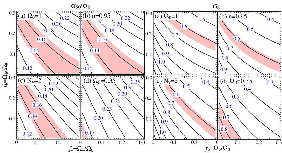
Figure 3: (a–d) Ratio of fluctuations within $50h^{-1}{\rm\,Mpc}$ spheres to that within $8h^{-1}{\rm\,Mpc}$ spheres as a function of neutrino and baryon fractions for various cosmologies. The shaded region shows the preferred range of $\sigma_{50}/\sigma_{8}=0.151\pm 0.016$. (a) $\Omega_{0}=1$, $h=0.5$, $n=1$, $N_{\nu}=1$. (b) As (a), but with $n=0.95$ and tensors as per power-law inflation. (c) As (a), but with two degenerate neutrino species ($N_{\nu}=2$). (d) $\Omega_{0}=0.35$, $\Omega_{\Lambda}=0.65$, $h=0.7$, $n=1$, $N_{\nu}=1$. All are COBE-normalized. (e–h) Amplitude of fluctuations within $8h^{-1}{\rm\,Mpc}$ spheres for the cosmologies given in (a–d), respectively. The shaded region is the preferred range of $\sigma_{8}=(0.5\pm 0.15)\Omega_{0}^{-0.65}$ (Pen  1997) and $\sigma_{8}>0.59$ (Fan et al.  1997).

We begin at large scales and consider the shape of the linear power spectrum as reconstructed from galaxy surveys. Peacock & Dodds (1994) considered a collection of data sets vis-a-vis zero-baryon power spectrum models; they found that scale-invariant models with $\Gamma\equiv\Omega_{0}h=0.255\pm 0.017$ provided the best fit. However, adding baryons and/or neutrinos alters the shape and hence the best fit. We do not perform this detailed reanalysis here; rather we use the ratio of large-scale to small-scale power as a proxy for the shape (see e.g. White et al.  1996). In particular, we construct the ratio of the amplitude of density-weighted fluctuations ($P_{cb\nu}$) within a $50h^{-1}{\rm\,Mpc}$ tophat to those within a $8h^{-1}{\rm\,Mpc}$ tophat, i.e. $\sigma_{50}/\sigma_{8}$. The range $\Gamma=0.25\pm 0.05$, which we conservatively adopt, converts to $\sigma_{50}/\sigma_{8}=0.151\pm 0.016$. Note that high values of $\Gamma$ produce lower values of $\sigma_{50}/\sigma_{8}$.

We display this ratio in Figure 3a–d (left panel) as a function of baryon fraction and neutrino fraction. It is important to note that baryons play as important a role as neutrinos in suppressing power on cluster scales relative to larger scales (White et al.  1996). For example, even the cosmic concordance model (Ostriker & Steinhardt  1995) of $\Omega_{0}=0.35$ with $h=0.7$, which seems to have an appropriate $\Gamma$, stretches the constraint when pushed to the 10–15% baryon fraction suggested by cluster mass determinations (e.g. White et al.  1993b; David et al.  1995; White & Fabian  1995; Evrard  1997).

5.2 Cluster Abundance

The present-day abundance of rich clusters of galaxies is a sensitive probe of mass fluctuations on the $8h^{-1}{\rm\,Mpc}$ scale (Evrard  1989; White et al.  1993a; Eke et al.  1996; Viana & Liddle  1996; Bond & Myers 1996; Pen 1997). We adopt the determination of Pen (1997)

$$\sigma_{8}\approx 0.5\Omega_{0}^{-0.65}$$ (41)

and take a conservative range of 30% errors (i.e. $0.5\pm 0.15$).

The time evolution of the abundance of clusters provides a way to isolate $\sigma_{8}$ from its $\Omega_{0}$ dependence. By comparing the abundance of high-redshift clusters relative to the present-day abundance, Fan et al.  (1997) found $\sigma_{8}=0.83\pm 0.15(1\sigma)$. To be conservative, we employ a $2\sigma$ lower limit (from the relevant quantity, $\sigma_{8}^{-2}$) of $\sigma_{8}>0.59$.

Fig. 3e–h (right panel) shows the cluster abundance constraints for the same 4 models as Fig. 3a–d. As is well-known, high-$\Omega_{0}$ cosmologies with small tilt and trace baryon and neutrino content overproduce present-day clusters. Adding a substantial fraction of baryons or neutrinos makes the models marginally consistent with both the present-day and high-redshift cluster abundances.

5.3 Damped Ly${\boldmath\alpha}$ Systems

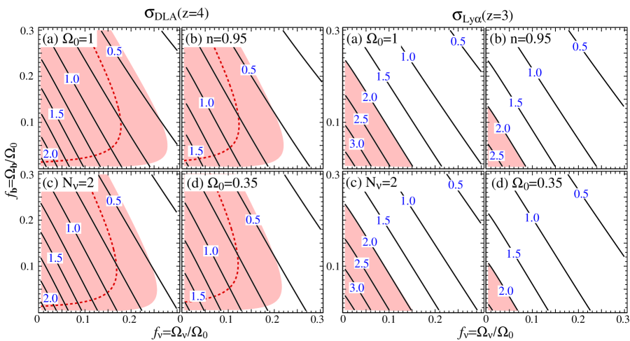
Figure 4: (a–d) Amplitude of fluctuations at $z=4$ within a Gaussian window of mass corresponding to halos of $50{\rm\,km\,\,s^{-1}\,\,Mpc^{-1}}$ circular velocity. Cosmologies are as per Figure 3. The shaded region indicates cosmologies where the neutral gas in halos of $v_{c}>50{\rm\,km\,\,s^{-1}\,\,Mpc^{-1}}$ [using the prescription of Klypin et al.  (1995) and $f_{{\rm H\,\sc i}}=1$] exceeds that observed in damped Ly$\alpha$ systems. The region to the left of the dashed line is the allowed region for $f_{{\rm H\,\sc i}}=0.1$. (e–h) Amplitude of fluctuations at $z=3$ for a Gaussian window of radius $0.0416(\Omega_{0}h^{2})^{-1/2}{\rm\,Mpc}$, suggested by Gnedin (1997) as a indicator of the slope of the column-density distribution of the Ly$\alpha$ forest. The region $\sigma_{{\rm Ly}\alpha}>2$ is shaded. Cosmologies are as in Figure 3.

Cosmologies with moderate neutrino fractions have a strong suppression of power on small scales. This implies that they form proto-galactic systems later than pure-CDM models. Indeed, these models may have trouble forming high-redshift objects such as quasars (e.g. Ma & Bertschinger  1994; Liddle et al.  1996), UV-dropout galaxies (Mo & Fukugita 1996), and damped Ly$\alpha$ systems (Mo & Miralda-Escudé  1994; Ma & Bertschinger  1994; Kauffmann & Charlot  1994; Klypin et al.  1995). We focus on the last of these.

Observations of damped Ly$\alpha$ absorption systems in QSO spectra may be interpreted as a measurement of the mean density of neutral hydrogen $\Omega_{\rm gas}$, in units of the critical density. Recent measurements at $z=4$ (Storrie-Lombardi et al.  1996) find this to be

$$\Omega_{\rm gas}(z\approx 4)=(9.3\pm 3.8)\times 10^{-4}h^{-1}\left[(1+z)^{3/2}g(z)\right]\Big{|}_{z=4}.$$ (42)

Assuming Poisson statistics, we adopt a 95% lower limit of 43% of the central value.

One can estimate an upper limit to the value of $\Omega_{\rm gas}$ in a particular cosmology by assuming that all gas in proto-galactic halos is neutral and using the Press-Schechter formalism (Press & Schechter  1974) to estimate the number of such halos (Mo & Miralda-Escudé  1994; Kauffmann & Charlot  1994; Ma & Bertschinger  1994; Klypin et al.  1995; Liddle et al.  1996). These works differ in their Press-Schechter implementation; here we adopt the conservative assumptions of Klypin et al. (1995). We define $\sigma_{\rm DLA}$ to be the amplitude of fluctuations (using $P_{cb\nu}$) inside a Gaussian window of a scale corresponding to a circular velocity $v_{c}$ of $50{\rm\,km\,\,s^{-1}\,\,Mpc^{-1}}$. The relation between mass and velocity is (Narayan & White  1987)

$$M={v_{c}^{3}\over\sqrt{89}GH_{0}g(z)},$$ (43)

where $g(z)$ is defined in equation (9). Then the density of neutral gas arising from all halos with velocities greater than $50{\rm\,km\,\,s^{-1}\,\,Mpc^{-1}}$ is

$$\Omega_{\rm gas}=f_{{\rm H\,\sc i}}\Omega_{b}\,{\rm erfc}\left(\delta_{c}\over\sqrt{2}\sigma_{\rm DLA}\right),\qquad f_{{\rm H\,\sc i}}\leq 1$$ (44)

where $f_{{\rm H\,\sc i}}$ is the fraction of neutral gas, erfc($x$) is the complimentary error function, and we take a density threshold of $\delta_{c}=1.33$.

In Figure 4a–d (left panel), we plot $\sigma_{\rm DLA}$ as a function of cosmological parameters. We superpose the constraint implied by comparing equation (42) to equation (44) with $f_{{\rm H\,\sc i}}=1$. As found by previous studies, MDM models with $f_{\nu}\gtrsim 0.3$ underproduce high-redshift halos; the constraints are tighter for higher $f_{b}$, red-tilted, and degenerate-neutrino models. The limits in Figure 4 are actually extremely conservative; hydrodynamical studies (Ma et al.  1997; Gardner et al.  1997a,b) infer $f_{{\rm H\,\sc i}}\lesssim 0.1$ in tested cases. Correspondingly, we plot the limits if $f_{{\rm H\,\sc i}}=0.1$ in dashed lines to show how this uncertainty affects the cosmological constraints. Since it is difficult to scale these numerical corrections as functions of cosmological parameters, especially if varying $\Omega_{b}$ (Gardner et al.  1997b), the $f_{{\rm H\,\sc i}}=0.1$ line should not be taken as a firm constraint.

5.4 Ly${\boldmath\alpha}$ Forest

If the low column density absorption features in QSO spectra arise from mild density and velocity perturbations in the IGM (Cen et al.  1994; Petijean et al.  1995; Zhang et al.  1995, 1997; Miralda-Escudé et al.  1996; Hernquist et al.  1996), then the correlations and column-density distribution of the lines may yield robust information about the power spectrum on sub-Mpc scales. Croft et al.  (1997) demonstrated that the power spectrum of simulations could be reconstructed from absorption spectra drawn from them. Gnedin  (1997) showed that the power-law exponent of the column density distribution in various cosmological simulations is strongly correlated with the amplitude of linear fluctuations on the smallest collapsing scales. Comparing to the observed distribution suggests a lower bound on the amplitude of fluctuations on mass scales near $10^{9}{\rm\,M_{\odot}}$ at $z=3$. In particular, the quantity $\sigma_{{\rm Ly}\alpha}$, defined as the fluctuations inside a Gaussian window of radius $R=0.0416(\Omega_{0}h^{2})^{-1/2}{\rm\,Mpc}$ using $P_{cb}$, is constrained to be greater than 2.0 at $z=3$. The scale is chosen to approximate the Jeans length at $z=3$ for common thermal histories (Gnedin  1997). This constraint is plotted in Figure 4e–h (right panel).

5.5 Summary

Even in the standard COBE-normalized, $n=1$, $\Omega_{0}=1$ model, the inclusion of a moderate fraction of baryons or neutrinos can decrease $\sigma_{8}$ to an appropriate level. Models that accomplish this by the neutrino fraction alone produce insufficient power to explain damped Ly$\alpha$ absorption systems. Models that accomplish this by the baryon fraction alone require baryon densities far in excess of big bang nucleosynthesis predictions. Although a compromise of $\Omega_{b}=0.15$ and $\Omega_{\nu}=0.25$ would work, Figure 3 shows that no model in this scenario fits the $\sigma_{50}/\sigma_{8}$ and $\sigma_{8}$ constraints.

However, the modest change of altering the tilt to 0.95 (with tensors) or adding a second degenerate neutrino species opens regions of parameter space that match both large-scale structure and constraints from damped Ly$\alpha$ systems. For example, models with $\Omega_{b}=0.1$, $h=0.5$, and either $\Omega_{\nu}=0.15$ with $n=0.95$ or $\Omega_{\nu}=0.2$ with $N_{\nu}=2$ produce $\sigma_{8}\approx 0.64$ and match the high-redshift constraints with $f_{{\rm H\,\sc i}}\sim 0.2$. $f_{{\rm H\,\sc i}}\approx 0.1$ could be achieved by reducing the COBE normalization by 7% (a $1-\sigma$ shift) and decreasing $\Omega_{\nu}$ so as to keep $\sigma_{8}$ constant. The higher value of $\Omega_{b}$—as compared to the canonical value of 0.05 from Walker et al.  (1991) but in agreement with Tytler et al.  (1996)—is doubly useful in meeting the requirements: the suppression due to baryons occurs at larger scales than that from neutrinos and therefore alters $\sigma_{8}$ more effectively, while the additional baryons are available to produce high-redshift absorption. Moreover, this value of $\Omega_{b}$ better agrees with the baryon fraction in clusters (e.g. White et al.  1993b; David et al.  1995; White & Fabian  1995; Evrard  1997) and that inferred from the Ly$\alpha$ forest (e.g. Miralda-Escudé et al.  1996; Weinberg et al.  1997; Zhang et al.  1997).

The more common solution to the problems of $\Omega_{0}=1$ CDM is to reduce the value of $\Omega_{0}$ to around $0.3$. As shown in Figures 3 and 4, this satisfies the quoted constraints when used with small baryon and neutrino fractions. An important lesson of the figures, however, is that small admixtures of baryons or neutrinos can make significant changes. For example, the $\Omega_{0}=0.35$ flat model presented here tends to underproduce power even with only a 10% baryon fraction ($\Omega_{b}h^{2}=0.017$). The lack of small-scale power in such models places more stringent limits on $\Omega_{\nu}/\Omega_{0}$ than in high-density cosmologies; this implies a stronger limit for the neutrino mass $m_{\nu}\propto\Omega_{\nu}h^{2}$. Of course, a small blue tilt would help the situation.

It is very interesting to note that early results from modeling the Ly$\alpha$ forest (§5.4, Fig. 4e–h) are more effective at excluding models than constraints from damped systems. The limits suggested by Gnedin  (1997) would eliminate all of the $\Omega_{0}=1$ models studied in Figures 3 and 4. Perhaps models with blue tilts ($n>1$) would succeed in producing sufficient amounts of small-scale power, although of course they would require more suppression of power at cluster scales relative to COBE. Constraints from the Ly$\alpha$ forest are still only preliminary, but they appear to be quite promising.

6 Conclusion

In this paper, we have considered adiabatic models composed of baryons, cold dark matter, and massive neutrinos. We have presented a fitting formula for the linear transfer function of such models, including the possibility of $\Omega_{0}\neq 1$ and multiple degenerate neutrino models. The parameter space covered by the formula is much larger than that previously available; we provide functions of space, time, and six cosmological parameters. The accuracy is $\lesssim 5\%$ in the central range of $0.06\lesssim\Omega_{0}h^{2}\lesssim 0.40$, $\Omega_{b}/\Omega_{0}\leq 0.3$, $\Omega_{\nu}/\Omega_{0}\leq 0.3$, and $z<30$ and improves to $\lesssim 3\%$ for models with baryon fractions below 10%.

An accurate, general fitting formula allows one to calculate statistics of the power spectrum as functions of cosmological parameters quite efficiently. As an example of this, we presented several different observational tests and displayed the constraints as functions of baryon fraction and neutrino fraction for various choices of the other cosmological parameters. Baryons and neutrinos are both effective at suppressing small-scale power relative to that on larger scales. We find that models with large baryon fractions are less “observationally-challenged”, in that a given reduction on cluster scales (i.e. $\sigma_{8}$) imposes less suppression on very small scales, where power is needed to produce damped Ly$\alpha$ systems and other high-redshift objects. Hence, if $\Omega_{b}$ is as large as 0.1, as suggested by Tytler et al.  (1996) for $h=0.5$, then constraints on mixed dark matter models are weakened. For example, with a tilt of $n=0.95$, an MDM model with $\Omega_{\nu}=0.15$ and $\Omega_{b}=0.1$ fares significantly better than one with $\Omega_{\nu}=0.2$ and $\Omega_{b}=0.05$. Finally, we find that the constraint on the small-scale power as derived from the slope of the column-density distribution of the Ly$\alpha$ forest (Gnedin  1997) is an extremely powerful limit on MDM models. Further work is needed to test the robustness of this inference.

The observations discussed above place constraints upon the neutrino mass, although these limits vary with other presently unknown parameters, e.g. $\Omega_{0}$, $h$, $\Omega_{b}$, and $n$. Future CMB observations should precisely determine these quantities (Jungman et al.  1996; Bond et al.  1997; Zaldarriaga et al.  1997) but will have little leverage on $\Omega_{\nu}$ (Ma & Bertschinger 1995; Dodelson et al.  1996a). However, the combination of CMB data with large-scale structure observations will allow a robust determination of $\Omega_{\nu}$. Further observations and modeling of damped Ly$\alpha$ systems and the Ly$\alpha$ forest will corroborate this but may not be clean enough to yield a precise measurement. If $\Omega_{0}$ is found to be low, our sensitivity to the neutrino mass will be stronger because the suppression of small-scale power depends on $\Omega_{\nu}/\Omega_{0}$; this differs from the trend in the CMB, where lowering $\Omega_{0}$ shifts the effects of neutrinos to smaller angular scales. This illustrates the power of combining cosmological data sets with regard to determining the properties of the dark matter.

The formulae in §3 of this paper are available in electronic form at

http://www.sns.ias.edu/$\sim$whu/transfer/transfer.html.

We also include a driver that calculates COBE-normalized $\sigma_{8}$ and other constraints from §5 as a function of cosmological input parameters.

Acknowledgments: We thank D. Spergel and M. White for useful discussions. D.J.E. and W.H. are supported by NSF PHY-9513835. W.H. was additionally supported by the W.M. Keck Foundation. Numerical results were taken from the CMBfast package of Seljak & Zaldarriaga (1996).

References

- (1) Achilli, S., Occhionero, F., & Scaramella, R. 1985, ApJ, 299, 577
- (2) Bardeen, J.M., Bond, J.R., Kaiser, N. & Szalay, A.S. 1986, ApJ, 304, 15
- (3) Bildhauer, S., Buchert, T., & Kasai, M. 1992, A&A, 263, 23
- (4) Bond, J.R., & Efstathiou, G. 1984, ApJ, 285, L45
- (5) Bond, J.R., Efstathiou, G., & Silk, J. 1980, Phys. Rev. Lett., 45, 1980
- (6) Bond, J.R., & Szalay, A. 1983, ApJ, 276, 443
- (7) Bond, J.R. & Myers, S.T. 1996, ApJS, 103, 63
- (8) Bond, J.R., Efstathiou, G., Tegmark, M. 1997, MNRAS, in press [astro-ph/9702100]
- (9) Bunn, E.F., & White, M. 1997, ApJ, 480, 6
- (10) Carroll, S.M., Press, W.H., Turner, E.L. 1992, ARA&A, 30, 499
- (11) Cen, R., Gnedin, N.Y., Kofman, L.A., Ostriker, J.P. 1992, ApJ, 399, L11
- (12) Cen, R., Miralda-Escudé, J., Ostriker, J.P., & Rauch, M. 1994, ApJ, 437, L9
- (13) Croft, R.A.C., Weinberg, D.H., Katz, N., & Hernquist, L. 1997, ApJ, submitted [astro-ph/9708018]
- (14) David, L.P., Jones, C., & Forman, W. 1995, ApJ, 445, 578
- (15) Davis, M., Summers, F., & Schlegel, D. 1992, Nature, 359, 393
- (16) Dodelson, S., Gates, E., & Stebbins, A. 1996a, ApJ, 467, 10
- (17) Dodelson, S., Gates, E., & Turner, M.S. 1996b, Science, 274, 69 [astro-ph/9603081]
- (18) Edwards, D., & Heath, D. 1976, Ap Space Sci, 41, 183
- (19) Efstathiou, G., Bond, J.R., & White, S.D.M. 1992, MNRAS, 258, P1
- EH (97) Eisenstein, D.J. & Hu, W. 1997, ApJ, submitted [astro-ph/9709112] (EH97)
- (21) Eke, V.R., Cole, S., & Frenk, C.S. 1996, MNRAS, 282, 263
- (22) Evrard, A.E. 1989, ApJ, 341, L71
- (23) Evrard, A.E. 1997, MNRAS, submitted [astro-ph/9701148]
- (24) Fang, L.Z., Li, S.X., Xiang, S.P. 1984, A&A, 140, 77
- (25) Fan, X., Bahcall, N., Cen, R. 1997, ApJL, submitted [astro-ph/9709265]
- (26) Fixsen, D. et al. 1996, ApJ, 473, 576 [astro-ph/9605054]
- (27) Gardner, J.P., Katz, N., Weinberg, D.H., Hernquist, L. 1997, ApJ, 484, 31
- (28) Gardner, J.P., Katz, N., Weinberg, D.H., Hernquist, L. 1997, ApJ, 486, 42
- (29) Gnedin, N.Y. 1997, MNRAS, submitted [astro-ph/9706286]
- (30) Groth, E.J. & Peebles, P.J.E. 1975, A&A, 41, 143
- (31) Heath, D.J. 1977, MNRAS, 179, 351
- (32) Hernquist, L., Katz, N., Weinberg, D.H., & Miralda-Escudé, J. 1996, ApJ, 457, L51
- (33) Holtzman, J.A. 1989, ApJS, 71, 1
- (34) Holtzman, J.A., & Primack, J.R. 1993, ApJ, 405, 428
- HE (97) Hu, W., & Eisenstein, D.J. 1997, ApJ, submitted [astro-ph/9710216] (HE97)
- (36) Hu, W. & Sugiyama, N. 1996, ApJ, 471, 542 (HS96) [astro-ph/9510117]
- (37) Hu, W., & White, M. 1997, ApJ, 486, L1 [astro-ph/9701210]
- (38) Jungman, G., Kamionkowski, M., Kosowsky, A., Spergel, D.N. 1996, Phys. Rev. D, 54, 1332
- (39) Kauffmann, G. & Charlot, S. 1994, ApJ, 430, L97 [astro-ph/9402015]
- (40) Klypin, A., Holtzman, J., Primack, J., & Regös, E. 1995, ApJ, 416, 1
- (41) Klypin, A. Borgani, S., Holtzman, J.A., Primack, J.R. 1995, ApJ, 441, 1 [astro-ph/9407011]
- (42) Kolb, E.W., & Turner, M.S. 1990, The Early Universe (Redwood City, CA: Addison-Wesley)
- (43) Lahav, O., Rees, M.J., Lilje, P.B., & Primack, J.R. 1991, MNRAS, 251, 128
- (44) Liddle, A. et al. 1996, MNRAS, 281, 531 [astro-ph/9511057]
- (45) Ma, C.-P. 1996, ApJ, 471, 13 [astro-ph/9605198]
- (46) Ma, C.-P. & Bertschinger, E. 1994, ApJ, 434, L5
- (47) Ma, C.-P. & Bertschinger, E. 1995, ApJ, 455, 7 [astro-ph/9506072]
- (48) Ma, C.-P., Bertschinger, E., Hernquist, L., Weinberg, D.H. & Katz, N. 1997, ApJ, 484 L1 [astro-ph/9705113]
- (49) Miralda-Escudé, J., Cen, R., Ostriker, J.P., & Rauch, M. 1996, ApJ, 471, 582
- (50) Mo, H.J. & Fukugita, M. 1996, ApJ, L9 [astro-ph/9604034]
- (51) Mo, H.J. & Miralda-Escudé, J. 1994, ApJ, 430, L25 [astro-ph/9402014]
- (52) Narayan, R., & White, S.D.M. 1987, MNRAS, 231, 97p
- (53) Ostriker, J.P. 1993, ARA&A, 31, 689
- (54) Ostriker, J.P., & Steinhardt, P.J. 1995, Nature, 377, 600 [astro-ph/9505066]
- (55) Peacock, J.A., & Dodds, S.J. 1994, MNRAS, 267, 1020
- (56) Peebles, P.J.E. 1980, Large-Scale Structure of the Universe (Princeton: Princeton Univ. Press)
- (57) Peebles, P.J.E. 1993, Principles of Physical Cosmology (Princeton: Princeton Univ. Press), §25
- (58) Pen, U.-L. 1997, preprint [astro-ph/9610147]
- (59) Petijean, P., Mücket, J.P., & Kates, R. 1995, A&A, 295, L9
- (60) Pogosyan, D. Yu., & Starobinsky, A.A. 1995, MNRAS, 447, 465
- (61) Press, W.H. & Schechter, P.L. 1974, ApJ, 197, 425
- (62) Primack, J.R., Holtzman, J., Klypin, A., & Caldwell, D.0. 1995, Phys. Rev. Lett., 74, 2160 [astro-ph/9411020]
- (63) Seljak, U. & Zaldarriaga, M. 1996, ApJ, 469, 437 [astro-ph/9603033]
- (64) Schaefer, R.K. & Shafi, Q. 1992, Nature, 358, 199
- (65) Storrie-Lombardi, L.J., Irwin, M.J., & McMahon, R.G. 1996, MNRAS, 283, L79 [astro-ph/9608146]
- (66) Taylor, A.N. & Rowan-Robinson, M. 1992, Nature, 359, 396
- (67) Tytler, D., Fan, X.M., & Burles, S. 1996, Nature, 381, 207 [astro-ph/9603069]
- (68) Valdarnini, R., & Bonometto, S.A. 1985, A&A, 146, 235
- (69) Viana, P.T.P. & Liddle, A.R. 1996, MNRAS, 281, 323
- (70) Walker, T.P., Steigman, G., Kang, H., Schramm, D.M., Olive, K.A. 1991, ApJ, 376, 51
- (71) Weinberg, S. 1972, Gravitation and Cosmology (New York: Wiley)
- (72) Weinberg, D.H., Miralda-Escudé, J., Hernquist, L., & Katz, N. 1997, ApJ, submitted [astro-ph/9701012]
- (73) White, D.A., & Fabian, A.C. 1995, MNRAS, 273, 72
- (74) White, M., Viana, P., Liddle, A., & Lyth, D. 1996, MNRAS, 283, 107 [astro-ph/9605057]
- (75) White, S.D.M., Efstathiou, G., & Frenk, C.S. 1993, MNRAS, 262, 1023
- (76) White, S.D.M., Navarro, J.F., Evrard, A.E., & Frenk, C.S. 1993, Nature, 366, 429
- (77) Yamamoto, K., Sugiyama, N., & Sato, H. 1997, ApJ, submitted [astro-ph/9709247]
- (78) Zaldarriaga, M., Spergel, D.N., & Seljak, U. 1997, ApJ, 488, 1 [astro-ph/9702157]
- (79) Zhang, Y., Anninos, P., & Norman, M.L. 1995, ApJ, 453, L57
- (80) Zhang, Y., Meiksin, A., Anninos, P., & Norman, M.L. 1997, ApJ, in press [astro-ph/9706087]