The Hot Galactic Corona and the Soft X-ray Background

Abstract

I characterize the global distribution of the 3/4 keV band background with a simple model of the hot Galactic corona, plus an isotropic extragalactic background. The corona is assumed to be approximately polytropic (index = 5/3) and hydrostatic in the gravitational potential of the Galaxy. The model accounts for X-ray absorption, and is constrained iteratively with the ROSAT all-sky X-ray survey data. Regions where the data deviate significantly from the model represent predominantly the Galactic disk and individual nearby hot superbubbles. The global distribution of the background, outside these regions, is well characterized by the model; the $1\sigma$ relative dispersion of the data from the model is $\sim 15\%$. The electron density and temperature of the corona near the Sun are $\sim 1.1\times 10^{-3}{\rm~{}cm^{-3}}$ and $\sim 1.7\times 10^{6}$ K. The same model also explains well the 1.5 keV band background. The model prediction in the 1/4 keV band, though largely uncertain, qualitatively shows large intensity and spectral variations of the corona contribution across the sky.

1 Introduction

Although Spitzer (1956) speculated the presence of a hot ($\sim 10^{6}$ K) Galactic corona around the Milky Way more than 40 years ago, direct observational evidence of it comes only recently. The very existence of hot gas far away from the Sun is shown convincingly first by the the detection of the shadow cast by the Draco cloud ($D\lower 2.0pt\hbox{$\,\buildrel\scriptstyle>\over{\scriptstyle\sim}\,$}300$ pc; $z\lower 2.0pt\hbox{$\,\buildrel\scriptstyle>\over{\scriptstyle\sim}\,$}200$ pc) against the 1/4 keV background (Burrows & Mendenhall 1991; Snowden et al. 1991). Based on the X-ray shadowing of the Magellanic Bridge ($D\sim 60$ kpc), Wang & Ye (1996) further find that $\sim 30\%$ of the background observed at $\sim 0.7$ keV is Galactic in origin. At this energy, however, the contribution from the Local Hot Bubble around the Sun appears negligible (Snowden, McCammon, & Verter 1993; Kuntz, Snowden, & Verter 1997), although the Bubble is responsible for most of the background in the 1/4 keV band (e.g., Snowden et al. 1997a). Moreover, the ROSAT all-sky survey (Snowden et al. 1995; 1997b) clearly shows an overall intensity enhancement in the 0.5-2 keV range over the Galactic center hemisphere. Snowden et al. have suggested that this enhancement may represent a bulge of hot gas around the Galactic center.

I have tested how a simple, physically self-consistent model of the hot Galactic corona may account for the soft X-ray background, especially in the 3/4 keV band. The radiation in this band is sensitive to gas at temperatures $\lower 2.0pt\hbox{$\,\buildrel\scriptstyle>\over{\scriptstyle\sim}\,$}1.5\times 10^{6}$ K and is not as heavily attenuated by the X-ray-absorbing interstellar medium as in the 1/4 keV band. Furthermore, the effect of the small-scale ($\lower 2.0pt\hbox{$\,\buildrel\scriptstyle<\over{\scriptstyle\sim}\,$}1^{\circ}$) clumpiness of the medium may be negligible over a unit X-ray absorption depth of $\sim 2\times 10^{21}{\rm~{}cm^{-2}}$. It is clear, though, that the observed background is strongly contaminated by various discrete X-ray sources in regions near the Galactic plane and by a few high Galactic latitude features such as Loop I and Eridanus superbubbles. I have therefore devised data reduction and analysis algorithms to minimize the effects of these contaminations. The results are encouraging. The model provides a frame work for both characterizing the global hot gas distribution of the Galactic corona and defining discrete X-ray-emitting features.

In the following, I first talk about the data analysis and modeling procedures, and then present some preliminary results. Finally, I make some comparisons of the results with other independent measurements and extend the results into the 1/4 keV and 1.5 keV bands.

2 Data Analysis

The data used in this analysis come from the all-sky surveys made with ROSAT (e.g., Snowden et al. 1995) and IRAS (e.g., Boulanger & Perault 1988). The ROSAT data, in three energy bands ($\sim 1/4$ keV, 3/4 keV, 1.5 keV), were down-loaded from MPE (http://www.rosat.mpe-garching.mpg.de/), and the IRAS 100$\mu$m data from HEASARC (http://skview.gsfc.nasa.gov/). The data were presented as surface brightness intensity maps (480$\times$240 pixels), Aitoff-projected in the Galactic coordinates. These maps, though not reflecting the intrinsic spatial resolutions (a few arcminutes) of the surveys, provide a convenient database for investigating the global distributions of both the X-ray background and the X-ray-absorbing medium.

For my data modeling purpose, I processed the data in three major steps. First, to approximately correct for the zero intensity level of the IRAS data, I shifted the 100$\mu$m map to match the estimated total absorption $9\times 10^{19}{\rm~{}cm^{-2}}$ in the Lockman Hole region (Snowden et al. 1994), using a conversion of 1.14 $\times 10^{20}{\rm~{}cm^{-2}/(MJy~{}sr^{-1}})$ (Boulanger & Perault 1988; Snowden et al. 1997a). Second, I removed strips of pixels that were not, or very poorly, covered in the surveys. Third, I compressed the maps by taking a median summary in each non-overlapping square of 3$\times$3 pixels. I discarded any square that contained one or more removed pixels (including those outside the sky projection). The median summary, as a resistant statistic, effectively removed the effects of outstanding small-scale ($\lower 2.0pt\hbox{$\,\buildrel\scriptstyle<\over{\scriptstyle\sim}\,$}1$ deg) features (e.g., nearby galaxies and AGNs). The top panels of Fig. 1 present the processed data.

3 Modeling

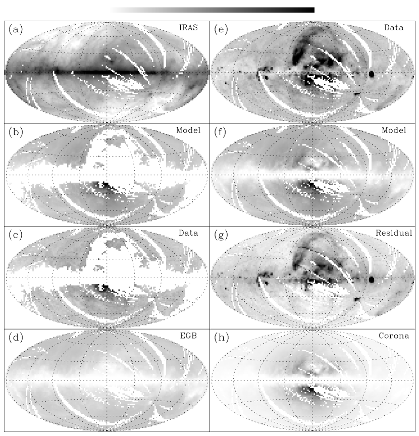
Figure 1: Surface brightness intensity maps in the zero-centered Galactic coordinates with Aitoff equal-area projections. Both X-ray data and model are in the 3/4 keV band. From the top panel to the bottom one in the left column are the zero-level corrected IRAS 100$\mu$m survey (a); Model map covering only pixels used in the fit at the threshold 0.4 (b); ROSAT data in the same region (c); and the extragalactic background component of the model (d). The panels in the right column, arranged for an easy comparison with Fig. 4, are the ROSAT data (e); the model including regions not used in the fit (f); the residual of the ROSAT survey minus the model (g); the corona component of the model (h). The false color range is between 1 and $440{\rm~{}MJy~{}sr^{-1}}$ logrithmetically for (a), 0 to 5 $\times 10^{-4}{\rm~{}counts~{}s^{-1}~{}arcmin^{-2}}$ linearly for (b), (c), (d), (e), (f), and (h), and -0.7 to 5 $\times 10^{-4}{\rm~{}counts~{}s^{-1}~{}arcmin^{-2}}$ for (g); the black represents the lowest intensity while the yellow is the highest. (Referee: The color version of this figure can be found at http://www.astro.nwu.edu/astro/wqd/paper/halo/)

To capture the global distribution of the X-ray background, I have considered a model that consists of two contributions: an isotropic extragalactic background (EGB) and an axisymmetric Galactic corona. The corona is assumed to be quasi-hydrostatic in the gravitational potential of the Galaxy (Wolfire et al. 1995; Johnston, Spergel, & Hernquist 1995). The potential is a sum of three components: a Miyamoto-Nagai disk, a spheroid bulge, and a logarithmic halo. These components together provide a nearly flat rotation curve from 1 to 30 kpc with a circular velocity of $225{\rm~{}km~{}s^{-1}}$ at the Galacto-centric radius 8.5 kpc of the Sun. It is the disk component, however, that is chiefly responsible for the corona structure visible in the ROSAT band. For ease of modeling, I neglect the angular momentum of the corona. The momentum should be small if the corona is fueled primarily by hot gas from the Galactic central region. Observations of nearby disk galaxies do indicate that hot gas outflows happen primarily in galactic center regions (e.g., Wang et al. 1995; Pietch, Supper, & Vogler 1995). Furthermore, because the cooling of the hot gas at temperatures $\lower 2.0pt\hbox{$\,\buildrel\scriptstyle>\over{\scriptstyle\sim}\,$}10^{6}$ K is most likely adiabatic, a polytropic equation of state of index 5/3 may be a reasonably good description of the hot gas. The shape and normalization of this model corona are determined by two adjustable parameters, chosen here to be the electron density ($n_{o}$) and temperature ($T_{o}$) of the corona near the Sun.

I calculate a model X-ray background, accounting for both the X-ray absorption and the ROSAT/PSPC spectral response. The calculation makes the following assumptions: (1) The EGB has a spectrum characterized by a power law of energy slope equal to 1 (e.g., Hasinger et al. 1993); (2) The hot gas of the corona is in a collisional ionization equilibrium (Raymond & Smith 1977); (3) Both the hot gas and the X-ray-absorbing medium are of solar metal abundances; (4) The absorption is foreground, which should be reasonably good except for regions close to the Galactic plane ($|b|\lower 2.0pt\hbox{$\,\buildrel\scriptstyle<\over{\scriptstyle\sim}\,$}10^{\circ}$). X-ray surface brightness intensities of a unit volume are calculated first in a grid as a function of hot gas temperature and X-ray-absorbing medium column density. Based on this grid, an intensity integration along a line of sight can be carried out efficiently. The integrated intensity of the corona, together with a partially absorbed EGB contribution, constitutes the model intensity $m_{i}$, where $i$ represents a line of sight, or a pixel in a background map (Fig. 1).

The intrinsic intensity $I_{e}$ of the EGB as well as the corona parameters, $n_{o}$ and $T_{o}$, are constrained by a model fit to the ROSAT survey data $d_{i}$ in the 3/4 keV band. Specifically, the fit minimizes the statistic $\chi^{2}=\sum[(d_{i}-m_{i})w_{i}]^{2}$, where the summation is over the adopted map pixels. The weight $w_{i}$ is inversely proportional to the pixel-to-pixel intensity dispersion, $\sim 15\%m_{i}$, estimated in regions away from local X-ray enhancements (see also §4). In comparison, the counting statistical uncertainty is considerably smaller ($\lower 2.0pt\hbox{$\,\buildrel\scriptstyle<\over{\scriptstyle\sim}\,$}5\%$) in a $\sim 4~{}{\rm deg}^{2}$ pixel with a typical exposure $\sim 500$ s of the ROSAT survey. Adding this uncertainty in the weight would cause only minor ($\lower 2.0pt\hbox{$\,\buildrel\scriptstyle<\over{\scriptstyle\sim}\,$}5\%$) changes in the results. The fit is conducted iteratively to remove outliers — pixels where the data deviate significantly from the model. Starting with $w_{i}=$ constant, the fit gets an initial estimate of the model $m_{i}$. $w_{i}$ is then recalculated. After removing those pixels with relative deviations $(d_{i}-m_{i})w_{i}>2$, an arbitrarily chosen initial threshold, the fit proceeds to minimize $\chi^{2}$ again and so on, until no more pixel has $(d_{i}-m_{i})w_{i}>2$. Next, the threshold is reduced by 10%, an arbitrarily chosen step, and a new round of fitting and pixel removing starts. Fig. 2 shows how the model parameter fits evolve with the deviation threshold for pixel-removing. When the threshold is large, the outliers strongly influence the fit of the parameters, especially $n_{o}$ and $I_{e}$. The parameter values also fluctuate until the threshold is reduced to $\sim 0.2$, when nearly half of the map pixels are removed. The results are not particularly sensitive to either the initial threshold or the step.

Figure 2: Parameter changes with the pixel-removing threshold. The model fitting proceeds from the right to the left.

4 Results

Fig 1 includes a comparison of the data with the model background fitted at the threshold equal to 0.4, at which the parameter values are close to the converging values at $\lower 2.0pt\hbox{$\,\buildrel\scriptstyle<\over{\scriptstyle\sim}\,$}0.2$ and only a quarter of the pixels are removed. While the model is intrinsically symmetric relative to the Galaxy rotation axis, the asymmetric appearance of the model background in Fig. 1 (e.g., Panel f) is due to the foreground X-ray absorption (a). The dispersion of the data from the model is $\sim 0.15\%$, averaged over the pixels remained in the fit (Panels b and c in Fig. 1). Pixels excluded from the fit are almost entirely at the Galactic plane and in high Galactic latitude regions that are contaminated by Loop I (including the Sco-Cen starforming region) and Eridanus superbubbles as well as the Large Magellanic Cloud near the south Elliptical pole (see Snowden et al. 1995 for a graphic illustration). These features and the disk component stand out in the residual map, because of the removal of global emission and absorption effects of the corona and EGB contributions. Part of the residual emission near the Galactic plane, however, may result from an incomplete removal of the corona contribution. The foreground assumption of the X-ray-absorbing medium leads to a slight overestimation of the absorption near the Galactic plane, where some of the medium is located behind the corona emission. While the corona contribution (h) is strongly concentrated in the Galactic center hemisphere, the EGB (d) is more uniformly distributed in the sky, except for regions close to the Galactic plane.

Since the model describes the global distribution of the 3/4 keV background reasonably well, it is tempting to use the model fit as a characterization of the hot Galactic corona. From Fig. 2, I estimate the local hot gas electron density and temperature of the corona as $\sim 1.1\times 10^{-3}{\rm~{}cm^{-3}}$ and $\sim 1.7\times 10^{6}$ K. The uncertainties in these two parameters are $\sim 10\%$, corresponding to the fluctuations of the parameter values in the threshold range of $\lower 2.0pt\hbox{$\,\buildrel\scriptstyle<\over{\scriptstyle\sim}\,$}0.5$. Fig. 3 shows the spatial distribution of hot gas temperature in the corona. The density and temperature at the Galactic center are $\sim 1.2\times 10^{-2}{\rm~{}cm^{-3}}$ and $\sim 8.5\times 10^{6}$ K. The integrated mass, thermal energy, and bolometric luminosity of gas at temperatures $>10^{6}$ K are $3\times 10^{7}M_{\odot}$, $\sim 2\times 10^{56}$ ergs, and $\sim 2\times 10^{40}{\rm~{}ergs~{}s^{-1}}$ (only 15% in the 0.5-2 keV range), respectively. The inferred mean radiative cooling timescale of the gas is then $\sim 3\times 10^{8}$ years. The radiative cooling accounts for about 2% of the total mechanical energy input from supernovae in the Galaxy (assuming one supernova per 30 years and $10^{51}{\rm~{}ergs}$ per supernova).

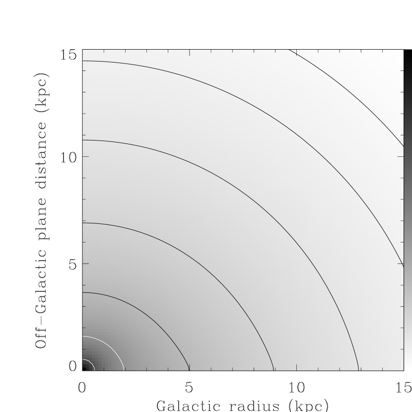
Figure 3: Model gas temperature distribution of the corona in the Galactic cylindrical coordinates. The gray-scale is in the range of 0.18 to 8.4 $\times 10^{6}$ K, while the contours are at 0.5, 0.75, 1.1, 1.7, 2.5, 3.8, and 5.7 $\times 10^{6}$ K.

5 Discussion

The above corona model, constrained by the spatial distribution of the 3/4 keV band background, makes specific predictions that can be compared with various independent measurements. First, the model predicts a thermal pressure of the corona near the Sun as $P/k\sim 3.6\times 10^{3}{\rm~{}K~{}cm^{-3}}$. This prediction is within the uncertainty range of $\sim 2\times 10^{3}-4\times 10^{3}{\rm~{}K~{}cm^{-3}}$ inferred from CIV emission/absorption lines (Martin & Bowyer 1990; Shull & Slavin 1994) and from the two-phase structure of high-velocity clouds (Wolfire et al. 1995). Second, Fig. 3 shows that the spectral characteristics of coronal gas varies strongly in the sky. Based on broad-band spectral properties of the soft X-ray background, various attempts have been made to estimate the average temperature of hot gas beyond the Local Bubble (e.g., Garmire et al. 1992; Wang & McCray 1993; Kerp 1994; Sidher et al. 1996; Snowden et al. 1997b). Such an estimate depends on an assumption about the EGB spectrum, which remains poorly constrained in the 0.1-2 keV range. Nevertheless, the estimated hot gas temperature falls within a range between $\sim 10^{6.0}$ K and $\sim 10^{6.4}$ K. This range can in principle be reproduced with the model, depending on specific lines of sight (Fig. 3). Third, the model predicts a corona contribution of $\sim 3\times 10^{-5}{\rm~{}counts~{}s^{-1}~{}arcmin^{-2}}$ in the PSPC R4 band, which is centered around $0.7$ keV (Snowden et al. 1997b), toward the X-ray shadowing cloud ($l,b=295^{\circ},-42^{\circ}$) in the Magellanic Bridge. This contribution is consistent with the measured Galactic component of $2.7(1.5-3.7)\times 10^{-5}{\rm~{}counts~{}s^{-1}~{}arcmin^{-2}}$ (90% confidence interval; Wang & Ye 1996). Thus the corona model is useful for a uniform explanation of various observations of distant hot gas at high Galactic latitudes.

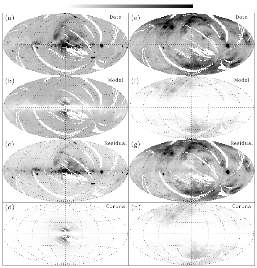
Figure 4: Data and model predictions in the 1.5 keV band (left column) and in the 1/4 keV band (right column). The projections and sky coverage are the same as those in Fig. 1. From the top row to the bottom one are the ROSAT survey data, the model predictions of the corona plus the extragalactic background, the residual maps of the survey data minus the model, and the corona components of the model in the two bands. The false color range in the left column spans between 0 to 5 $\times 10^{-4}{\rm~{}counts~{}s^{-1}~{}arcmin^{-2}}$ for the panels (a), (b) and (d) and -0.7 to 5 $\times 10^{-4}{\rm~{}counts~{}s^{-1}~{}arcmin^{-2}}$ for (c); the range in the right column is all between 0 to 15 $\times 10^{-4}{\rm~{}counts~{}s^{-1}~{}arcmin^{-2}}$. (Referee: The color version of this figure can be found at http://www.astro.nwu.edu/astro/wqd/paper/halo/)

Fig. 4 further compares the model predictions in the 1.5 keV and 1/4 keV bands with the corresponding ROSAT survey data. The data in these bands are processed in the same way as in the 3/4 keV band (§2). The intrinsic EGB intensity is fixed as 1.4 $\times 10^{-4}{\rm~{}counts~{}s^{-1}~{}arcmin^{-2}}$ in the 1.5 keV band, accounting for the total background observed in high Galactic latitude, anti-Galactic center hemisphere, and as 4.2 $\times 10^{-4}{\rm~{}counts~{}s^{-1}~{}arcmin^{-2}}$ in the 1/4 keV band (Barber, Roberts, & Warwick 1996). The model explains well the global distribution of the background in 1.5 keV band. Residual features (Panel c) morphologically mimic those in the 3/4 keV band. The corona contribution is confined more into the central region of the Galaxy than in the 3/4 keV band.

In the 1/4 keV band, the model demonstrates that the corona contribution may vary significantly across the sky in both intensity and spectrum. The model predicts that up to $\sim 45\%$ of the observed background intensity may arise in the corona, depending on individual lines of sight. In the direction of the Draco cloud ($l,b\sim 90^{\circ},39^{\circ}$), for example, the corona contribution is about 30%, which is significantly less than the distant component ($\sim 60\%$) inferred from the X-ray shadowing measurement (e.g., Burrows & Mendenhall 1991). The extragalactic component can account for an additional $\sim 10\%$. The rest of the distant component may arise in a disk component that is not included in the model. In addition, the model predication may be an underestimation of the true corona contribution in the 1/4 keV band. The assumed ionization equilibrium may break down for gas of $<10^{6}$ K, because the radiative cooling timescale becomes shorter than the relevant recombination timescales (e.g., Breitschwerdt & Schmutzler 1994). Furthermore, the unit absorption depth ($\sim 1\times 10^{20}{\rm~{}cm^{-2}}$) in the band is substantially shorter than in the higher energy bands. Thus the background intensity and distribution, even at high Galactic latitudes, is sensitive to both the uncertainty in the IRAS map as an X-ray-absorbing medium tracer and the clumpiness of the medium. Accounting for these effects would tend to increase the corona contribution in the 1/4 keV band.

In conclusion, the simple model presented here, though admittedly simplistic, describes reasonably well the global X-ray background distribution at high Galactic latitudes ($\lower 2.0pt\hbox{$\,\buildrel\scriptstyle>\over{\scriptstyle\sim}\,$}20^{\circ}$) in the 0.5-2 keV range, and appears to be consistent with independent measurements of hot gas beyond the Local Bubble. The model can be improved when better data products (e.g., source-removed high resolution ROSAT maps and COBE DIRBE calibrated IRAS maps — Snowden et al. 1997a) become available.

The author is grateful to S. L. Snowden for preprints, W. T. Reach for information about the IRAS and COBE DIRBE data, and the conference organizers for the invitation to give this talk. This work is supported partly by NASA under the grant NAG 5-2716.

References

- [1] brw96Barber et al. (1996) Barber, C. R., Roberts, T. P., & Warwick, R. C. (1996): MNRAS, 282, 157
- [2] b Boulanger, F., & Perault, M. (1988): ApJ, 330, 964
- [3] b Breitschwerdt, D., & Schmutzler, T. (1994): Nature, 371, 774
- [4] b Burrows, D. N., & Mendenhall, J. A. (1991): Nature, 351, 629
- [5] Garmire, G. P., et al. (1992): ApJ, 399, 694
- [6] h Hasinger, G., et al. (1993): A&A, 275, 1
- [7] J Johnston, K. V., Spergel, D. N., & Hernquist, L. (1995): ApJ, 451, 598
- [8] k Kerp, J. (1994): A&A, 289, 597
- [9] k Kuntz, K. D., Snowden, S. L., & Verter, F. 1997, ApJ, submitted
- [10] m Martin, C., & Bowyer, S. (1990): ApJ, 350, 242
- [11] m McCammon, D., & Sanders, W. T. (1990): ARA&A, 28, 657
- [12] p Pietch, W., Supper, R., & Vogler, A. (1995): in The Interplay between Massive Star Formation, The ISM, and Galaxy Evolution, p179
- [13] r Raymond, J. C, & Smith, B. W. (1977): ApJS, 35, 419, and updated by Raymond, J. C. and installed in the XSPEC software package
- [14] Sidher, S. D., Sumner, T. J., Quenby, J. J., & Gambhir, M. (1996): A&A, 305, 308
- [15] s Shull, J. M., & Slavin, J. (1994): ApJ, 427, 784
- [16] s Snowden, S. L., et al. (1991): Science, 252, 1529
- [17] s Snowden, S. L., McCammon, D., & Verter, F. (1993): ApJL, 409, 21
- [18] s Snowden, S. L., et al. (1994): ApJ, 430, 601
- [19] s Snowden, S. L., et al., (1995): ApJ, 454, 643
- [20] s Snowden, S. L., Egger, R., Finkbeiner, D., Freyberg, M. J., & Plucinsky, P. P. (1997a): ApJ, submitted
- [21] s Snowden, S. L., et al. (1997b): ApJ, in press
- [22] s Spitzer, L. (1956): ApJ, 124, 20
- [23] w Wang, Q. D., & McCray, R. (1993): ApJL, 409, 37
- [24] Wang, Q. D. et al. (1995): ApJ, 453, 783
- [25] w Wang, Q. D., & Ye, T. (1996): New Astronomy, 1, 245
- [26] w Wolfire, K. G., McKee, C. F., Hollenbach, D., & Tielens, A. G. G. M. (1995): ApJ, 453, 673