Cosmologically distant OH megamasers: A test of the galaxy merging rate at $Z\approx 2$ and a contaminant of blind HI surveys in the 21cm line

Abstract

Bright OH megamaser galaxies, radiating 1667/1665 MHz lines, could be detected at redshifts from $z\approx 1$ to 3 in moderate integration times with existing radio telescopes. The superluminous FIR galaxies that host the megamasers are relatively rare at $z\approx 0$, but they may have been more common at high redshift, if the galaxy merger rate increases steeply with redshift. Therefore, blind radio spectroscopic surveys at frequencies of 400 to 1000 Mhz can form an independent test of the galaxy merger rate as a function of time over the redshift interval $z=$ 4 to 0.7.

The redshift range $z=0.17$ to ${\sim}0.4$ will be difficult to survey for OH masers, since spectroscopic survey signals will be confused with HI emission from normal galaxies at redshifts less than 0.3. In fact, the signals from OH masers are likely to dominate over 21cm line emission from normal galaxies at frequencies below 1200 MHz (i.e. large redshifts $z_{HI}>0.18$ and $z_{OH}>0.4$). Surveyors of nearby galaxies in the 21cm line may find that OH masers form a contaminant to deep, blind HI surveys for redshift velocities less than a few hundred kilometers per second. At frequencies just above 1420 MHz, sensitive sky surveys might detect OH masers, which could be mistaken for a population of “infalling, compact High Velocity Clouds” but would ultimately be traced to luminous FIR background galaxies at $z\approx 0.17$ once optical and IR follow-up has been performed.

1 Introduction

The detectability of OH megamaser and gigamaser galaxies at cosmological distances has been noted by several authors (Baan 1989, Baan et al 1992a, Norman & Braun 1996, Baan 1997). So far, the sample of known megamasers has been assembled from targeted observations of luminous galaxies for which redshifts are known (cf. Baan et al 1992b, Martin et al 1989, Stavely-Smith et al 1992). The receiving systems are tuned to the predicted frequencies of the redshifted OH lines whose rest frequencies fall at 1665 and 1667 MHz. The greatest success rate for discovery of megamasers occurs in galaxy samples that are selected for having the highest far infrared (FIR) 60 ${\mu}m$ luminosity, with the result that ${\sim}50$% of galaxies with $L_{60\mu}>10^{11.2}h^{-2}L_{\odot}$ are strong OH masers ($h=H_{o}/(100{\rm\,km\,s}^{-1}$). The odds decline to ${\sim}5$% for samples where $L_{60\mu}\approx 10^{9}L_{\odot}$. There is a striking correlation between OH luminosity $L_{OH}$ and $L_{60\mu}$, with $L_{OH}\propto L_{60\mu}^{2}$ (Baan et al 1992a, Baan 1989, Martin et al 1989).

A picture explaining both the probability of detection and the relative strengths of megamaser emission from objects of different $L_{60\mu}$ has the maser strength depending on strength of the starburst activity in the galaxy (Baan 1989, Henkel et al 1991). Major merger and interaction events are the strongest stimulants of star formation and also produce the most turbulent interstellar gas distributions; these conditions provide the strongest IR fluxes for pumping the maser levels, as well as the largest covering factors of the star forming regions, leading to the greatest probability that views from random directions will see OH maser activity. Galaxies with milder star formation have more placid disks, and maser emission is then observed only by observers who view the galaxies nearly edge-on to their planes. The strong association between the ultra-luminous FIR galaxies and strongly-interacting and merging systems has been recently discussed by Clements et al (1996).

At the present epoch, the superluminous FIR galaxies that host the most luminous masers are relatively rare galaxies. This means that radio spectroscopic surveys of the sky would need to cover large solid angles before they would begin to detect OH masers at random from the local galaxy population. On the other hand, this paper will show that, since OH emission can be so very strong, it becomes probable that surveys with large spectral bandwidths and covering large depths are likely to identify cosmologically distant megamasers with moderate integration times.

The most luminous infrared sources known are the objects detected at high redshifts, $z\approx 0.4$ to 4.7, (Rowan-Robinson 1996, and references therein) with $L_{FIR}\sim 10^{12}$ to 10${}^{14}h^{-2}L_{\odot}$. There is general consensus that the merging and interaction rate of galaxies was greater in the past with merging rate rising in proportion to $(1+z)^{m}$. Values for $m$ as high as 4 (Carlberg 1992, Lavery et al 1996) are mentioned in the literature, although there is some observational evidence pointing to $m\approx 1.2$ for $z<1$ in the HST Medium Deep Survey (Neuschaefer et al 1997) and $m=2.8\pm 0.9$ from faint galaxy catalogs compiled from CFHT surveys (Patton et al 1997). The comoving number density of bright QSOs ($M_{B}<-24.5$ $+5\log(h)$) increases as $(1+z)^{6}$ from $z=0$ to 2 (Hewett et al 1993), and, if the QSO phenomenon is tied to galaxy interactions, this steep evolution could point to a steep rise in the interaction rate.

Surveys in the range 400 to 1000 MHz may provide an independent measure of the merging rate by determining the density of merging galaxies as a function of redshift. Since some of the currently most viable models of galaxy formation require the bulk of the construction of the larger galaxies to occur by merging throughout this range of redshift ($z\approx 0.5$ to 3), surveys for OH masers will form an important test of the principal processes of galaxy formation.

2 Detection rate of cosmologically distant OH Masers

The detection rate for OH megamasers can be estimated by combining 1) knowledge of the density of prospective FIR luminous host galaxies, 2) the probability that galaxies of each luminosity will be seen as megamaser emitters, 3) the dependence of megamaser strength on FIR luminosity, and 4) the sensitivity of radio telescope receiving systems. The steps in the estimation of the detection rate are outlined in the following subsections. A parallel line of reasoning applies to the detectability of normal galaxies in the 21cm line of neutral hydrogen, as discussed in Sect. 2.5.

2.1 The FIR luminosity function $\Phi(L_{60\mu})$

Koranyi & Strauss (1997) have presented a conveniently formulated description of the far-infraed luminosity function, based on complete samples of galaxies from the IRAS 60 $\mu$m survey. Their paper analyzes the sample in the context of several cosmological models; here, parameters for the “$p=1$” case, which is the conventional cosmology, are adopted to describe the number density of luminous, FIR-selected galaxies.

The 60 $\mu$m differential luminosity function is given by

$$\Phi(L_{60})=\left(\frac{\alpha}{L_{60}}+\frac{\beta}{L_{60}^{*}+L_{60}}\right)\Psi(L_{60})$$ (1)

with $\Psi(L_{60})$, the cumulative luminosity function, defined as

$$\Psi(L_{60})=C\left(\frac{L_{60}}{L_{60}^{*}}\right)^{-\alpha}\left(1+\frac{L_{60}}{L_{60}^{*}}\right)^{-\beta}.$$ (2)

For the case of conventional cosmology, Koranyi & Strauss fit values of $\alpha=0.49$, $\beta=1.81$ and $L_{60}^{*}=10^{9.68}L_{\odot}$. The normalization constant, $C$, is related to their parameter $n_{1}=0.058$ Mpc^-3, through the relation $n_{1}=\Psi[L_{min}(z_{s})]$, where $L_{min}(z_{s})$ is the minimum luminosity detectable in the sample, whose members are restricted to lie at redshifts greater than $z_{s}$. For Koranyi & Strauss’ analysis, $L_{min}(z_{s})/L^{*}=8.8{\times}10^{-3}$, which leads to $C=5.8{\times}10^{-3}$ Mpc^-3 ($H_{o}=100$ km s^-1 Mpc^-1).

In the $L_{60}>>L_{60}^{*}$ regime, which will characterize the hosts of the brightest OH line emitters, $\Phi(L_{60})$ may be approximated as

$$\Phi(L_{60})\approx C(\alpha+\beta)L_{60}^{*-1}(L_{60}/L_{60}^{*})^{-(\alpha+\beta+1)}.$$ (3)

2.2 The effective OH luminosity function $\Theta(L_{OH})$

Figure 1: Estimate for the effective OH megamaser luminosity function at $z\approx 0$. The vertical axis gives the apparent number of observed per Gpc³ between $10^{-0.05}L_{OH}$ and $10^{+0.05}L_{OH}$, with $\log(L_{OH})$ in solar luminosities plotted along the horizontal axis. The approximate FIR luminosity, $L_{60}$ of these galaxies is labeled along the top border. With a observational detection limit of 1 mJy in the OH lines, only a portion of the high luminosity side of the function would be detectable at high redshifts, as indicated by the labeled cut-off luminosities. The portion detectable at $z=1$ is drawn as a bold line.($H_{o}=100$ km s^-1 Mpc^-1). The dashed line is the approximation for $\hat{\Theta}(L_{OH})$ from Eq.(5) with $f_{m}=1.0$.

The strong correlation between OH and 60$\mu$m luminosity, $L_{OH}\propto L_{60}^{2}$ (cf. Baan et al, 1992a) provides a way to recast the 60$\mu$m luminosity function for luminous FIR galaxies to obtain an OH megamaser luminosity function $\Theta(L_{OH})$ as shown in Fig. 1. In this paper, this has been accomplished in two complementary ways: one by numerical integration of $\Phi(L_{60})$ to obtain the number of OH sources falling in logarithmically spaced bins of $L_{OH}$, and the second by noting that the masers that are detectable at cosmological distances inhabit host galaxies that are far more luminous than $L_{60}^{*}$ and then using the approximation in Eq.(3) to derive an analytic expression.

The advantages of computing $\Theta(L_{OH})$ numerically are that it (1) simplifies inclusion of the spread of OH luminosities in a band of width ${\sim}10^{{\pm}0.7}$ about the $L_{OH}\propto L_{60}^{2}$ relation (Baan et al 1992a), and (2) allows for varying the probability $f_{m}$ that luminous FIR galaxies will appear to be megamasers as a function of $L_{60}$. Here, the range of FIR luminosities that are considered to contribute OH megamasers is conservatively restricted to the range where strong OH emission has actually been detected (cf. Fig. 2 of Baan et al 1992a); adopting $H_{o}=100$ km s^-1Mpc^-1, this range is $5{\times}10^{9}<L_{60}<2{\times}10^{12}L_{\odot}$. Within this range, $f_{m}$ takes on non-zero values as follows, $f_{m}=0.05$ for $5{\times}10^{9}<L_{60}<2{\times}10^{10}L_{\odot}$, $f_{m}=0.2$ for $2{\times}10^{10}<L_{60}<2{\times}10^{11}L_{\odot}$, and $f_{m}=0.5$ for $2{\times}10^{11}<L_{60}<2{\times}10^{12}L_{\odot}$ (from Baan 1989, Baan et al 1992b). Since these probabilities are likely to be a result of viewing angle, the derived luminosity function should be considered as an “effective OH luminosity function” that provides the probability of detection for randomly oriented sources, rather than an an accurate accounting of the number of OH emitting galaxies. The constant of proportionality $C_{1}$ in $L_{OH}=C_{1}L_{60}^{2}$ is $4.5{\times}10^{-21}L_{\odot}^{-1}$, and a fiducial $L_{OH}^{*}$ can be defined to be $L_{OH}^{*}=C_{1}L_{60}^{*2}=0.10L_{\odot}$.

Figure 1 shows the numerically computed luminosity function for OH megamasers in logarithmically spaced bins of 0.1 Dex. For reference, the 60 $\mu$m luminosity ($L_{60}=\sqrt{L_{OH}/C_{1}}$) is indicated on the top axis. Since the bright OH megamasers that are likely to be useful in cosmological studies lie well above $L_{OH}^{*}$, the approximation in Eq.(3) can be used to verify the numerical estimate in the range of greatest interest:

$$\Theta(L_{OH})dL_{OH} = f_{m}\Phi[L_{60}(L_{OH})]\left(\frac{dL_{60}}{dL_{OH}}\right)dL_{OH}$$

$$= Cf_{m}\frac{(\alpha+\beta)}{2}\left(\frac{L_{OH}}{L^{*}_{OH}}\right)^{-\frac{\alpha+\beta+2}{2}}\frac{dL_{OH}}{L^{*}_{OH}}$$

Since it is convenient to plot the number of objects per logarithmically spaced bins of luminosity, the number of objects falling in bins of $\Delta L_{OH}=0.1$ Dex centered on $L_{OH}$ can be obtained from

$$\hat{\Theta}(L_{OH}) = \Theta(L_{OH})\Delta L_{OH}$$ (5)

$$= \Theta(L_{OH})(10^{0.05}-10^{-0.05})L_{OH}$$

$$= 0.231Cf_{m}\frac{(\alpha+\beta)}{2}\left(\frac{L_{OH}}{L^{*}_{OH}}\right)^{-\frac{\alpha+\beta}{2}}$$

This function, with $f_{m}$ set equal to 1, is plotted in Fig. 1 for comparison with the result of the numerical integration.

In a related analysis, Baan (1997) presents the 60${\mu}$ FIR luminosity function for OH megamaser sources as a function of $L_{60\mu}$ for direct comparison with the luminosity function for broader population of all FIR galaxies. Baan (1997) further bins the fraction $f_{m}$ in 0.5 Dex rather than the 1 Dex divisions used in the approximation here. The finer binning would lead to less abrupt inflections in the OH luminosity function derived here (cf. Fig. 1). Overall, there is good agreement between the spatial densities of galaxies between Baan (1997) and the present work, although the fraction of OH galaxies showing megamaser emission presented by Baan (1997) appears to be roughly a factor of two lower in each luminosity range than in the earlier publications. This factor of two uncertainty can be propagated through the subsequent estimates for volume densities and densities per solid angle.

2.3 Profile width and detectability at large redshift

The integral line flux observed from a cosmologically distant emitter at redshift $z$ is (Wieringa et al 1992)

$$S = \frac{L_{OH}}{4\pi d_{L}^{2}}$$

$$= \frac{L_{OH}}{\pi}\left(\frac{H_{o}}{4c}\right)^{2}\frac{\Omega_{o}^{4}}{[\Omega_{o}z+(\Omega_{o}-2)(\sqrt{1+\Omega_{o}z}-1)]^{2}}$$

where $d_{L}$ is the luminosity distance, $H_{o}$ is the Hubble constant and $\Omega_{o}$ is the cosmological mass density normalized to the critical density. If the line of width $\Delta V$ km s^-1 is emitted at rest frequency $\nu_{o}$ and redshifted to $\nu=\nu_{o}/(1+z)$, the observed frequency width of the line will be $\Delta\nu\approx\nu\,\Delta V/c$, providing an average flux density over the line profile of $S_{\nu}\approx S/\Delta\nu\propto S(1+z)$. Thus, the line width is squeezed in frequency as a line of velocity width $\Delta V$ is observed toward higher redshifts, leading to a partial compensation for the reduction in the integral line flux by the inverse square law (Eq.(2.3)), The range of line widths observed for OH megamaser galaxies is illustrated in Fig. 2, where the line width is plotted as a function of maser luminosity. The vast majority of the line profiles fall in the range 30 to 300 km s^-1. Only the most luminous source known shows a much broader profile (Baan et al, 1992a).

Figure 2: Velocity widths of OH megamaser profiles as a function of luminosity in the 1667 OH line. Data from Staveley-Smith et al 1992, Martin et al 1989, Baan et al 1992a, Baan et al 1992b.

The sensitivity of a radio telescope is generally specified (cf. Crane & Napier 1989) in terms of its receiver noise level as parameterized by a system temperature, $T_{sys}$, and the antenna sensitivity, $K_{a}=10^{-26}\epsilon_{ap}A/2k$, which is a relation between flux density, $S_{\nu}$ in Jy and antenna temperature $T_{a}=K_{a}S_{\nu}$ K. The quantities $\epsilon_{ap}$, $A$, and $k$ are the aperture efficiency, the antenna collecting area and the Boltzmann constant in mks units, respectively. The noise level attained by observing a single polarization with a spectral resolution of $\Delta\nu$ and an integration time $\tau$ is $\sigma_{Jy}=T_{sys}K_{c}/(K_{a}\sqrt{\Delta\nu\,\tau})$ where $K_{c}$ is a factor with values typically between 1 and 1.4 depending on the details of the digital correlation spectrometer used to obtain the spectra.

Figure 3: Minimum $L_{OH}$ detectable at redshift $z$ in an observation with detection threshold $S_{det}$. Families of curves are drawn for $S_{det}=$ 0.2, 1, 5, and 20 mJy for cosmological models with $\Omega_{o}=$ 0.01, 0.2 and 1. Models assume $H_{o}=100$ km s^-1 Mpc^-1 and OH profiles having width 100 km s^-1.

As an example of sensitivities that can be attained at present or in the near future, consider the specifications and noise levels for typical observations with the Westerbork Synthesis Radio Telescope. For this system, receivers at 600 and 1400 MHz will have $T_{sys}$ of 45 and 25 K respectively. The effective $K_{a}$ of combining fourteen 25 m telescopes is $K_{a}\approx 1.4$ K Jy^-1. For velocity widths of 100 km s^-1, these receiving systems will reach the 1 mJy ($5\sigma$) level in roughly one to three 12 hour long integrations. The WSRT telescope will soon have the further benefit of a spectrometer capable of simultaneous observation in the synthesis mapping mode of an 80 MHz bandwidth at frequencies below 1200 MHz and 160 MHz above 1200 MHz with adequate spectral resolution for the identification of 100 km s^-1 width signals. The minimum detectable OH line luminosity as a function of redshift is plotted in Fig. 3 for a range of cosmological models and observational sensitivity.

2.4 Density of megamasers per solid angle

Estimates for the number of detectable megamasers in a blind survey of a large area of sky can be straightforwardly obtained by computing the comoving volume at redshift $z$ contained in the solid angle $d\Omega$ and depth $dz$ (Wieringa et al 1992),

$$dV = 4\left(\frac{c}{H_{o}}\right)^{3}\frac{[\Omega_{o}z+(\Omega_{o}-2)(\sqrt{1+\Omega_{o}z}-1)]^{2}}{\Omega_{o}^{4}(1+z)^{3}\sqrt{1+\Omega_{o}z}}dz\,d\Omega,$$

and then filling the volume with OH emitters according to the density prescribed by Fig. 1. A count of the number of objects whose observed flux exceeds a detection threshold can be made and plotted as shown for three cosmological models in Fig. 4. The detection level was chosen to be 1 mJy for 100 km s^-1, consistent with feasible integration times with existing radio telescopes. In Fig. 4, the horizontal axis is chosen to be observed frequency and the counts are binned according to expected detection rate per bandwidth of radio spectrum. These are natural units for use in planning surveys. In computing this diagram, the assumption was made that there is no evolution in the comoving number densities or luminosities of the OH megamasers with redshift. Curves for showing the detection rate for the confusing signals from normal galaxies emitting the 21cm hydrogen line are shown for comparison. Computations of the detection rate for a range of sensitivities is given in Fig. 5.

Figure 4: Detection rate of signals from OH megamasers and HI in normal galaxies as a function of frequency. Computed for line widths of 100 km s^-1 and survey sensitivity of 1 mJy. The OH redshift for the OH lines is indicated at the top of the figure. The relatively narrow peak in detection rate for neutral hydrogen is labeled “HI,” while “OH” refers to the broader, low-level function of redshift. Three cosmological models are shown: $\Omega_{o}=$ 0.01, 0.2 and 1.

2.5 Confusion with 21cm line emission from normal galaxies

The expected number of detections of normal galaxies in the 21cm line of neutral hydrogen can be computed in a similar manner to that for OH megamasers. The HI luminosity function $\phi(M_{HI})$ observed for nearby galaxies (Zwaan et al 1997) can be represented as a function of HI mass, $M_{HI}$

$$\phi(M_{HI})\,dM_{HI}=\phi^{*}\left(M_{HI}/M_{HI}^{*}\right)^{-\gamma}e^{-M_{HI}/M_{HI}^{*}}\,dM_{HI}$$ (7)

with $\phi^{*}=0.014$ Mpc^-3, $\gamma=1.2$ and $M_{HI}^{*}=10^{9.55}M_{\odot}$. The luminosity in the 21cm line from an optically thin cloud of neutral hydrogen with HI mass $M_{HI}$ is $L_{HI}/L_{\odot}=6.2{\times}10^{-9}M_{HI}/M_{\odot}$.

Curves for detection rates in the hydrogen line are plotted in Figs. 4 and 5 for comparison with the OH line strengths. The exponential cutoff to the HI luminosity function causes the HI detection rate to cutoff very hard around $z=0.2$ for 1 mJy sensitivity. The power law function for the OH masers permits the bright end of the OH maser population to dominate the detection rate at frequencies below ${\sim}$1200 MHz for reasonable integration times with existing telescopes.

Not only are the typical velocity widths of the OH profiles comparable to velocity spreads measured in the 21 cm line for low mass and face-on galaxies, but also the pair of strong OH lines at 1665.4 and 1667.4 MHz could produce a spectrum that, at low signal to noise ratio, could imitate a double horned galaxy profile with a splitting of ${\sim}$360 km s^-1, although the horns are likely to be asymmetric due to the usual weakness of the 1665 line relative to the 1667 line.

Sifting the OH masers from the HI lines from normal galaxies of low redshift would be straightforward. High spatial resolution radio observations would show OH masers to have high brightness temperature and would identify the sources with compact optical sources for which emission lines would provide an unambiguous redshift. OH megamasers are strong emitters of 60 $\mu$m infrared, but sources at $z\approx 0.17$ (or greater), selected for OH line strength around 1 mJy, will have 60 $\mu$m flux densities approximately equal or less than the 0.2 Jy sensitivity level of the IRAS 60 $\mu$m Faint Source Survey (Moshir et al 1992). Since the infrared spectrum of the OH megamasers falls steeply from 60 $\mu$m to 25 $\mu$m, suitable megamaser host galaxies at moderate to high redshift may become increasingly difficult to detect at infrared wavelengths as the 60 $\mu$m flux is redshifted toward still longer wavelengths.

3 Redshift dependent merging rate

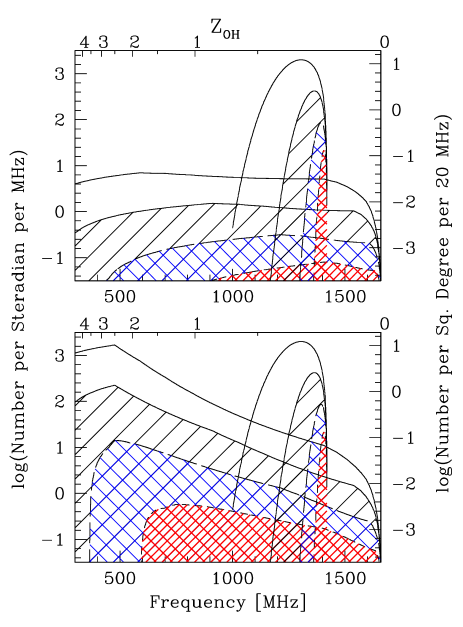
Figure 5: Detection rate as a function of frequency for two different redshift dependences of the merging rate. Top Panel   Constant merging rate. Bottom Panel   Merging rate proportional to $(1+z)^{4.5}$ for $z<2.5$ but constant for $z>2.5$. Detection rate is computed in a cosmological model with $\Omega_{o}=0.2$ for four sensitivity levels (0.2, 1, 5, and 20 mJy) for signals of velocity width 100 km s^-1. The lowest sensitivity survey (20 mJy) corresponds to the most heavily shaded area, and the highest sensitivity (0.2 mJy) is unshaded.

The importance of merging small galaxies to build the large galaxies that we observe at the present is a topic of considerable controversy, since the question addresses the foundations for theories of galaxy formation. In this section, it is demonstrated that surveys sensitive to OH masers at $z\approx 2$ may be able to measure the number density of interacting and merging systems at high redshift at a time when the merging rate is thought to peak. Observations using radio telescopes with sufficient sensitivity and sufficient spectral bandwidth can not only determine the statistics of the evolving density of OH masers with time, but they will also select systems of interest at high redshift, which can be further studied with a variety of techniques to determine physical conditions, dynamics and effects of local environment.

For the purposes of estimating the effect of an increased merging rate at early times, the model explored in Fig. 4 and the top panel of Fig. 5 can be modified by increasing the number density of OH megamasers in proportion to $(1+z)^{m}$, in keeping with the idea that, locally, OH megamasers are associated with luminous FIR galaxies, which in turn are found to occur in systems with merging and interacting morphologies (Clements et al 1996). For comparison, an extreme example, $m=4.5$ (Lavery et al 1996) is shown in Fig. 5. The significance of this detection rate is that an existing telescope, such as the Westerbork Synthesis Radio Telescope, which will reach a noise level below 1 mJy level in a 12 hour synthesis observation and can survey a field of one square degree per exposure at 600 MHz ($z_{oh}\approx 2$), would be likely to detect a few objects per field, when it is equipped with a spectrometer capable of 80 MHz (or more) bandwidth.

The luminous quasar population shows a still stronger evolution than is typically suggested for normal galaxies. Since the most luminous OH masers are associated with the most luminous galaxies in the nearby universe, it is reasonable to speculate about a possible relation between hosts for OH maser and quasars and the possibility that both may be driven by mergers and interactions. Figure 6 shows recent observational constraints on the comoving number density of bright QSOs ($M_{B}<-24.5$ $+5\log(h)$), as presented by Hewett et al (1993) for $z<2$ and Schmidt et al (1995) for $z>2.5$; these studies provide evidence that the comoving density peaked at $z\approx 2$ to 3. Representative curves for describing the increase in density $\phi_{-24.5}$ with redshift are drawn in the figure and indicate that $\phi_{-24.5}$ is roughly proportional to $(1+z)^{6}$ to redshift as high as $z\approx 2$. The QSO evolution is often described as an evolution in luminosity; Boyle et al (1988) quantify the QSO population as having a luminosity function $\phi_{qso}(L/L_{*})\propto\phi_{o}(L/L_{*})^{-3.7}$ with $L_{*}=L_{o}(1+z)^{3.2}$. Integrating to obtain the number of objects per comoving volume brighter than $L_{1}$ gives

$$N(>L_{1}) = \int^{\infty}_{L_{1}/L_{*}}\phi_{qso}\left(\frac{L}{L_{*}}\right)d\left(\frac{L}{L_{*}}\right)$$

$$= \frac{\phi_{o}}{2.7}\left(\frac{L_{1}}{L_{*}}\right)^{-2.7}$$

$$= \frac{\phi_{o}}{2.7}\left(\frac{L_{1}}{L_{o}}\right)^{-2.7}(1+z)^{5.9},$$

which has a proportionality that is consistent with the evolution for $z<2$ shown in Fig. 6 and in Schmidt et al (1995).

Figure 6: Comoving density of bright QSOs ($M_{B}<-24.5$ $+5\log(h)$) as a function of redshift. Points at $z<2.5$ are derived from Hewett et al (1993) (converted to $H_{o}=100$ km s^-1 Mps^-1); points at $z>2.5$ are adapted from Schmidt et al (1995). Three curves are drawn to indicate the evolutionary trend through the low redshift regime with the dependence $\propto(1+z)^{n}$ with $n=$ 2, 4 and 6.5. A horizontal dotted line is drawn to indicate a constant comoving density equal to the current density (see Fig. 1) of luminous OH sources ($L_{OH}>10^{4.1}h^{-2}L_{\odot}$ and $L_{60\mu}>10^{12.2}h^{-2}L_{\odot}$) that are bright enough to be detected at $z=3$ with 1 mJy sensitivity level.

The intention behind Fig. 6 is to show that at least one population of luminous object does evolve very steeply with redshift. An association between AGN activity and galaxy merging or interaction remains to be definitively established, although there is evidence that “warm,” ultraluminous infrared galaxies may be an evolutionary step in the evolution of optically selected QSOs (cf. Surace et al 1998). Interestingly, the $z\approx 0$ number density of ultraluminous FIR galaxies is comparable to the $z\approx 0$ density of luminous QSOs, as illustrated in the figure. Furthermore, Saunders et al (1990) deduced a density evolution ${\propto}(1+z)^{6.7}$ for their 60$\mu$m sample, although subsequent study by Ashby et al (1996) did not find the tail to high redshift expected if this were indeed the case. The evolution rate ${\propto}(1+z)^{4.5}$ explored in the lower panel of Fig. 5 is fairly mild in comparison to that of the QSOs.

4 Contamination of blind HI 21cm line surveys

Figures. 4 and 5 demonstrate that blind spectroscopic surveys are more likely to detect distant OH megamasers than HI from normal galaxies in the frequency bands below ${\sim}1200$MHz, assuming that both megamasers and normal galaxies have similar properties to those that are observed nearby. Above the rest frequency of the hydrogen line at $\nu_{HI}=$ 1420.4 MHz and in a small range of frequencies just below $\nu_{HI}$ there is a possibility for confusing OH emission at $z_{OH}\approx 1667/1420-1=0.17$ with weak HI signals from nearby dwarf galaxies and HI clouds. To explore this possibility in more detail, Fig. 7 shows a a plot similar to Fig. 5 with an expanded scale around 1420 MHz. The vertical axes have been adjusted to more convenient units to address this question. The possibility for confusion might arise in “blind surveys” for dwarf galaxies in the HI line, where signals at noise levels of a few $\sigma$ are selected as candidate dwarfs. At these sensitivity levels, only a narrow 1667 MHz might be detected, mimicing a narrow HI profile of a few 10’s of km s^-1 velocity width. Clearly more sensitive followup in the radio line, as well as far infrared and optical observations, would quickly show the distinction.

Figure 7: Detection rate of HI and OH signals near the rest frequency of neutral hydrogen. Two cases are illustrated for the faint end slope of the HI mass function, $\gamma=$ 1 and 1.3. Detection thresholds are set at 0.2, 1, 5 and 20 mJy.

Some questions remain about the slope of the luminosity function for galaxies at the faint end, and this uncertainty propagates into the faint galaxy tail of the HI-mass function as well. Recent HI surveys have produced values for $\gamma$ (as defined in Eq.(7)) in the range 1.2 to 1.7 (Zwaan et al 1997, Schneider 1997), although there is also observational evidence for a sharp decline in the number density of HI rich objects at faint HI luminosity (Hoffman et al 1992), at least in the Virgo cluster. Figure 7 implies that surveys with sensitivities of $\sim$1 mJy or better may be likely to detect OH masers (at $z_{OH}\approx 0.17$) in comparable numbers to the rate at which they detect weak HI signals in the velocity range $v_{HI}<500$ km s^-1.

This regime can be explored in more detail by estimating the form of the HI mass function that the OH masers would imitate. Figure 8 is an aid to visualize the problem. It shows a volume $dV_{OH}$ at $z_{OH}$ that is mapped into the volume $dV_{HI}$ at $z$ due to the overlap that occurs in observed frequency for the two populations. For simplicity in this estimate, approximations for the luminosity distance $d_{l}\approx z_{OH}c/H_{o}$ and for the comoving volume $dV_{OH}\approx z_{OH}^{2}dz_{OH}d\Omega$ will be assumed, instead of the more rigorous forms used earlier in this paper in the discussion of OH masers at cosmological distances. These produce errors of less than 10 percent in $d_{l}$ and less than 40 percent in comoving volume.

Figure 8: The volume $dV_{OH}\approx z_{OH}^{2}dz_{OH}d\Omega$ containing OH masers that is mapped into volume $dV_{HI}=z^{2}dz_{HI}d\Omega$ in HI surveys.

The incremental frequency band $d\nu$ observed at the frequency $\nu$ is related to increments in redshift for the OH and HI lines:

$$d\nu=-\frac{\nu^{2}}{\nu_{OH}}dz_{OH}=-\frac{\nu^{2}}{\nu_{HI}}dz_{HI}$$ (9)

implying that $dz_{OH}=(\nu_{OH}/\nu_{HI})dz_{HI}$. The flux $S$ measured in the line emission from the OH megamaser of luminosity $L_{OH}$ is falsely interpreted as HI emission from an object of $L_{HI}$:

$$S=\frac{L_{OH}}{4\pi(z_{OH}c/H_{o})^{2}}=\frac{L_{HI}}{4\pi(zc/H_{o})^{2}}$$ (10)

so that $L_{HI}=(z/z_{OH})^{2}L_{OH}$. Since the redshift range being explored for imitation HI signals is small, $z<0.01$, the OH masers are drawn from a thin shell, allowing $z_{OH}$ to be considered constant at $z_{OH}\approx 0.17$ in what follows.

The goal is to derive an approximation for the imitation HI mass function $\phi_{im}$ provided by distant OH masers. This can be accomplished by evaluating the number of signals that appear to come from the volume $dV_{HI}$ from emitters of strength $L_{HI}$ but which were actually produced in $dV_{OH}$ from emitters of $L_{OH}$. The relation between the luminosity functions then is $\Theta(L_{OH})dL_{OH}dV_{OH}=\phi_{im}(L_{HI})dL_{HI}dV_{HI}$. Solving for $\phi_{im}$, substituting from the above expressions as necessary and then including the approximate relation for the OH luminosity function from Eq.(2.2), which is valid here since all the OH signals detected will originate in emitters much brighter than $L_{OH}^{*}$:

$$\phi_{im} = \Theta(L_{OH})\left(\frac{dL_{OH}}{dL_{HI}}\right)\left(\frac{dV_{OH}}{dV_{HI}}\right)$$

$$= \Theta\left(\left(\frac{z_{OH}}{z}\right)^{2}L_{HI}\right)\left(\frac{z_{OH}}{z}\right)^{4}\frac{\nu_{OH}}{\nu_{HI}}$$

$$= \frac{C(\alpha+\beta)f_{m}}{2L_{OH}^{*}}\frac{\nu_{OH}}{\nu_{HI}}\left(\frac{L_{HI}}{2L_{OH}^{*}}\right)^{-\frac{\alpha+\beta+2}{2}}\left(\frac{z_{OH}}{z}\right)^{2-\alpha-\beta}$$

This result can then be recast as a dependence on $M_{HI}$:

$$\phi_{im}(M_{I})dM_{HI} = Cf_{m}\frac{\alpha+\beta}{2}\left(\frac{L_{OH}^{*}}{L_{HI}^{*}}\right)^{\frac{\alpha+\beta}{2}}$$ (12)

$${\times}\,\,\,\frac{\nu_{OH}}{\nu_{HI}}\left(\frac{M_{HI}}{M_{HI}^{*}}\right)^{-\frac{\alpha+\beta+2}{2}}$$

$${\times}\,\,\left(\frac{z}{z_{OH}}\right)^{\alpha+\beta-2}\frac{dM_{HI}}{M_{HI}^{*}}$$

After substitution for the constants in Eq.(12), $\phi_{im}$ has the functional dependence

$$\phi_{im}(M_{HI})dM_{HI} \propto \left(\frac{M_{HI}}{M_{HI}^{*}}\right)^{-2.15}\left(\frac{z}{z_{OH}}\right)^{0.3}\frac{dM_{HI}}{M_{HI}^{*}}$$ (13)

producing a form with that mimics a diverging low luminosity tail, since $(\alpha+\beta+2)/2=2.15$ is greater than 2. The dependence on $z$ does not affect the power law shape of the imitation mass function but does weakly affect the normalization that would be inferred.

The number of imitation HI masses per decade of $M_{HI}$ becomes

$$\hat{\phi}_{im}\approx 2.3{\times}10^{-5}\left(\frac{M_{HI}}{M_{HI}^{*}}\right)^{-1.15}\left(\frac{z}{z_{OH}}\right)^{0.3}{\rm Mpc}^{-3}$$ (14)

This estimate implies that a survey sensitive to 1 mJy signals, corresponding to $M_{HI}$ between $10^{5}$ and $10^{6}$M_⊙ at velocities of 300 to 500 km s^-1, would be unlikely to detect more than one imitator per cubic megaparsec. Therefore, with the current set of parameters describing the OH luminosity function, significant contamination of HI surveys at low redshift would only occur if the HI mass function turns out to be as flat as $\gamma\approx 1$ or drops off at low $M_{HI}$. Even substantial evolution in the merging rate from $z=0$ to 0.17 is unlikely to raise this density estimate by more than a factor of two, but some caution is in order until our understanding of the properties of OH masers improves. The likelihood for confusion might rise significantly if surveys were conducted at a 0.2 mJy sensitivity.

5 Conclusion

The density of OH megamaser galaxies in the sky may be high enough that radio spectroscopic surveys will be effective tools at identifying them. The time evolution of the megamaser sources could then be monitored by a series of surveys performed at a range of radio frequencies (i.e. different redshifts).

OH megamasers may form a source of confusion in surveys designed to detect neutral hydrogen in normal galaxies through their 21 cm emission. High resolution radio mapping, optical spectroscopy and far infrared detection would remove the ambiguity.

- [1]
- [2] Ashby M.L.N., Hacking P.B., Houck J.R., Soifer B.T., Weisstein E.W. 1996, ApJ 456, 428
- [3]
- [4] Baan W.A. 1989, ApJ 338, 804
- [5]
- [6] Baan W.A. 1997, in High Sensitivity Radio Astronomy, eds. Jackson, N., and Davis, R.J., Cambridge University Press, p. 73
- [7]
- [8] Baan W.A., Rhoads J., Fisher K., Altschuler D.R., Haschick A. 1992a, ApJ 396, L102
- [9]
- [10] Baan W.A., Haschick A., Henkel C. 1992b, AJ 103, 728
- [11]
- [12] Boyle B.J., Shanks T., Peterson B.A. 1988, MNRAS 235, 935
- [13]
- [14] Carlberg R.G., 1992, ApJ 399, L31
- [15]
- [16] Clements D.L., Sutherland W.J., McMahon R.G., Saunders W. 1996, MNRAS 279, 477
- [17]
- [18] Crane P.C., Napier P.J. 1989, in Synthesis Imaging in Radio Astronomy, eds. R.A. Perley, F.R. Schwab and A.H. Bridle, A.S.P. Conf. Series, 6, p. 139
- [19]
- [20] Henkel C., Baan W.A., Mauersberger R. 1991, A&AR 3, 47
- [21]
- [22] Hewett P.C., Foltz C.B., Chaffee F.H. 1993, ApJ 406, L43
- [23]
- [24] Hoffman G.L., Lu N.Y., Salpeter E.E. 1992, AJ 104, 2086
- [25]
- [26] Koranyi D.M., Strauss M.A. 1997, ApJ 477, 36
- [27]
- [28] Lavery R.J., Seitzer P., Suntzeff N.B., Walker A.R., Da Costa G.S. 1996, ApJ L1
- [29]
- [30] Martin J.-M., Bottinelli L., Dennefield M., et al. 1989, C.R. Acad.Sci, Paris, 308, 287
- [31]
- [32] Moshir M., Kopman G., Conrow T.A. 1992, IRAS Faint Source Survey, Explanatory supplement version 2, Pasadena: Infrared Processing and Analysis Center, California Institute of Technology.
- [33]
- [34] Neuschaefer L.W., Im M., Ratnatunga K.U., Griffiths R.E., Casertano S. 1997, ApJ 480, 59
- [35]
- [36] Norman C.A., Braun R. 1996, in Cold Gas at High Redshift, eds. Bremer M.N., van der Werf P.P., Röttgering H.J.A., Carilli C.L., (Kluwer Academic Publ.:Netherlands), pp 3-21
- [37]
- [38] Patton D.R., Pritchet C.J., Yee H.K.C., Ellingson E., Carlberg R.G. 1997, ApJ 475, 29
- [39]
- [40] Rowan-Robinson M. 1996, in Cold Gas at High Redshift, eds. Bremer M.N., van der Werf P.P., Röttgering H.J.A., Carilli C.L., (Kluwer Academic Publ.:Netherlands), pp 61-76
- [41]
- [42] Saunders W., Rowan-Robinson M., Lawrence A., et al. 1990, MNRAS 242, 318
- [43]
- [44] Schmidt M. Schneider D.P., Gunn J.E. 1995, AJ 110, 68
- [45]
- [46] Schneider S.E. 1997, PASA 14, 99.
- [47]
- [48] Staveley-Smith L., Norris R.P., Chapman J.M., et al. 1992, MNRAS 258, 725
- [49]
- [50] Surace J.A., Sanders D.B., Vacca W.D., Veilleux S., Mazzarella J.M. 1998, ApJ 492, 116
- [51]
- [52] Wieringa M.H., de Bruyn A.G., Katgert P. 1992, A&A 256, 331
- [53]
- [54] Zwaan M., Briggs F., Sprayberry D., Sorar E. 1997, ApJ 490, 173