25 Int. Cosmic Ray Conf., Durban 1997, Highlight Session
ADP-AT-97-9
VERY HIGH ENERGY GAMMA RAYS FROM MARKARIAN 501
R.J. Protheroe1, C.L. Bhat2,
P. Fleury3, E. Lorenz4, M. Teshima5, T.C. Weekes6
1Dept. of Physics and Math. Phys.,
University of Adelaide, Adelaide, SA 5005, Australia.
2Bhabha Atomic Research Centre, Mumbai - 400 085, India (on
behalf of the GRACE collab.)
3LPNHE - Ecole Polytechnique, 91128 Palaiseau, France (on
behalf of CAT Collab.)
4Max-Planck Inst.
für Physik, Munich, Germany (on behalf of HEGRA Collab.)
5Inst. for Cosmic Ray Research,
University of Tokyo, Japan (on behalf of TA Collab.)
6Harvard-Smithsonian CfA, Box 97, Amado, AZ 85645,
USA (on behalf of Whipple Collab.)
ABSTRACT
During remarkable flaring activity in 1997
Markarian 501 was the brightest source in the sky at TeV
energies, outshining the Crab Nebula by a factor of up to 10.
Periods of flaring activity each lasting a few days were observed
simultaneously by several gamma ray telescopes. Contemporaneous
multiwavelength observations in April 1997 show that a
substantial fraction of the total AGN power is at TeV energies
indicating that high energy processes dominate the energetics of
this object. Rapid variability, on time scales of less than a
day, and a flat spectrum extending up to at least 10 TeV
characterize this object. Results of 1997 observations by 6
telescopes are summarized and some of the implications of these
results are discussed.
1 INTRODUCTION
Markarian 501 is a classical Bl Lacertae object, a sub-classification of the Blazar class of AGN (core dominated, flat-spectrum radio, highly optically polarized and optically violently variable). It is the second closest known BL Lac () and like the closest, Markarian 421, it is a gamma-ray source. Both are classified as X-ray-selected BL Lacs and show virtually no emission lines.
It was first discovered as a TeV-emitting gamma-ray source by the
Whipple group in 1995 (Quinn et al. 1996). At that time, it had
not been detected by OSSE, COMPTEL or EGRET on the CGRO in any
observing period. At discovery the average TeV emission level
was 8% of the Crab Nebula and there was some evidence for daily
variability. In 1996 the emission level increased and there was
stronger evidence for variability (Quinn et al. 1997). The source
was confirmed as a TeV source by the HEGRA group (Bradbury et
al. 1997).
2 OBSERVATIONS DURING 1997
In January, 1997 the Whipple group noted that it was brighter than usual in low elevation observations. This was confirmed in February, 1997 and the HEGRA, CAT and TA groups were alerted. After confirmation by HEGRA and CAT the three groups sent out a joint notification as an IAU Circular (Breslin et al. 1997). The nightly averages, plotted as fraction of the Crab rate, as seen by the Whipple Collaboration in 1995, 1996 and 1997, are plotted in Figure 1. The average level from February through June, 1997 was four times that of the Crab, an increase by a factor of 50 on the discovery level in 1995.

If the 1997 Whipple observations are broken down by night into individual 28 minute runs, there is evidence on seven nights for significant variations using a Chi Square test. On two of these nights the significance level of the variations is a few times after allowing for the number of trials (Quinn, 1997). The doubling time is approximately 2 hours.
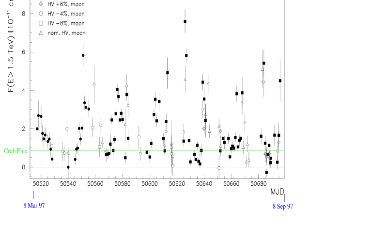
Figure 2a shows the light curve obtained with HEGRA CT-System. Normally, optical Cherenkov observations are not carried out if the Moon is visible as this increases dramatically the night sky brightness. However, because of the strength of the gamma-ray signal from Markarian 501 the HEGRA group continued observing during moonlight using CT1 but with a higher energy threshold. The complete light curve of Markarian 501 between 8 March 1997 and 9 September 1997 as observed by HEGRA CT1 is shown in Figure 2b. The different symbols indicate under which conditions the observations were made. In the calculation of the flux, differences in the calibration were taken into account.
TACTIC is a compact array of 4 Cherenkov telescopes located at Mt. Abu, India. During its first observing campaign in April-May, TACTIC observed Markarian-501 with a statistical significance of 14.2. The corresponding source light curve is displayed in Figure 3a.


CAT is an optical Cherenkov telescope located in the French Pyrenees. The large number of small diameter pixels in the camera allows a relatively small mirror (5 m diameter), compared to the Whipple telescope, to achieve a low energy threshold. CAT also saw Markarian 501 during its inaugural observing period and the light curve is obtained is shown in Figure 3b.
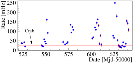
Observations of TeV gamma ray from Markarian 501 were made using the Telescope Array (TA) prototype located at Dugway, Utah, from the end of March to end of July. They observed on a total number of 47 nights. The gamma ray event rate is plotted as a function of MJD in Figure 3c. For reference, the gamma ray rate from Crab measured by our detectors is shown by the horizontal line. The event rate is highly variable day by day, and the maximum event rate is about 5 Crab and the minimum rate is Crab.
Details of these telescopes and their observations of Markarian 501 are given in Table 1.
Table 1: Telescopes used for Markarian 501 observations.
Telescope:
Whipple
HEGRA
CAT
TA
TACTIC
CT-System
CT1
Site:
Mt Hopkins
La Palma
La Palma
Thémis
Dugway
Mt Abu
Longitude(∘E):
-110.53
-17.8
-17.8
-2.0
-113.02
+72.7
Latitude (∘N):
31.41
28.8
28.8
42.5
40.33
24.6
Elevation (m):
2300
2240
2240
1650
1600
1300
# telescopes:
1
4
1
1
3
4
Mirror area (m2):
74.0
5.0
17.5
# pixels:
151
127
548 (+52)
256
81
Pixel diameter (∘):
0.25
0.24
0.24
0.12
0.25
0.31
Threshold (GeV):
300
500
1500
300
600
700
Total observation:
67.7 h
150 h
250 h
88 h
105.4 h
50.1 h
February:
3.4 h
–
–
0.8 h
–
–
March:
10.7 h
yes
yes
16.3 h
yes
–
April:
21.4 h
yes
yes
39.0 h
yes
22.54 h
May:
19.8 h
yes
yes
7.8 h
yes
27.51 h
June:
12.4 h
yes
yes
11.4 h
yes
–
July:
–
yes
yes
5.3 h
yes
–
August:
–
–
yes
5.4 h
–
–
September:
–
–
yes
2.0 h
–
–
In addition, Markarian 501 has been detected by the University of Durham telescope at Narrabri, Australia, by observing at extremely large zenith angles (). The source was also observed by the high elevation Tibet AS- air shower array which has a threshold at 10 TeV, making this the first detection of an AGN by an air shower array.
3 LIGHT CURVES
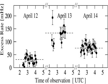
All of the reported light curves (Figures 1, 2 and 3) show excellent morphological similarity, with flaring episodes of several days when the flux is higher than average, but also with dramatic day to day variability. For example, the flaring episodes in March April, May and June were observed by all telescopes operating at that time. In addition to this daily flaring, variability over periods of hours is also seen. For example, using the CT-System the HEGRA group investigated the light curve on sub-hour time scales, and this is shown for the April flare in Figure 4a.

The long term behaviour (1995–1997) obtained by Whipple has been shown in Figure 1 illustrating an increase from year to year. Figure 4b shows the HEGRA CT1 flux averaged over periods of 30 days (due to the large daily fluctuations of the flux, the average flux has large statistical errors). Although there is a faint decay trend visible in the last four months of data, the light curve averaged over 30 days is consistent with a constant emission level during 1997.
The episodes of flaring lasting several days have occurred almost
every month, and this may indicate either a periodic or
quasiperiodic process. For example, looking at the HEGRA CT1
light curve (Fig. 2b) we see minima every days.
Looking at the TA light curve (Figure 3c) we can see high states
and low states clearly the data. This feature (the time scale
and the intensity change) in April and in July appear to be
similar, showing “U” shapes, and the interval between the two
high states are 14 days and 12 days. The May and June data each
show only one high state with a “” shape suggestive of
a possible day periodicity. Using the Rayleigh
test, the TA group obtain a 12.7 day period with an estimated
chance probability of less than . However, this period
requires a flare on April 13 and flaring on that day was seen by
Whipple, but both CAT and Whipple see a stronger flare on April
16. One should also worry about possible aliasing due to gaps in
the time series (day time and full moon periods). Thus while
very interesting, the possible periodicity should be treated as
very preliminary.
4 ENERGY SPECTRUM
Using the same analysis as was used for the Crab spectrum (Carter-Lewis et al. 1997) and the Markarian 421 spectrum (McEnery et al. 1997), a preliminary energy spectrum for the Whipple observations was derived based on 255 minutes of data (nine ON/OFF pairs) taken in April, 1997. The resulting spectrum can be represented by:
| (1) |
The errors shown are purely statistical. The systematic errors are at least as large since these observations were made with an expanded 151-pixel camera which has not yet been fully characterized.
A series of observations at low elevations was made at Whipple to extend the energy coverage to higher energies. These resulted in a detection in which 90% of the gamma rays were above 8 TeV (median energy 12 TeV) and a detection in which 90% were above 10 TeV with a median energy of 15 TeV. It is not yet possible to derive an energy spectrum and absolute flux with this technique.
Figure 5a shows the preliminary energy spectrum obtained by HEGRA CT1 in 1997 and is compared to that obtained in 1996. While in 1996 a differential spectral index of was measured (open circles), the 1997 spectrum seems to be steeper. The excess rate is essentially unchanged around 10 TeV. Further analysis of the spectrum is underway.
The CAT group have obtained energy spectra during the April 15/16 flare, between flares, and for all the data (Fig. 5b). Fits between 200 GeV and 2 TeV for the 3 cases give differential fluxes at 1 TeV ( m-2 s-1 TeV-1) of , , and respectively. The corresponding spectral indices were , and .


The differential energy spectrum obtained by the TA is shown in Figure 5c and can be expressed m-2 s-1 TeV-1. The spectrum becomes steeper above 5 TeV which may suggest a cut off of the energy spectrum, although it is possible that statistical fluctuations may cause this effect. More statistics are needed to obtain conclusive results.
The estimated time-averaged flux obtained from TACTIC
observations (April 9 - May 30, 1997) above a gamma-ray threshold
energy of TeV is nearly 2 Crab units, in
excellent agreement with the source spectrum inferred for the
corresponding period from independent observations by the HEGRA,
CAT and the Whipple groups.
5 MULTI-WAVELENGTH OBSERVATIONS
As a result of the high activity on Markarian 501 in March, 1997 a Target of Opportunity was declared for CGRO to observe the source with all instruments for the period April 9-16. As observed by several telescopes, Markarian 501 was very active during this period in TeV gamma-rays with peaks on April 13 and 16; the flux level on April 16 was photons per minute. The TeV light curve observed by Whipple, CAT and HEGRA is shown in Figure 6a. Note that HEGRA missed the flare on April 16 due to cloudy sky.

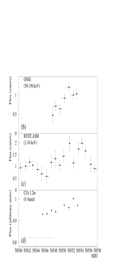
An analysis of the EGRET observations shows no statistically significant evidence for emission, and an upper limit of photons cm-2 s-1 was derived. There was no report from COMPTEL, but OSSE, operating in the 0.05-10 MeV range, saw a strong signal (Fig. 6b). The daily flux varied by a factor of 2 (compared with the factor of 4 at TeV energies). In the 50-150 KeV range OSSE saw the strongest signal seen from any blazar. The spectral index is steep compared to other blazars observed by OSSE (Figure 7).


The source was also observed by the RXTE (Catanese 1997) and Beppo
SAX (Pian et al. 1997) X-ray telescopes and the results will be
presented elsewhere. Results from the ASM detector on RXTE are
shown in Fig. 6c. There is a clear correlation between the
variations seen at TeV energies and those seen in X-rays; however
the amplitude of the variations is smaller at the longer
wavelengths. There is also weak evidence for correlation with
variations in the optical U-band (Fig. 6d).
6 INTERPRETATION AND CONCLUSION
The composite spectrum is shown in Figure 7. The double peak (at UV-X-ray and gamma-ray energies) is characteristic of gamma-ray emitting blazars; however the longer wavelength peak is shifted to higher energies compared with Markarian 421 and other blazars. Compared to the 1 keV cut-off in Markarian 421 the Markarian 501 cut-off is keV, implying in a Compton-synchrotron model that the electrons have very high energies. In this case, the lack of detection of 100 MeV gamma rays by EGRET results from this energy falling between the synchrotron and inverse Compton peaks.
The very rapid time-variability observed places strong constraints on models of gamma-ray emission. The fact that only blazars appear to show strong gamma ray emission, and that this class of AGN has relativistic jets closely aligned with the line of sight, strongly suggests the gamma rays originate in an emission region in the jet. Because of the lack of emission lines it is likely that much of the lower energy radiation is also non-thermal. In the homogeneous synchrotron-self Compton model the low energy photons are produced in the same region as the high energy emission. We shall consider the emission region to be a “blob” or radius moving relativistically along the jet axis with velocity and Lorentz factor , and containing a population of relativistic electrons, magnetic field and radiation.
If an AGN at redshift is observed at angle to the jet axis and the blob emits two pulses of light separated by blob-frame time (blob frame quantities are primed), the observed arrival times of the two pulses will be separated by where
| (2) |
is the “Doppler factor”. The energies of emitted photons are also boosted in energy as a result of the bulk motion of the blob such that .
If is the fastest observed variability time, and we assume the emissivity varies with time uniformly over the blob, then the radius of the blob can not be much larger than . Then the differential photon number density at energy in the blob frame per unit photon energy is approximately
| (3) |
where is the observed differential photon flux at energy and is the luminosity distance. If the Doppler factor is too small then the photon density in the blob frame may be so large that gamma-rays may not escape due to photon-photon collisions. The optical depth for this process depends on energy and is given by
| (4) |
where , and is the cross section for photon-photon pair production at centre of momentum frame energy squared . During April the 2–10 keV and 15–150 keV fluxes were at roughly the same level with the 2–10 keV flux being about 5 times higher than the archival data. Assuming the lower energy fluxes increased by about the same amount, one obtains the spectral energy distribution given by the dotted curve which has been added to Figure 7. One can then calculate the minimum Doppler factor as a function of gamma-ray energy, such that , for any given variability time scale. This has been done for day, 1 hour, and 15 minutes (Bednarek and Protheroe 1998) and is shown in Figure 8. We note that for a 15 minute variability time scale and a gamma ray spectrum extending to 20 TeV that a Doppler factor of at least about 30 is required.

Gamma ray emission from active galactic nuclei (AGN) is often interpreted in terms of the homogeneous synchrotron self-Compton model (SSC) in which the low energy emission (from radio to X-rays) is synchrotron radiation produced by electrons which also up-scatter these low energy photons into high energy -rays by inverse Compton scattering (IC) (Macomb et al. 1995, Inoue & Takahara 1996, Bloom & Marscher 1996, Mastichiadis & Kirk 1997). In this model all the radiation comes from this same region in the jet. Such a picture can naturally explain synchronized variability at different photon energies and has been tested in the context of Markarian 421 (Bednarek and Protheroe 1997a). More complicated (inhomogeneous) SSC models are also proposed which postulate that the radiation at different energies is produced in different regions of the jet (e.g. Ghisellini et al. 1985, Maraschi et al. 1992).
In the SSC model the spectral energy distribution has two broad peaks. The low energy component is due to synchrotron emission, and the high energy component being due to inverse Compton scattering of the low energy component by the same electrons that produce the synchrotron radiation. We identify the low energy component with the photon spectrum extending up to MeV observed by OSSE, and the high energy component with the TeV gamma rays. The inverse Compton scattering producing the highest energy gamma rays at TeV will be in the Klein-Nishina regime where the scattered photon energy is comparable to the maximum electron energy. Thus
| (5) |
where is the maximum electron energy in the jet frame. Thus we obtain for and TeV.
The maximum energy of the low energy component will be determined by the magnetic field in the blob and by and is given approximately by
| (6) |
where , and G. Thus we can obtain the magnetic field in the blob,
| (7) |
which gives G for , and MeV.
To obtain the observed variability time (in particular the observed fall time of the gamma ray signal) the highest energy electrons must be able to convert their energy into radiation in a time less than that observed. Thus we require at least that
| (8) |
We now have an estimate of the differential photon number density and the magnetic field in the blob, and are able to calculate the cooling times of electrons by inverse Compton scattering and synchrotron radiation. The cooling time in the blob frame for each process is given by
| (9) |
where is either erg cm-3 which is the magnetic energy density (synchrotron losses) or
| (10) |
which is the energy density of photons which will scatter in the Thomson regime, where . Thus we obtain fall times in the observer’s frame of s and 50 s for inverse Compton and synchrotron respectively, which are consistent with the observed variability time scale of several minutes.
We should also check whether electrons can be accelerated up to the maximum energy given the magnetic field present in the blob. This depends on their acceleration rate
| (11) |
where is the acceleration efficiency which depends on the mechanism, and on the synchrotron plus IC energy loss rate
| (12) |
where . Equating to we obtain
| (13) |
For we require . Such an acceleration efficiency is quite reasonable for shock acceleration.
The acceleration time should be consistent with the rise time of the the observed gamma ray signals, i.e. . The acceleration time is given by
| (14) |
and for , G, and we obtain s which is again consistent with the observed rise time.
From the discussion above one would conclude that the SSC model can give a satisfactory explanation for the present observations of Markarian 501. However, the model parameters are rather finely balanced. The comparable cooling times for inverse Compton and synchrotron radiation lead to similar power being emitted at TeV energies and sub-MeV energies as was observed during April 1997 (see Fig. 7). If, however, more rapid variability were observed or much higher energy gamma rays were detected on the same variability time scale, then the minimum Doppler factor required for gamma ray escape would increase (see Fig. 8) such that the SSC model could be in trouble. The reason for this is that the balance between for synchrotron and IC (which are proportional to and ) is disturbed. For example, from Eq. 5, and from Eq. 6 giving , while . Thus the ratio of the power going into the high energy component to that going into the low energy component is proportional to . Increasing by 50% causes this ratio go down by a factor of 10. One should also not overlook other possible scenarios such as hadronic models (Mannheim 1995, Protheroe 1996) which can be tested by searching for correlated high energy neutrino emission.
If the 13 day or 29 day periodicity suggested by the analysis of the TA and HEGRA light curves is confirmed it will provide important constraints on the emission region/mechanism. One possibility under consideration (Protheroe 1998) is that this may arise if the jet has internal helical structure, or is helical as has been suggested by Conway and Wrobel (1995) based on the observed mis-alignment of the pc scale and kpc scale jets in Markarian 501. However, for this to work, i.e. to give the periodicity and for the jet to have the observed jet mis-alignment, one would require a helix wavelength of about 50 kpc, a viewing angle of , and a jet Lorentz factor of .
Finally, we mention some alternative scenarios which might
possibly explain the rapid variability observed in both Markarian 421
and Markarian 501. Bednarek and Protheroe (1997b,1997c) have suggested
that this could arise as a result of the interaction of stars
with the jet, or as a result of time dependent gamma ray
absorption by collisions of the gamma rays with photons from from
a hot-spot on an accretion disk.
7 REFERENCES
Bednarek, W., and Protheroe, R.J., (1997a) MNRAS, in press
Bednarek, W., and Protheroe, R.J., (1997b) MNRAS, 287, L9
Bednarek, W., and Protheroe, R.J., (1997c) MNRAS, 290, 139
Bednarek, W., and Protheroe, R.J., (1998) MNRAS, in preparation
Bloom, S.D., Marscher, A.P., (1996) ApJ 461, 657
Bradbury, S.M. et al. (1997) A&A, 320, L5.
Breslin, A.C. et al. (1997) IAU Circ. 6596.
Carter-Lewis, D.A. et al., (1997) 25th ICRC (Durban), 3, 161.
Catanese, M. (1997) in preparation.
Catanese, M., et al. (1997) ApJL (in press).
Conway, J.E., and Wrobel, J.M., (1995) Ap.J., 439, 112
Ghisellini, G., Maraschi, L., Treves, A., (1985) A&A, 146, 204
Inoue, S., Takahara, F., (1996) ApJ 463, 555
Macomb, D.J. et al., (1995) ApJ, 449, L99 (Erratum 1996, ApJ 459, L111)
Mannheim, K, (1995) Astroparticle Phys., 3, 295
Maraschi, L., Ghisellini, G., Celloti, A., (1992) ApJ 397, L5
McEnery, J. et al. (1997) 25th ICRC (Durban) 3, 257.
Mastichiadis, A., Kirk, J.G., (1997) A&A, in press
Pian, E., et al. (1997) ApJL, submitted.
Protheroe, R.J., (1996) in Proc. IAU Colloq. 163, Accretion
Phenomena and Related Outflows,
ed. D. Wickramasinghe et al., in press
Protheroe, R.J. (1998) in preparation.
Quinn, J. et al. (1996) ApJ, 456, L83.
Quinn, J. et al. (1997) 25th ICRC, 3, 249.
Quinn, J. (1997) National University of Ireland, Ph.D. Dissertation
(unpublished).