Keck Spectroscopy of Globular Clusters around NGC 1399¹

Abstract

We report moderate resolution, high signal–to–noise spectroscopy of globular clusters around NGC 1399, the central cD galaxy in the Fornax cluster. We address issues as diverse as element abundances of globular clusters versus stellar populations in ellipticals, blue horizontal branches in metal–rich globular clusters, broad–band colors as metallicity tracers, possible overestimation of the age–metallicity degeneracy in globular clusters, and dark matter in the halo of NGC 1399.

We obtained spectra for 21 globular cluster candidates with multi-slit spectroscopy using the LRIS on the KECK 1 telescope. Our sample turned out to include 18 globular clusters, 1 star, and 2 low redshift late-type galaxies ($z\simeq 0.3$).

The mean velocity of our globular cluster sample is $1293\pm 71$ km$\cdot$s^-1 and its velocity dispersion $302\pm 51$ km$\cdot$s^-1. Both are slightly lower than, but in agreement with, previously derived values. We derive a mass of 1 to $5\times 10^{12}M_{\odot}$ within 28 kpc for the galaxy, and a $M/L_{\rm B}$ ratio of $36\pm 20$ or $76\pm 40$ $M_{\odot}/L_{\odot\rm B}$, depending on the mass estimator. Both estimates indicate that dark matter dominates the potential at 6 r_eff.

The derived element abundances for the globular clusters span the entire range observed in the Milky Way and M31, with a mean metallicity of our sample around $[$Fe/H$]\simeq-0.8$ dex. This implies that the two major sub–populations reported from photometry could have formed by the same processes as the ones that formed halo and disk/bulge globular clusters in the Local Group spirals. Two globular clusters (that we associate with a group of very red globular clusters, representing about 5% of the total system) clearly stand out and exhibit metal abundances as high as observed for stellar populations in giant ellipticals. In addition, they display surprisingly high H$\beta$ and H$\gamma$ indices that are not explained by any age/metallicity combination of existing models. The high Mg and H$\beta$ values in these clusters could, however, be explained by the presence of blue horizontal branches.

Finally, we find that V$-$I and metallicity are well correlated in the globular cluster system, but that the slope of the relation is twice as flat at high metallicities as an extrapolation from the relation for Milky Way globular clusters. This implies that the mean metallicities of globular cluster systems in ellipticals are lower, and cover a smaller range, than previously derived from broad–band V$-$I colors.

to appear in the Astronomical Journal (January 1998 issue) Kissler-Patig et al. Keck Spectroscopy of Globular Clusters around NGC 1399

and

1 Introduction

Globular cluster systems were extensively studied using photometry in the last two decades producing many interesting findings (e.g. Ashman & Zepf 1997 for a review). However, many new questions were raised that could not be answered using broad–band colors alone because population synthesis models predict (sometimes strong) age–metallicity degeneracies (e.g. Worthey 1994). Several attempts were made to obtain spectra of globular clusters in systems outside the Local Group (Mould et al. 1987, Mould et al. 1990, Huchra & Brodie 1987, Brodie & Huchra 1991, Grillmair et al. 1994, Perelmuter, Brodie & Huchra 1995, Hui et al. 1995, Bridges et al. 1997, Minniti et al. 1998). However, all of these studies had to focus on the very brightest globular clusters in the host galaxies and only low signal–to–noise spectra were obtained. Kinematic information could be obtained for the globular clusters but, for the vast majority, line indices were either affected by high photon noise, or not measurable at all.

Using the new generation of 10m–class telescopes, the expectation was that reliable line indices would be measurable for many globular clusters in galaxies at typical distances of the Virgo or Fornax galaxy clusters. Among the open questions were: Do globular clusters in other galaxies show the same abundances and abundance ratios as in the Local Group, i.e. can they have formed by similar processes? Are globular clusters in ellipticals more metal rich than in spirals as thought from their broad–band colors (e.g first pointed out by Cohen 1988), and what is the upper metallicity limit? Can the abundances help to identify a population of globular clusters in ellipticals that formed during a merger event? How do the abundances of globular clusters relate to those of the stars of the host galaxies? Preliminary answers to some of these questions were discussed by Brodie & Huchra (1991), but conclusive statements require better data than was available to them.

Here we report the first spectroscopically derived abundances for globular clusters in NGC 1399, the central giant elliptical galaxy in Fornax. NGC 1399, like other cD galaxies, has an over–abundant globular cluster system with $\simeq 5800$ globular clusters (Kissler-Patig et al. 1997, Forbes et al. 1997). Photometric studies suggest the presence of multiple globular cluster sub–populations (e.g. Ostrov et al. 1993, Kissler-Patig et al. 1997, Forbes et al. 1997), the origins of which are uncertain. In the next section we describe the observations. In section 3 we derive the kinematics of our globular cluster sample and use this information to give an estimate of the galaxy mass and mass–to–light ratio at several effective radii. The abundances and metallicities of our globular clusters are derived in Sect. 4. In section 5 we discuss our broad–band colors together with the line indices. We draw conclusions from our sample in Sect. 6.

2 Observations and Reduction

We selected 21 globular cluster candidates from the original list used by Grillmair et al. (1994) and kindly provided by W. Couch. These cluster candidates were identified on deep photographic plates in the Anglo-Australian Telescope archive and were selected on the basis of their B${}_{j}-$R colors.

The observations were carried out with the Low Resolution Imaging Spectrograph (LRIS, Oke et al. 1995) in multi-slit mode at the Keck 1 telescope on the nights of 1995, December 22nd and 23rd. Exposures totaling 160 min were taken over the two nights for one mask with 21 slitlets + 3 centering objects. Comparison lamps and flat fields were taken after the 30 min + 20 min exposures on the night of the 22nd, and before and after the 20 min + $3\times 30$ min exposures in the night of the 23rd.

The CCD used was a Tektronix 2048$\times$2048 with 24 $\mu$m pixels. The observations were made with a 600g/mm grating (blazed at 5000 Å, with a dispersion 1.24Å/pixel) and 1 arcsec slitlets, resulting in an effective resolution of 5.6Å  and a usable wavelength range of 4000Å to 6100Å common to all spectra.

The reduction was done in a standard fashion under IRAF, with the help of Kelson’s et al. (1997) EXPECTOR program. Every exposure was bias–corrected using an average of bias exposures taken at the beginning and end of the night, adjusted to the overscan region of each image. The exposures were then divided by internal lamp flatfields, that were averaged and normalized to a value of unity for each slitlet individually, in order to correct for wavelength response. The flatfielded 2–D images were then corrected for the instrument x and y distortions by constructing a distortion map from the flatfield and comparison lamp exposures that was then applied to the science exposures. The wavelength calibration and sky subtraction was carried out by the EXPECTOR program. The wavelength solution was obtained from 25–30 Hg, Ar, Ne, and Kr lines in the comparison lamp spectra taken before and after the series of science exposures and shifted versus the night sky lines on the sciences exposures. The wavelength solution fitted by a third order Legendre polynomial, had a typical 1$\sigma$ rms below 0.2 Å ($\simeq 10$ km$\cdot$ s^-1) in the region redward of 4800 Å where it could be well–anchored to night sky lines. Below 4500 Å the wavelength solution was less well–defined and could deviate at the blue end by up to 1 Å. The sky subtraction blueward of 5500 Å, where only a few weak sky lines are present, worked very well and between 5500Å and 6100Å only the expected photon noise from the brightest Oxygen and Sodium night sky lines remained after the subtraction. The individual wavelength–calibrated spectra were then extracted under IRAF and averaged to produce high signal to noise spectra.

The flux calibration was done using long slit data of the flux standard Feige 25, observed before the target exposures on the same nights as the targets. The response curve seems to vary slightly with the position of the spectra on the chip, so that velocities and line indices were measured both on the flux calibrated and flux uncalibrated (hereafter fluxed and unfluxed) spectra. For all objects the results agreed within small fractions of the errors. Values quoted below for velocities and line indices are the average of the two methods.

3 Radial Velocities of the globular clusters

3.1 Radial velocity measurements

The final spectra were cross-correlated with two velocity template spectra obtained during the same run (M31 globular clusters 225-280, $v_{helio}=-164$ km$\cdot$s^-1 and 158-213, $v_{helio}=-180$ km$\cdot$s^-1) using the method of Tonry & Davis (1979) implemented in the FXCOR package within IRAF. Only the spectral region between 4800 Å and 6000 Å was used as this is where the wavelength solution is best defined. In most cases the cross–correlation peaks were very well defined and the formal errors returned by the cross–correlation were on the order of 25 km s^-1. Combined with the errors in the wavelength calibration, we estimate the random error to be on the order of 30 km s^-1. We checked for any systematic errors in the reduction of the individual objects by using individual exposures instead of the combined spectra, and using different comparison lamp spectra for the wavelength calibration. The dispersion of these individual measurements was added in quadrature to the formal error. This total error is given in Table 1, together with the heliocentric velocity, V magnitude and V-I color taken from the NW field of Kissler-Patig et al. (1997), the photographic B_j magnitude and B${}_{j}-$R color from the original list used by Grillmair et al. (1994) and, for the five objects in common, the velocity quoted by Grillmair et al. (1994). Note that the objects #4, #8, and #16 turned out to be a star and two low–redshift early–type galaxies, and will not be discussed in the following. Figure 1 shows our velocities versus those of Grillmair et al. (1994) for the five objects in common. The velocities are in good agreement, within the errors, and no systematic shift can be identified in this sample. We plotted the location of our globular clusters with respect to the galaxy in Fig. 2, where the rings indicate 1 and 5 galactic effective radii (taken from Goudfrooij et al. 1994) and the sizes of the symbols reflect the globular cluster velocities with respect to the mean sample velocity (open being approaching, solid being receding). Our globular clusters are located between 2 and 7 effective radii of the galaxy and extend from the North to the West of the galaxy.

3.2 Globular cluster velocities

A histogram of the globular cluster velocities is shown in Fig. 3. The mean velocity of our sample is 1293 $\pm 71$ km$\cdot$s^-1, that is offset by 150 km$\cdot$s^-1 from the systemic velocity of NGC 1399 (1447 km$\cdot$s^-1, de Vaucouleurs et al. 1991). The mean velocities of previous samples are 1517 $\pm 91$ km$\cdot$s^-1 (Grillmair et al. 1994) and 1353 $\pm 79$ km$\cdot$s^-1 (or 1309 $\pm 71$ km$\cdot$s^-1 without an outlier, Minniti et al. 1998). The latter sample is mainly situated on the opposite side of the galaxy from ours (South East of the galaxy), making it unlikely that rotation is the cause of our low mean velocity. This is further supported by the results of Grillmair et al. (1994), who found no evidence for rotation in their more uniformly distributed sample.

The velocity dispersion derived from our sample is 302 $\pm 51$ km$\cdot$s^-1. It is slightly lower than, but consistent within the errors with, the ones derived by Grillmair et al. (1994): $388\pm 54$ km$\cdot$s^-1, and Minniti et al. (1998): $338\pm 56$ km$\cdot$s^-1 (or $293\pm 50$ km$\cdot$s^-1 without an outlier). As noted in the previous studies, the velocity dispersion is higher than measured for the stellar component within 1.5 arcmin, suggesting that either the mass–to–light ratio and/or radial anisotropy changes dramatically between 1.5 and 5 arcmin.

Figure 4 shows magnitude and color versus velocity. Figure 5 shows velocity versus radius. Given the small size of our sample only very clear correlations would be discernible. Apparently velocity does not strongly correlate with radius, color or magnitude of the globular clusters. Such correlations will be explored more fully in a forthcoming paper which will including all three (Grillmair et al. 1994, Minniti et al. 1998, and this work) globular clusters samples (Kissler-Patig et al. 1998).

3.3 Mass estimate and the Mass–to–Light ratio

3.3.1 Mass estimate

The velocity distribution of the globular clusters can be used to give an estimate of the mass of the parent galaxy. Given the small number of velocities and the poor spatial coverage, we follow a simple method also applied by Huchra and Brodie (1987). We estimate the mass from the virial theorem on the one hand, and from the projected mass method on the other hand (Bahcall & Tremaine 1981, Heisler, Tremaine & Bahcall 1985). The virial theorem mass for a system of $N$ globular clusters with measured velocities is

$$M_{\rm VT}=\frac{3\pi N}{2G}\frac{\Sigma_{i}^{N}V^{2}_{i}}{\Sigma_{i<j}1/r_{ij}}$$ (1)

where $r_{ij}$ is the separation between the $i$th and $j$th cluster, and $V_{i}$ is the velocity difference between the $i$th cluster and the mean system velocity. The projected mass is

$$M_{P}=\frac{f_{p}}{G(N-\alpha)}(\Sigma_{i}^{N}V_{i}^{2}r_{i})$$ (2)

where $r_{i}$ is the separation of the $i$th globular cluster from the centroid. The quantity $\alpha$ was chosen to be 1.5 following Heisler et al. (1985), as a slight correction to $f_{p}$, used in a discrete model but determined analytically from a continuous model. The quantity $f_{p}$ depends on the distribution of the orbital eccentricities for the globular clusters, it ranges from to $64/\pi$ for radial orbits, over $32/\pi$ for isotropic orbits, to $64/3\pi$ for circular orbits, in an extended mass. We adopt a projection factor of $32/\pi$, which assumes purely isotropic cluster orbits in an extended mass, for comparison with the simulations of Hernquist & Bolte (1993).

The results from both methods are: $M_{\rm VT}=2.0(\pm 0.9)\cdot 10^{12}M_{\odot}$ and $M_{P}=4.3(\pm 1.0)\cdot 10^{12}M_{\odot}$ within a radius of 5 arcmin or 28 kpc, adopting a distance to NGC 1399 of 19.3 Mpc (Madore et al. 1997).

The errors were calculated by a standard jackknife procedure (e.g. Efron & Tibshirani 1993). Further, we have to consider the incomplete spatial coverage of our sample. We derived the effective radius of the globular cluster system by fitting a de Vaucouleurs profile to the globular cluster surface density data of Kissler-Patig et al. (1997). We obtained an effective radius r${}_{\rm eff(GCS)}=120"\pm 20"$. The mean radius of the spectroscopic sample is $\simeq 1.6$ r_eff(GCS). Richestone & Tremaine (1984) showed that a single velocity dispersion observed at 1.6 r_eff (approximating our observations) can vary by a factor of $\simeq 1.8$. Thus, mass–to–light ratios derived from observations like ours can vary by a factor $\simeq 3.2$. An additional error might be present in the projected mass method: Hernquist and Bolte (1993) simulated a globular cluster distribution around a galaxy and noted that a sample like ours (roughly 20 objects extending out to 30 kpc, assuming $f_{p}=32/\pi$), systematically overestimates the total galaxy mass by up to 50%. In addition, the value we adopted for the projection factor was assumed without knowledge of the real globular cluster orbits.

3.3.2 The Mass–to–Light ratio

The total luminosity within 5 arcmin is obtained from the light profile of Bicknell et al. (1989), correcting for our assumed distance of 19.3 Mpc. We obtain a total integrated luminosity within 5 arcmin of $5.5(\pm 0.5)\cdot 10^{10}L_{\odot\rm B}$ and estimate a mass to light ratio within 28 kpc of $M/L_{B}\simeq 36\pm 20M_{\odot}/L_{\odot}$ using $M_{\rm VT}$ or $M/L_{B}\simeq 76\pm 40M_{\odot}/L_{\odot}$ (likely to be an overestimate, see above) using $M_{P}$.

Grillmair et al. (1994) derived $M/L_{B}=79\pm 20M_{\odot}/L_{\odot}$, but assumed a distance to NGC 1399 of 13.2 Mpc, i.e. their value would fall around $M/L_{B}\simeq 35M_{\odot}/L_{\odot}$ for our assumed distance. Minniti et al. (1998) derived $M/L_{\rm B}$ values between 50 and 130, also assuming a slightly shorter distance. All samples cover comparable galactocentric distances. In summary the values agree when corrected for the different assumed distances. The main result is that this mass–to–light ratio is about a factor 10 above that expected for an old stellar population, leading to the conclusion that, at this distance from the center ($\simeq 6$ r_eff), dark matter dominates the potential. The power of globular clusters for such studies was nicely illustrated by Cohen & Ryzhov (1997), who computed $M/L$ ratios at various radii from a large sample of globular cluster velocities in M87.

Finally, we note that our results are in good agreement with the ones derived from X–ray data. Jones et al. (1997) report a total mass for NGC 1399 of 4.3 to $8.1\times 10^{12}M_{\odot}$ within 18 arcmin, and a mass–to–light ratio increasing from $33\pm 8M_{\odot}/L_{\odot}$ at 2.6 arcmin to $70\pm 22M_{\odot}/L_{\odot}$ at 15.8 arcmin (for an assumed distance of 24 Mpc).

4 Element abundances

4.1 Measuring the indices

Absorption line indices were measured following the procedure described in Brodie & Huchra (1990) who used the Lick/IDS system bandpasses defined in Burstein et al. (1984). Mean heights were defined in each of the pseudocontinuum regions and a straight line was drawn through their midpoints. The difference in flux between this line and the observed spectrum in the index bandpass determines the index.

In the following paragraph we discuss some details of the line measurements that can slightly affect the index values. We note that the Lick/IDS bandpasses as defined in Burstein et al. (1984) were recently fine–tuned and the system was extended (see Gonzales 1993 and Trager 1997). Unless otherwise noted, we used the Burstein et al. (1984) definitions in order to be compatible with the metallicity calibrations of Brodie & Huchra (1990). Further, unless otherwise noted, we did not artificially degrade our resolution from 5.6Å to the 8.5-9Å of the Lick/IDS system, again to stay consistent with Brodie & Huchra (1990) whose most relevant data for our comparison were uncorrected for resolution effects and had 5Å resolution (the rest of the Brodie & Huchra data spanned the range from 5Å to 12Å resolution). We tested the effects of resolution by measuring indices from our original spectra and from our spectra degraded, with a Gaussian filter, to 9Å resolution. As already noticed by Gonzales (1993), the broader indices (e.g. Mg2) are barely affected, while narrower indices (Fe, H$\beta$, …) are systematically lower (by about $0.006\pm 0.002$ mag in our case) when measured from the lower dispersion spectra. This amounts only to $\simeq 30\%$ of our photon noise error, but it is systematic. We further tested our index measurement routine versus that used by the Lick/IDS group in order to check the determination of the continuum and the treatment of the bandpass end–points. For this purpose Worthey provides a set of high signal–to–noise templates and a list of index bandpasses measured by the Lick/IDS software (http://www.astro.lsa.umich.edu/users/worthey/) on which one can test one’s own program. We found a perfect agreement between our software and Worthey’s (the original used to measure the indices in the Lick/IDS system). Finally, we checked for differences using the new and old Lick/IDS bandpasses (typically shifted by 0.5-2.6Å from the original definitions). No systematic effect could be found for most indices, the variations depending on the photon noise in individual resolution elements of the spectra. However we found the index values for Fe5335 (whose definition was shifted by 2.6Å on the blue side) to be systematically lower (by $\simeq 0.01$ mag) when using the new definition. We conclude that care should be taken when inter–comparing measurements of various groups. An exact comparison of the values quoted in Table 2 with the latest Lick/IDS system is only possible after correcting for the systematic offsets. Finally we point out that all indices in Table 2 are given in magnitudes, while the Lick/IDS system usually quotes the atomic indices in Å. Further, in the same table, the values for NGC 1399 taken from Huchra et al. (1996) were measured on the spectrum without deconvolving it with the velocity dispersion of the galaxy ($\simeq 350$ km s^-1). The effect is very similar to degrading the resolution of the spectrum by almost a factor two, and the measured line indices are therefore systematically lower than Trager’s (1997). In the following we will use the data for NGC 1399 from Trager (1997) when comparing the galaxy with the globular clusters.

Representative fluxed spectra of a blue, a red and an extremely red globular cluster are shown in Fig. 6. The spectra displayed were smoothed with a 3 pixel average filter. We measured all our indices on the fluxed and unfluxed spectra. The duplication test was carried out because of the uncertainties of flux calibrating multi–slit data with flux standards taken in long slit mode. Flux calibrating is a multiplicative procedure and should not, therefore, affect the line indices. Only broad indices could be affected if the slope of the continuum dramatically changes from the unfluxed to the fluxed spectrum. We compared the indices measured on the flux and unfluxed spectra and found the differences to be negligible. All values given in Table 2 are averaged from the results from the fluxed and unfluxed spectra. The errors were estimated from the photon noise in the bandpasses (see Brodie & Huchra 1990) and from the error in the wavelength calibration for indices blueward of 4500 Å (only G band). All spectra had comparable signal–to–noise and the errors were found to be similar for all objects at a given index.

4.2 Element abundances of the globular clusters

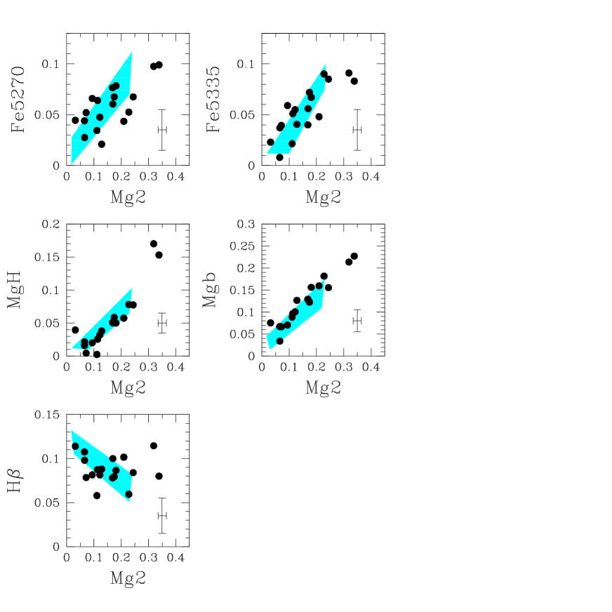
Figure 7: Mg2 versus various other indices, with the range spanned by Milky Way and M31 globular clusters shown as shaded region (taken from Brodie & Huchra 1990 and Burstein et al. 1984). Beside two very metal–rich objects, all globular clusters are consistent with abundances found in the Milky Way and M31 globular clusters

In Fig. 7 we show the relations between Mg2 and various other indices, together with the range covered by the Milky Way and M31 globular clusters (shown as shaded areas).

The first point to note is that the globular clusters in NGC 1399 (except for two clusters that we will discuss further below) cover the entire range spanned by Milky Way and M31 globular clusters. They do not show anomalies in the metal–tracing indices such as Mg and Fe, or in the more age–sensitive index, H$\beta$. Apparently NGC 1399 mostly hosts globular clusters with ages and metallicities similar to those found in the spirals of the Local Group.

In Fig. 8 and 9 we plot Mg2 versus the equivalent width of Fe5270, Fe5335 and H$\beta$ in order to compare them to population synthesis models, to the value of the host galaxy NGC 1399, and to similar plots for elliptical galaxies (e.g Worthey et al. 1992). The indices of Table 2 are shown as solid dots. For clusters #2 and #14 we also included the indices measured in the new Lick/IDS system (new bandpass definitions, resolution degraded to 9 Å) as open circles. The values for NGC 1399 itself are taken from Trager (1997) and shown as triangles. For completeness we show in Table 2 also the line indices derived by Huchra et al. (1996) for NGC 1399. Note that these latter did not deconvolve the galaxy spectrum with the velocity dispersion of the galaxy before measuring the line indices. This leads to systematically lower values of Huchra et al. (1996) and prevents a direct comparison with Trager’s or the globular cluster measurements. In Fig. 8 the population synthesis models of Fritze-v. Alvensleben & Burkert (1995) are shown as long dashed lines for 8 and 16 Gyr year old populations, with metallicity varying between Z=0.001 and Z=0.04. Worthey’s (1994) models are plotted as short dashed lines for 8 and 17 Gyr and metallicity varying between $[$Fe/H$]=-2.0$ and $0.5$ dex. The range covered by the Mg–rich elliptical galaxies of Worthey et al. (1992) is shown as a hatched area. The same symbols are used in Fig. 9, except that we show the tracks for 16, 8, and 3 Gyr for models of Fritze-v. Alvensleben & Burkert (1995), and for 17, 8, 3, and 1.5 Gyr in the case of Worthey’s (1994) models.

4.2.1 Mg2 versus Fe

The observed relations between Fe and Mg2 are well–reproduced by the population synthesis models of Fritze-v. Alvensleben & Burkert (1995) and Worthey (1994). Given the small age dependence of these indices and our errors, we cannot discriminate age differences from this plot (Fig. 8). Worthey et al. (1992) report a Mg versus Fe enhancement for large ellipticals. Unfortunately we have only two globular clusters with Mg high enough to compare them with the affected ellipticals. Given our errors on Fe, these two globular clusters are compatible with the models and also fall in the range covered by the Mg–rich ellipticals. The other element observed to be unusually high in bright ellipticals is NaD. Indeed the two metal–rich clusters, especially #14, have high NaD abundances that could hint to abnormal high values. In summary, both globular cluster #2 and #14 have values close to the ones measured for the stars in NGC 1399.

More data for Mg rich globular clusters are clearly needed to investigate this interesting point: Since globular clusters can be as rich in Mg as large ellipticals, their study might constrain the scenarios responsible for the Mg versus Fe enhancement in large ellipticals. Worthey et al. (1992) summarize the three mechanisms that can be responsible for an enhanced $[$Mg/Fe$]$ ratio in large ellipticals versus normal ratios in smaller ellipticals: i) Different star formation timescale i.e. no time for SNe Ia to dilute the abundance ratios set by the earlier SNe II; ii) Variable/flatter IMF, e.g. in mergers, to produce more SNe II versus SNe Ia; iii) Selective loss mechanisms retaining Mg and expelling Fe in giant ellipticals (this last scenario is rather unlikely as they note). While selecting between these scenarios is difficult on the basis of the properties of the starlight alone, globular clusters might help to settle the issue. If, for example, the Mg enrichment is a result of a flatter IMF for star formation in mergers, globular clusters formed in mergers will show the Mg over–enrichment too. If, however, the high $[$Mg/Fe$]$ values are the result of different star formation timescales among ellipticals, and the Mg–rich globular clusters are young (a possibility discussed below), e.g. formed in a later merger, then they will probably not show the higher $[$Mg/Fe$]$ ratios.

4.2.2 Mg2 versus H$\beta$

The relation between Mg2 and H$\beta$ is interesting in many respects. First it shows the significant differences in the predictions from various models for the value of H$\beta$ at a given age and metallicity. A discussion of the causes of these differences is out of the scope of this paper. We concentrate on the points in common to all models. These are, on the one hand that our globular clusters (except for the two outliers) could span a large range of age according to the models. Our error in H$\beta$ does not allow an age determination better than within a factor two, but our measurements are also consistent with a single age, within the errors. And we note that our values lie in the range spanned by the Milky Way globular clusters (see Fig. 7), that span a small (few Gyr) range in age. The NGC 1399 globular clusters could, therefore, all have similar ages and be as old as the globular clusters in the Milky Way.

On the other hand, we note that the H$\beta$ values for our two metal rich clusters cannot be reproduced by any model, no matter what age or metallicity is assumed. Large values for H$\beta$ were already reported (at lower Mg) in some M31 globular clusters (Burstein et al. 1984, Brodie & Huchra 1991). To check alternative explanations to age for strong H$\beta$ values, Burstein et al. (1984) computed a semi–empirical model to estimate the effects on H$\beta$ and Mg when taking a cluster like 47 Tuc or M71 as starting point (both having stubby, red horizontal branches) and changing the horizontal branch to be blue like that of M5 (so as to yield maximum H$\beta$ strength). Their result shows that H$\beta$ can be raised roughly from 1.5 Å to 2.5 Å, without significantly affecting the Mg abundance. Quantitatively, this alone could explain the position of globular cluster #2 and #14 in Fig. 9. This is very interesting in the light of the extended blue horizontal branches found recently by Rich et al. (1997) in metal rich Milky Way globular clusters. Blue horizontal branches are unexpected (and were, until recently, not observed) at typical bulge metallicities (e.g. Fusi-Pecci et al. 1992, 1993). This is probably the reason why the contribution of a blue horizontal branch is not taken into account in any of the models at high metallicities even though it can contribute to stronger H$\beta$ values. To date, in the models of metal–rich stellar populations, most of the contribution to H$\beta$ and the blue light came from stars from the turn–off region, so that variations in color or H$\beta$ had to be explained by the position of the turn–off point, i.e. by variations in age. This necessarily created a strong age–metallicity degeneracy. New models which include the possible contribution of blue horizontal branches are clearly needed to cover the whole of the possible abundance range at given age and metallicity for globular clusters. More data for globular clusters at high Mg and H$\beta$ might help in the future to fine–tune the populations synthesis models.

4.2.3 The most metal rich clusters

Our two clusters #2 and #14 are outliers in many respects and bring insight into some of the properties of very metal rich globular clusters. Unfortunately we do not have a V$-$I color for our cluster #2 and the B${}_{j}-$R color is too uncertain to rely on (e.g. compare colors for #10 and #20). However, #14 is the reddest cluster in the sample and falls in the very red tail of the color distribution (Kissler-Patig et al. 1997), hinting that such objects are rare. Further these two objects show that globular clusters can have solar abundances (see Table 3) but they are not much in excess of solar (except perhaps for their Mg abundances). This is contrary to results from broad–band photometric studies (Johnson & Washington photometry) in several galaxies (e.g. Secker et al. 1995 for the most extreme case) where globular clusters were reported as having metallicities up to four times solar. While the abundances of the rest of the clusters in NGC 1399 are similar to abundances found in the Milky Way and M31, the abundances of clusters #2 and #14 are clearly anomalous.

We note that the measurement of the H$\beta$ index is controlled in a negative sense by Mg (Tripicco & Bell 1995). Thus, in our particular case, H$\beta$ could even be slightly underestimated. In order to further check the strength of the Hydrogen lines, we measured H$\gamma$ for clusters #2 and #14, using the bandpasses defined by Worthey & Ottaviani (1997) extending the Lick/IDS system (H$\gamma_{A}$ for young stellar populations, H$\gamma_{F}$ for old stellar populations). For this purpose we degraded the resolution of our spectra to 9 Å and re–determined the wavelength calibration around the H$\gamma$ line, before measuring the indices. In both cases we were close to the blue limit of our spectral range in a region showing a factor 10 less signal than in the region between 4800Å and 6000Å. We obtained values of H$\gamma_{A}=-4.0\pm 5.0$ Å and $-3.7\pm 2.0$ Å and H$\gamma_{F}=2.1\pm 2.2$ Å and $-0.5\pm 1.2$ Å for clusters #2 and #14 respectively. Despite the large errors, all the values are unexpectedly high at the high Mg values and are incompatible with high ages ($>8$ Gyr) according to Worthey & Ottaviani (1997). Further, the blue continuum bandpass for H$\gamma$ exactly covers the G–band, which is strong in both clusters, so that our H$\gamma$ indices are probably underestimates when compared to young stellar systems.

It remains unclear how to interpret these strong Balmer lines, and in particular the high H$\beta$ values. As discussed above, they could be explained by the presence of blue horizontal branches (which would also account for the location of the clusters in Fig. 9) and/or the strong Balmer lines could be, at least partly, associated with a younger age but new models would have to be computed for a reliable comparison. A young age cannot, by itself, explain the location of the clusters in Fig. 9. For ages as young as 1 to 5 Gyr, one would expect diluted metal lines and blue broad–band colors, which are definitively not seen in these clusters. However, a younger age would be consistent with the very high metallicities of these clusters (see next section) in a picture where they formed later than the other clusters from highly enriched gas.

Their absolute luminosities provide no further clues. The difference between an 15 Gyr and 2 Gyr old cluster (same mass and same metallicity) would be on the order of 2 magnitudes. These clusters are not exceptionally luminous within our sample. They have absolute V luminosities around $-10.3$ given our assumed distance. They could be old and have masses as high as Omega Centauri (V$=-10.16$, the most massive globular cluster in the Milky Way) or be younger and have lower, more “normal”, masses.

Finally, we note that three of our other globular clusters show Mg values at the upper limit of the range spanned by the Milky Way and M31. Two of these clusters also exhibit slightly stronger H$\beta$ values, than expected for old clusters (although not significantly when considering the errors). This might be yet another sub–population. Clearly, larger samples of globular clusters with well–defined abundances will be valuable in exploring in more detail globular cluster systems with complex formation histories.

4.3 Deriving metallicities

We derived $[$Fe/H$]$ values for the globular clusters using our indices and following the method of Brodie & Huchra (1990). We applied their index–$[$Fe/H$]$ relations to various elements and listed the results in Table 3. We include values for the G–band, CN, and the Ca H$+$K lines for the few spectra extending far enough to the blue, as well as NaD where the night sky lines could be well enough subtracted. Brodie & Huchra (1990) derived the relations from Milky Way and M31 clusters, i.e. the relations do not extend to the high metallicities seen for some of the globular clusters in NGC 1399. In particular, we found the relations between Mg2 and $[$Fe/H$]$, as well as between MgH and $[$Fe/H$]$ to be badly approximated by a linear extrapolation at higher metallicities (Mg2$>0.180$) when compared to population synthesis models (see Fig. 10). For these two relations we applied a correction to the five and two most metal–rich globular clusters respectively by allocating them the metallicity predicted by the 17 Gyr models at their Mg abundance. In addition to the $[$Fe/H$]$ values from individual indices we computed a mean $[$Fe/H$]$ value from Fe5270 and Mg2 (shown in column 10 of Table 3) and a weighted mean $[$Fe/H$]$ from all available indices (column 11). The weights were chosen to reflect the quality of the calibrating relation on the one hand, and the quality of the measured index on the other hand. We assigned weights of 1 to Mg2 and Fe5270, and 0.2 to all other available indices. We estimated the errors from the errors on the indices. The error on the final weighted mean metallicity is estimated to be 0.20 dex for most clusters, slightly higher ($\simeq 0.30$ dex) for the clusters with high Mg2.

Brodie & Huchra (1990) calibrated their index–metallicity relations using the metallicities from Zinn & West (1984), which are mainly based on the Ca II K line. The Zinn & West scale was recently claimed to be slightly non–linear compared to the total metal abundance scale (Carreta & Gratton 1997). We emphasize that our results are necessarily tied, via the Brodie & Huchra (1990) calibration, to the Zinn & West (1984) results.

In Fig. 11 we plotted $[$Fe/H$]$ values derived from Fe5270 and Mg2 versus each other and versus the weighted mean $[$Fe/H$]$ values. We also show a histogram over the weighted mean metallicity values for our clusters. The $[$Fe/H$]$ values derived from Mg for high metallicities lie somewhat above the values derived from Fe5270. As already mentioned, this is mostly due to the fact that, for these high Mg2 values, the relation defined by Brodie & Huchra (1991) is no longer valid, and our correction crude. It could also be due to a slight over–enrichment of Mg versus Fe, but our data do not allow us to make any strong statement in this regard (see last section). In Fig. 11 (lower left panel), three additional clusters seem to have deviating Mg/Fe ratios, however this trend is not confirmed by their Fe5335 values in Fig. 8 (lower panel) where these clusters show normal Fe5335 versus Mg2 abundances. For metallicities below -0.3 dex the agreement between the $[$Fe/H$]$ value derived from Mg2 and Fe5270 is good.

The histogram over the weighted mean $[$Fe/H$]$ values shows that our sample includes globular clusters with metallicities ranging from typical values for Milky Way halo globular clusters to slightly above solar but there are no objects with significantly super–solar abundances. Very metal poor clusters ($[$Fe/H$]<-1.6$) appear to be missing, but recall that the blue part of the globular color distribution in NGC 1399 is not well–sampled. The mean metallicity for our sample is $[$Fe/H$]=-0.83\pm 0.13$ dex (the error is the standard error of the mean). The prediction from the galaxy luminosity – mean globular cluster metallicity relation of Brodie & Huchra (1991) is $[$Fe/H$]=-1.14\pm 0.12$, or $[$Fe/H$]=-0.91\pm 0.16$ (when using the relation defined from ellipticals only), adopting, for NGC 1399, B${}_{\rm T}=10.55$ mag (de Vaucouleurs et al. 1991) and a distance modulus of 31.43 (Madore et al. 1997).

Because of the size of our spectroscopic sample, we have to return to broad–band colors to comment further on the metallicity distribution in the globular cluster system of NGC 1399.

5 Broad–band colors versus indices and metallicity

In this section we compare the line indices with the broad–band colors of our globular clusters. We present the indices versus our V$-$I colors from Kissler-Patig et al. (1997), for which the typical error on the color is 0.035 mag at these magnitudes. Being of photographic origin, the uncertainties in existing B${}_{j}-$R colors (from Grillmair 1992) listed in Table 1 are too large (of the order of 0.3 mag) for our purposes.

In Fig. 12 we show our V$-$I colors versus Mg2, Mgb, $<$Fe$>$ (defined as the mean of Fe5270 and Fe5335, as introduced by Burstein et al. 1984), and H$\beta$. We note that the broad–band color correlates well with the metal indices. This might have been expected since neither Mg or Fe are very age sensitive (e.g. Worthey 1994), so that age–metallicity degeneracy is not a factor here. However, we note that V$-$I also correlates well (inversely) with H$\beta$. As in Fig. 9, the V$-$I colors scatter by less than their typical errors, and are therefore consistent with a single age for these clusters. But, as already noted above, the limiting factor in deriving ages are our errors in H$\beta$ which span a factor of two in age according to population synthesis models (e.g. Fritze-v. Alvensleben & Burkert 1995, Worthey 1994).

Formal linear fits return the following relations:
Mg2 $=-0.46(\pm 0.09)+0.57(\pm 0.08)$V$-$I
$<$Fe$>$ $=-0.08(\pm 0.02)+0.12(\pm 0.02)$V$-$I
H$\beta=0.17(\pm 0.03)-0.07(\pm 0.03)$V$-$I

In Fig. 13 we plot our V$-$I colors versus the weighted mean [Fe/H] (see above section and Table 3) as filled triangles, together with the values for all Milky Way globular clusters that have a reddening of less than E(B$-$V)=0.2 (open circles). The Milky Way values were taken from the McMaster database (Harris 1996) and de–reddened according to Rieke & Lebofsky (1985). For our cluster #14 we plotted the metallicity derived from Fe5270, as an open triangle. For the first time, insight can be gained into the relationship between globular cluster metallicities and colors for the reddest clusters (V$-$I $>1.1$ mag).

We note that the relation may be slightly non–linear in the sense that the slope gets flatter to redder colors, as predicted by the population synthesis models. While the V$-$I color reflects well metallicity, as shown above, it could still be affected by age within our errors. We stress again that the ages of our globular clusters are not well defined, but they are compatible with the ages of Milky Way globular clusters, as inferred from all the measured element abundances. The most metal–rich globular clusters may have formed later than the rest. If they are, for example, half as old as the metal poor ones, their V$-$I color is shifted to the blue by 0.1 magnitude. That is, if we corrected the colors of our most metal rich globular clusters for age, we would get an even flatter slope. However since the ages are uncertain, we will not apply any corrections for age to the colors in what follows.

Given the restricted number of data points for colors above V$-$I=1.2, we attempted only a linear fit to the sample (including the selected Milky Way globular clusters). The returned relation between metallicity and V$-$I is:

$[$Fe/H$]$ $=-4.50(\pm 0.30)+3.27(\pm 0.32)$V$-$I

The slope of this relation is almost twice as flat as the ones previously derived by Couture et al. (1990) and Kissler-Patig et al. (1997) from the Milky Way globular clusters alone. A non–linear fit will lead to an even more dramatic result. For red colors, metallicities derived from V$-$I, and most probably from other broad–band colors too, have been overestimated. Since most globular cluster systems in early–type galaxies have red median colors (V$-$I $>1.1$), most mean metallicities have probably been overestimated in the past.

Kissler-Patig et al. (1997) have shown that the color distribution of NGC 1399 has two “peaks” at V$-$I $=0.99$ mag and V$-$I $=1.18$ mag (confirming the multi–modal distribution found with Washington photometry by Ostrov et al. 1993, also seen by Forbes et al. 1997). Thus, if these two peaks are associated with two different sub–populations, these two populations would have mean metallicities around [Fe/H]$=-1.3$ dex and [Fe/H]$=-0.6$ dex, very similar to the means of the halo and disk/bulge populations of the Milky Way. The same applies to globular clusters in M87 which peak at V$-$I$=0.92$ and V$-$I$=1.23$ (Elson & Santiago 1996). This corresponds to [Fe/H]$=-1.5$ dex and [Fe/H]$=-0.5$ dex, similar to NGC 1399 and again similar to the Milky Way. Further, the small ellipticals NGC 1374, NGC 1379, NGC 1387, NGC 1427 which appear uni–modal (Kissler-Patig et al. 1997) would have mean metallicities around [Fe/H]$=-0.9$, $-0.7$, $-0.6$, $-1.1$ dex respectively. That is, their globular clusters do not have solar or super–solar mean abundances as previously thought. Moreover, the spread in metallicity between the different galaxies is reduced to 0.5 dex instead of 1 dex, leading to a more homogeneous picture and smaller discrepancies between metal–rich globular clusters in spirals and ellipticals.

Finally we note that very metal–rich globular clusters such as our objects #2 and #14, with V$-$I colors $\geq 1.35$ make up only a small fraction (2–5%) of the total globular cluster system, as derived from the color distribution of Kissler-Patig et al. (1997). If these objects are significantly younger, i.e. brighter, they might even be over–represented in the magnitude limited sample of Kissler-Patig et al. (1997) and represent an even smaller fraction of the total globular cluster system.

We conclude from the above that V$-$I, and thus probably the other broad–band colors too, trace metallicity relatively well in globular cluster systems. Drawing a tentative conclusion from this sample, the V$-$I relation can be used if most objects are old and do not show a significant age spread, as it seems the case for our sample that scatters around an isochrone within the measurement errors (see section 4). Generally, this will be the case for any globular cluster system that formed at high redshift with no significant fraction of clusters that formed since $z\simeq 1$. Further, given the spread in [Fe/H] at a given color, metallicities from V$-$I will be accurate only to 0.5 dex for individual objects. However, mean metallicities for entire globular cluster systems can probably be derived with an accuracy of 0.3 dex from V$-$I. This will, for example, allow corrections for metallicity effects to distances derived from the globular cluster luminosity function, when the mean color of the globular cluster system is known, as proposed by Ashman, Conti & Zepf (1995).

6 Discussion

Most globular clusters in NGC 1399 have very similar Mg, Fe and H$\beta$ line indices to the Milky Way and M31 globular clusters and span the full range observed in these galaxies. The metal–poor clusters have metallicities corresponding to the mean metallicity of Milky Way halo clusters, the metal–rich clusters have similar metallicities to Milky Way bulge/disk clusters. Their Mg and Fe and especially H$\beta$ indices indicate that these clusters are probably as old as the Milky Way globular clusters, although deriving accurate ages is difficult given the observational errors and model uncertainties.

Two clusters clearly stand out in their abundances. They have Mg and Fe (and Na) indices significantly higher than observed in any globular cluster in the Milky Way or M31, and comparable to the integrated starlight of giant ellipticals. Their metallicities are estimated to be around, or even slightly above, solar. Whether or not these clusters exhibit a Mg versus Fe over–abundance, as seen in the integrated starlight of giant ellipticals, remains an interesting open question. Moreover, these two clusters show abnormally high H$\beta$ (and H$\gamma$) values that cannot be matched by population synthesis models for any age and metallicity, making any age determination very uncertain and calling for an explanation. Blue horizontal branches in these metal–rich clusters would qualitatively be a solution. The formation of these globular clusters several gigayears after the more metal–poor globular clusters could also be part of the explanation but needs revisited models including blue horizontal branches at high metallicity for comparison. This would confirm the formation of at least some globular clusters in a later phase as suggested for globular clusters forming in mergers (Schweizer 1987, Ashman & Zepf 1992). From the globular cluster color distribution, we estimate that these peculiar clusters do not make up more than 5% of the total population, hinting to mergers involving little dissipation.

The overall picture of the system seems to hint at the presence of various sub–populations similar to the ones seen in the Milky Way, as well as a small fraction of globular clusters that formed later from highly enriched gas. That is, processes like the ones that produced the Milky Way halo and disk/bulge population can be responsible for the formation of the vast majority of the globular clusters in NGC 1399, only a small percentage of the total number of globular clusters need to have formed later from solar metallicity gas. Fritze-v. Alvensleben & Gerhard (1994) showed that, at the end of a starburst induced by a merger event, the metallicity can reach solar, independently of the age of the event (under the assumption that no gas is lost from, or accreted by, the merging galaxy pair). This would allow the formation of the extremely metal–rich clusters in a merger as soon as 3 Gyr after the formation of the progenitor galaxies if globular clusters formed at the end of the starburst. These few new globular clusters would be added to the globular clusters already present in the progenitors (the majority).

Translated into implications for the formation of NGC 1399 and its over–abundant globular cluster system: The galaxy and its globular clusters are likely to have formed at an early time. The blue population formed from material as metal poor as the Galactic halo, despite the fact that it existed in a high density environment like the center of a cluster of galaxies, and it presumably formed at a similar early epoch. The relatively low mean metallicity (compared to previous estimates, based on broad–band colors) of the “red” population (peaking at V$-$I=1.18) of $[$Fe/H$]\simeq-0.6$ dex, implies formation before the gas could be enriched to solar abundances. Whether these globular clusters formed in early merger events or during the collapse of the “bulge” (as might have been the case in the Milky Way, e.g. Minniti 1995) cannot be distinguished from our data. However, judging by the globular cluster color distribution and the metallicity of the very red objects, only a very small fraction of the globular clusters clearly formed later from solar metallicity gas, i.e. later mergers are unlikely to be the cause for the over–abundant globular cluster system of NGC 1399. To explain the abnormally high number of globular clusters and specific frequency of NGC 1399, alternative models are needed (see e.g. Forbes, Brodie & Grillmair 1997, Blakeslee et al. 1997), and the role of mechanisms like stripping from neighboring galaxies (Muzzio 1987), or accretion of dwarf galaxies (Hilker et al. 1997) must be better understood.

7 Summary and Conclusions

We obtained moderate resolution spectra for 18 globular clusters in the giant elliptical cD galaxy NGC 1399 in Fornax. From the derived velocities we calculated a galaxy mass of 1 to $5\times 10^{12}M_{\odot}$, leading to a mass to light ratio of $M/L_{\rm B}=36\pm 20$ or $76\pm 40M_{\odot}/L_{\odot}$ (depending on the estimator) within 5 arcmin (6.7 r_eff), for an assumed distance of 19.3 Mpc. This would imply a dark matter dominated potential at this radius. No correlation between magnitude, color or position with velocity could be found in our small sample.

The element abundances of most globular clusters in NGC 1399 do not differ from the ones observed in the Milky Way and M31. No different processes and formation time than the ones assumed for the formation of the Milky Way halo and disk/bulge globular clusters are needed to explain the majority of globular clusters in NGC 1399. However, two of the globular clusters in our sample clearly stand out in the strength of their line indices and show abundances similar to the starlight of giant ellipticals. They must have formed from solar metallicity gas in a different formation process, e.g. merger event, although not necessarily much ($>3$ Gyr) later than the others. Further, these very metal rich clusters show unexplained high H$\beta$ (and H$\gamma$) abundances, incompatible with any age–metallicity combination of existing models. These abundances can, however, be explained by blue horizontal branches. Judged from the color distribution, these clusters represent less than 5% of the total number of globular clusters. This hint at late mergers not being the cause of the over–abundant globular cluster system around NGC 1399.

The age–metallicity degeneracy of broad–band colors, as predicted by the models, is presumably artificially strengthen by not taking into account a possible contribution to the blue light from the horizontal branch at high metallicities. Broad–band colors turned out to be very good metallicity tracers in the globular cluster system. While for individual cases the metallicity of a globular cluster can only be derived to an accuracy of 0.5 dex from its V$-$I color, the mean metallicity of a globular cluster system can be determined to an accuracy of about 0.3 dex. However, we stress that the relation derived here has a slope about twice as shallow as the ones previously extrapolated from the Milky Way system, making globular cluster metallicity differences between galaxies less significant and bringing estimates for red globular clusters back from super–solar to solar metallicities.

These conclusions were drawn from a sample of only 18 globular clusters. The picture will certainly improve as more spectroscopic studies from 10–m class telescopes appear in the future.

In a recently submitted paper Cohen, Blakeslee & Ryzhov (1998) present a similar study in M87. They obtained Keck/LRIS spectra for a larger sample of globular clusters and find a similar metallicity range as for the clusters in NGC 1399, ranging from metal–poor to solar metallicities, and an old median age for their globular cluster sample. Their spectroscopy strengthen the point that globular clusters in large ellipticals have very similar line indices to the globular clusters in the Milky Way and M31.

Table 1: List of our candidate globular clusters around NGC 1399

ID	RA(1950)	DEC(1950)	V   (a)	V$-$I   (a)	$B_{j}$   (b)	$B_{j}-R$   (b)	$v_{\rm helio}$	$v_{G+94}$(c)
			$\pm 0.02$	$\pm 0.035$	$\pm 0.2$	$\pm 0.3$
1	3 36 13.8	-35 39 24.8			21.8		732 $\pm 32$
2	3 36 14.2	-35 38 51.2			22.4	1.19	1094 $\pm 34$
3	3 36 09.4	-35 37 32.4			22.3	1.02	1571 $\pm 31$
4	3 36 12.0	-35 37 44.3			21.9	1.20	279 $\pm 72$
5	3 36 13.2	-35 37 37.8			21.8	1.17	1775 $\pm 66$
6	3 36 17.8	-35 37 50.2			22.3		1386 $\pm 31$
7	3 36 16.7	-35 37 01.7	21.01	1.23	21.7	1.31	1376 $\pm 84$	1677 $\pm 150$
8	3 36 15.4	-35 36 17.1			22.3	1.34	$z\simeq 0.31$
9	3 36 19.2	-35 36 28.7	21.04	1.25	21.8	1.33	1150 $\pm 31$	1280 $\pm 150$
10	3 36 21.5	-35 36 04.4	20.55	1.05	21.4	1.50	815 $\pm 30$	980 $\pm 150$
11	3 36 25.0	-35 36 28.3	21.34	1.17	22.2	1.50	1338 $\pm 33$
12	3 36 20.3	-35 35 15.3	21.97	0.94	22.4	1.06	1736 $\pm 31$	1701 $\pm 150$
13	3 36 23.4	-35 35 37.2	21.51	0.91	22.2		1247 $\pm 30$
14	3 36 24.5	-35 35 36.8	21.17	1.37	22.1	1.65	1260 $\pm 66$
15	3 36 23.2	-35 34 39.3	21.26	1.04	22.0	1.26	1523 $\pm 30$
16	3 36 25.0	-35 34 31.5			22.1	1.56	$z\simeq 0.27$
17	3 36 26.3	-35 34 20.7	21.55	1.14	22.4	1.33	866 $\pm 71$
18	3 36 31.4	-35 35 05.9	21.32	1.08	22.3	1.50	1688 $\pm 42$
19	3 36 34.5	-35 34 52.2	21.41	1.29	22.3		1150 $\pm 59$
20	3 36 28.5	-35 33 17.0	21.63	1.13	22.3	0.88	1374 $\pm 126$
21	3 36 35.7	-35 34 24.6	21.15	1.09	22.0	1.37	1194 $\pm 98$	1062 $\pm 150$
NGC 1399 (d)	3 36 34.4	-35 36 45.0	9.59	1.25			1447 $\pm 12$

c r r r r r r r r r 2 Measured indices for the globular clusters ID & Mg2 MgH Mgb Fe5270 Fe5335 H$\beta$ Gband NaD TiO
$\pm 0.015$ $\pm 0.015$ $\pm 0.025$ $\pm 0.020$ $\pm 0.020$ $\pm 0.020$ $\pm 0.045$ $\pm 0.030$ $\pm 0.030$
1 & 0.072 0.005 0.067 0.052 0.040 0.079
2 0.319 0.170 0.214 0.098 0.091 0.115 0.154 0.030
3 0.111 0.003 0.089 0.035 0.022 0.058 0.060
5 0.094 0.020 0.071 0.066 0.059 0.082 0.096 0.042 0.033
6 0.129 0.038 0.127 0.021 0.041 0.088 0.026
7 0.228 0.078 0.182 0.053 0.090 0.060 0.114 0.174 0.028
9 0.174 0.059 0.123 0.068 0.072 0.080 0.136 0.063 0.027
10 0.066 0.022 0.034 0.028 0.037 0.098 0.081 0.017
11 0.179 0.051 0.129 0.061 0.056 0.100 0.029
12 0.032 0.040 0.076 0.045 0.023 0.114 0.079 0.065
13 0.066 0.016 0.067 0.044 0.008 0.108 0.096 0.017
14 0.339 0.153 0.227 0.099 0.083 0.080 0.283 0.034
15 0.114 0.026 0.097 0.064 0.051 0.088 0.103 0.023
17 0.210 0.058 0.160 0.044 0.048 0.102 0.169 0.071 0.036
18 0.181 0.050 0.156 0.079 0.067 0.087 0.039
19 0.244 0.078 0.156 0.068 0.085 0.084 0.168 0.062
20 0.122 0.032 0.101 0.048 0.055 0.082 0.048
21 0.168 0.051 0.129 0.077 0.040 0.078 0.182 0.055

NGC 1399 (a) 0.371 0.201 0.202 0.081 0.082 0.052 0.197 0.261 0.059
$\pm 0.008$ $\pm 0.007$ $\pm 0.012$ $\pm 0.007$ $\pm 0.014$ $\pm 0.013$ $\pm 0.039$ $\pm 0.013$ $\pm 0.007$
NGC 1399 (b) 0.288 0.186 0.113 0.038 0.045 0.223 0.122
$\pm 0.024$ $\pm 0.021$ $\pm 0.040$ $\pm 0.029$ $\pm 0.037$ $\pm 0.052$ $\pm 0.038$
All bandpass definition were taken from Brodie & Huchra (1990) (a)Taken from Trager (1997) (b)Taken from Huchra et al. (1996), note that, contrary to Trager’s data, the measurements were made on the galaxy spectra without correcting for velocity dispersion, and can therefore not be directly compared with them or the globular cluster measurements

c rrrrrrrr cc 3 $[$Fe/H$]$ calculated from various line indices for the globular clusters ID & Mg2 Fe5270 MgH Mgb Gband NaD CN H+K mean from weighted
Mg2 Fe5270(a) mean(a)
$\pm 0.15$ $\pm 0.35$ $\pm 0.30$ $\pm 0.35$ $\pm 0.50$ $\pm 0.40$ $\pm 0.50$ $\pm 0.50$ $\pm 0.20$ $\pm 0.20$
1 &-1.51 -1.04 -1.74 -1.27 -1.19 -1.27 -1.30
2 0.18 -0.10 0.41 0.80 -0.14 0.04 0.12
3 -1.11 -1.37 -1.78 -0.96 -1.76 -1.17 -1.24 -1.29
5 -1.28 -0.75 -1.42 -1.21 -1.36-1.75 -0.95 -1.13 -1.01 -1.12
6 -0.94 -1.65 -1.05 -0.42 -1.29 -1.20
7 -0.27 -1.01 -0.23 0.35 -1.16 0.15 -1.03 -0.64 -0.55
9 -0.48 -0.71 -0.63 -0.49 -0.90 -0.45 -0.59 -0.60
10 -1.56 -1.52 -1.40 -1.74 -1.53 -1.35 -1.54 -1.53
11 -0.53 -0.85 -0.79 -0.4 -0.69 -0.67
12 -1.90 -1.18 -1.03 -1.13 -1.55-1.43 -1.54 -1.47
13 -1.56 -1.19 -1.51 -1.26 -1.35 -1.42 -1.24 -1.37 -1.37
14 0.26 -0.08 0.26 0.99 1.72 0.09 0.30
15 -1.09 -0.78 -1.30 -0.85 -1.28 -0.93 -0.98
17 -0.38 -1.21 -0.65 0.04 -0.52 -1.33 -0.73 -0.89 -0.79 -0.81
18 -0.42 -0.50 -0.81 -0.01 -0.46 -0.45
19 -0.17 -0.72 -0.25 -0.02 0.07 -0.40 -0.32
20 -1.00 -1.12 -1.19 -0.79 -0.99 -1.06 -1.04
21 -0.54 -0.53 -0.79 -0.38 -0.39 -0.54 -0.54

NGC 1399 (b) 0.52 -0.44 0.85 1.19 -0.21 1.41 0.04 0.26
All [Fe/H] values were calculated using the index–metallicity relations of Brodie & Huchra (1990) (a) The last two columns list the arithmetic mean of the metallicity derived from Mg2 and Fe5370 and a weighted mean (see text for assigned weights) respectively (b)calculated from the values in Table 2

Figure 1: Comparison between velocities derived in this work and in Grillmair et al. (1994) for the five globular clusters in common to both samples

Figure 2: Position of approaching (open) and receding (solid) globular clusters (reference velocity is 1293 km/s), the rings mark 1 and 5 r_eff around NGC 1399

Figure 3: Velocity distribution of our 18 globular clusters around NGC 1399. The dashed line marks the radial velocity of the stellar component (de Vaucouleurs et al. 1991)

Figure 4: Velocities versus V magnitudes and V$-$I colors of the globular clusters. No trend can be seen in our sample

Figure 5: Velocities versus radius (in arcmin) for the globular clusters. The dashed line marks the radial velocity of the stellar component (taken from de Vaucouleurs et al. 1991). No trend can be seen in our sample

Figure 6: Three representative spectra, ranging from blue, over red, to very red color. The spectra were smoothed over 3 pixels. While the H$\beta$ gets slightly weaker from the blue to the red object, the metal lines (Mg, Fe, Na) become much stronger

Figure 8: Mg2 versus the equivalent width of Fe5270 and Fe5335. Tracks for 8 and 16 Gyr old stellar populations (metallicity varying between Z=0.001 and Z=0.04) from Fritze-v. Alvensleben & Burkert (1995) are plotted as long dashed lines, tracks for 8 and 17 Gyr old stellar populations (metallicity varying between $[$Fe/H$]=-2.0$ and $0.5$ dex) from Worthey (1994) are plotted as short dashed lines. The regions spanned by elliptical galaxies in Worthey et al. (1992) are lined. NGC 1399 (taken from Trager 1997) is plotted as a triangle. Open circles are measurements using the updated Lick/IDS bandpasses on artificially degraded spectra (see text)

Figure 9: H$\beta$ (here in Å) versus Mg2 with tracks from Fritze-v. Alvensleben & Burkert (1995) (long dashed lines, metallicity varying between Z=0.001 and Z=0.04) and from Worthey (1994) (short dashed lines, metallicity varying between $[$Fe/H$]=-2.0$ and $0.5$ dex). Other symbols as in Fig. 8

Figure 10: Comparison between the metallicities derived from Mg2, MgH, Mgb and Fe5270 using the relation of Brodie & Huchra (1990) (solid line), and the values predicted by the models of Worthey (1994) (dashed lines). The solid dots show our data points, when using the Brodie & Huchra (1990) relation. The open dots show our data points once corrected for the non–linear behaviour of Mg at high metallicities. We corrected five values derived from Mg2, two derived from MgH. Values derived from Mgb or Fe5270 do not need any corrections.

Figure 11: Comparison between the metallicities derived from Mg2, Fe5270, and mean metallicity as defined in the text. The lower right panel shows a histogram over the mean metallicities of the globular clusters

Figure 12: V$-$I colors of the globular clusters versus Mg, Fe and H$\beta$. The broad–band color correlates well both with the metal and (inverse) Hydrogen abundance

Figure 13: V$-$I color versus mean metallicity of the globular clusters in NGC 1399 (triangles), for cluster #14 the metallicity from Fe5270 alone is also shown (open triangle). Over–plotted as open circles are all Milky Way globular clusters with E(B$-$V)$<0.2$ (taken from Harris 1996, de–reddened according to Rieke & Lebofsky 1985). The solid line is the best fit to the data, the dashed line was derived from the Milky Way sample by Kissler-Patig et al. (1997) and extrapolated to higher metallicities