Statistical Properties of X-ray Clusters: Analytic and Numerical Comparisons

Abstract

We compare the results of Eulerian hydrodynamic simulations of cluster formation against virial scaling relations between four bulk quantities: the cluster mass, the dark matter velocity dispersion, the gas temperature and the cluster luminosity. The comparison is made for a large number of clusters at a range of redshifts in three different cosmological models (CHDM, CDM and OCDM). We find that the analytic formulae provide a good description of the relations between three of the four numerical quantities. The fourth (luminosity) also agrees once we introduce a procedure to correct for the fixed numerical resolution. We also compute the normalizations for the virial relations and compare extensively to the existing literature, finding remarkably good agreement. The Press-Schechter prescription is calibrated with the simulations, again finding results consistent with other authors. We also examine related issues such as the size of the scatter in the virial relations, the effect of metallicity with a fixed pass-band, and the structure of the halos. All of this is done in order to establish a firm groundwork for the use of clusters as cosmological probes. Implications for the models are briefly discussed.

Bryan & Norman Statistical Properties of X-ray Clusters

and

1 Introduction

The statistics of X-ray clusters can serve as an excellent probe of cosmology. The luminosity function of clusters is defined in a straightforward manner both observationally ([Henry et al. 1992]; [Ebeling et al. 1995]; [Burns et al. 1996]) and numerically ([Cen 1992]; [Bryan et al. 1994b]), although as we shall see this is a computationally difficult task. The temperature function is similarly obtainable ([Henry & Arnaud 1991]; [David et al. 1993]), however, here it is the observational data which are more challenging to obtain.

One uncertainty in performing this comparison is the possibility of systematic errors in the theoretically derived cluster temperatures and luminosities. This has been investigated in a number of ways, primarily by testing individual methods developed against simplified problems with known solutions. So, the Lagrangian smoothed particle hydrodynamics (SPH) method combined with a P³M code for computing the gravitational interaction has been examined by Evrard (1988)evr88, Couchman, Thomas & Pearce (1995)cou95 and others; while SPH with a gravitational tree code has been tested in a number of papers ([Hernquist & Katz 1989]; [Katz, Weinberg & Hernquist 1996]; [Navarro & White 1993]). A novel modification of SPH was described by Shapiro et al. (1996)sha96, along with a number of comparisons against known results. For Eulerian codes, method papers with some tests include: Cen (1992)cen92 for a first-order grid based code; Ryu et al. (1993)ryu93 for a total variation diminishing method; Anninos, Norman & Clarke (1994)ann94 for a two-level nested grid scheme, and Bryan et al. (1995)PPM for a code based on the piecewise parabolic method.

However, a number of recent papers have taken up the question of accuracy and consistency with a cosmological context as their primary focus. For Eulerian codes (with fixed comoving spatial resolution), this issue has been addressed by Anninos & Norman (1996)ann96 (hereafter AN96) who performed simulations with a two level hierarchical method and simulated the formation of a moderately rich cluster with five different resolutions ranging from 1600 to 100 kpc per cell. They found that although the temperature, mass and velocity dispersion of a cluster were reasonably well determined with the lower-resolution simulations, the total luminosity had not converged even for the highest resolution run. The bolometric luminosity (for this single cluster) behaved as

$$L_{tot}\propto\frac{1}{\Delta r^{\alpha}},$$ (1)

where $\Delta r$ is the spatial resolution of the simulation and $\alpha=1.17$.

Another way to check the results of simulations (and the route taken in this paper) is to compare them against the predictions of approximate analytic models. Although agreement does not guarantee correctness (as both methods are only approximations to the full solution), concordance would increase our confidence in both methods. Also, simple analytic arguments may only identify a scaling property between quantities without specifying a normalization, which can however, be fixed by numerical simulation (or by further assumptions). This describes the scaling laws that come from considering clusters as spherical clouds of gas in hydrostatic equilibrium. Navarro, Frenk & White (1995)NFW (hereafter NFW) recently compared the results of six clusters simulated with SPH in a Cold Dark Matter (CDM) scenario against these scaling relations (at $z=0$). They find good agreement over a wide range of luminosity, mass and temperature, but claim that clusters from Eulerian simulations (such as in [Kang et al. 1994a] and [Bryan et al. 1994a]) do not.

Another analytic method is that initially described by Press & Schechter (1974)pre74 which predicts the mass distribution of collapsed objects. There have been a number of comparisons between its predictions and the results of N-body simulations ([Efstathiou et al. 1988]; [Bond et al. 1991]; [Lacey & Cole 1996]). Using the scaling results, this theory can be extended to produce the temperature ([Eke, Cole & Frenk 1996]) and luminosity distribution functions. Since this is one of the most widely used constraints on the amplitude of mass fluctuations, it is important to check its validity.

In this paper, we make a detailed comparison between simulation results and the adiabatic scaling laws as well as the Press-Schechter formalism with extensions. This allows us to gauge the accuracy and consistency of both methods, leading to firmer conclusions regarding the viability of the cosmology modelled. The paper is laid out as follows. In section 2, we review the scaling relations, including a modification to take into account the finite resolution of Eulerian codes. We then compare these to the results of CDM and Cold plus Hot Dark Matter (CHDM) simulations at a variety of redshifts. In section 3, we examine the mass, temperature and luminosity distribution functions, including the effects of finite band-pass and line emission. These are compared against the Press-Schechter plus scaling theory (extended to include the additional complications in the luminosity function). In section 4 we briefly examine the profiles of temperature and velocity dispersion to assess the accuracy of the isothermal models assumed in extending the Press-Schechter work. Finally, in section 5, we discuss our results and comment on the viability of the models simulated.

2 Scaling Relations

Here we review the scaling relations between cluster bulk properties through the assumption of a pressure supported isothermal sphere for both the gas temperature $T$ and one-dimensional collisionless velocity dispersion $\sigma$ of the dark matter particles. The assumption of a specific density profile (here the isothermal sphere) is not required to obtain the scaling behaviour, but is needed to determine the constant of proportionality between the given quantities.

These relations were used by Kaiser (1986)kai86 to describe the evolution of ‘characteristic’ quantities, largely driven by the non-linear mass ($M_{nl}$), defined via equation (19) below, as well as to derive relations between distribution functions at different epochs. We do not explicitly test these because they are uniquely specified by the non-linear mass (which we do examine) and the scaling relations discussed below.

2.1 Scaling review and normalization

In the isothermal distribution function, the density is related to the velocity dispersion ([Binney & Tremaine 1987]):

$$\rho(r)=\frac{\sigma^{2}}{2\pi Gr^{2}}.$$ (2)

If we define $r_{vir}$ as the radius of a spherical volume within which the mean density is $\Delta_{c}$ times the critical density at that redshift ($M=4\pi r_{vir}^{3}\rho_{crit}\Delta_{c}/3$), then there is a relation between the virial mass and the one-dimensional velocity dispersion:

$$\sigma = M^{1/3}\left(H^{2}(z)\Delta_{c}G^{2}/16\right)^{1/6}$$ (3)

$$= 476f_{\sigma}\left(\frac{M}{10^{15}M_{\odot}}\right)^{1/3}\left(h^{2}\Delta_{c}E^{2}\right)^{1/6}\hbox{km/s}$$ (4)

In the second line we have introduced a factor $f_{\sigma}$ which will be used to match the normalization from the simulations. The redshift-dependent Hubble constant can be written as $H(z)=100$ $h$ $E(z)$ km/s/Mpc with the function $E^{2}=\Omega_{0}(1+z)^{3}+\Omega_{R}(1+z)^{2}+\Omega_{\Lambda}$ dependent on three contributions:

$$\Omega_{0}=\frac{8\pi G\rho_{0}}{3H_{0}^{2}};\quad\Omega_{R}=\frac{1}{(H_{0}R)^{2}};\quad\Omega_{\Lambda}=\frac{\Lambda}{3H_{0}^{2}}.$$ (5)

Here, $\rho_{0}$ is the non-relativistic matter density, $R$ is the radius of curvature and $\Lambda$ is the cosmological constant.

The value of $\Delta_{c}$ is taken from the solution to the collapse of a spherical top-hot perturbation under the assumption that the cluster has just virialized ([Peebles 1980]). Its value is $18\pi^{2}$ for a critical universe but has a dependence on cosmology through the parameter $\Omega(z)=\Omega_{0}(1+z)^{3}/E(z)^{2}$. We have calculated this for the cases $\Omega_{\Lambda}=0$ ([Lacey & Cole 1993]) and $\Omega_{R}=0$ ([Eke, Cole & Frenk 1996]), fitting the results with:

$$\Delta_{c}=18\pi^{2}+82x-39x^{2}\quad\hbox{for}\quad\Omega_{R}=0$$ (6)

$$\Delta_{c}=18\pi^{2}+60x-32x^{2}\quad\hbox{for}\quad\Omega_{\Lambda}=0$$

where $x=\Omega(z)-1$. These are accurate to 1% in the range $\Omega(z)=0.1$-$1$.

If the distribution of the baryonic gas is also isothermal we can define a ratio of the ‘temperature’ of the collisionless material ($T_{\sigma}=\mu m_{p}\sigma^{2}/k)$ to the gas temperature:

$$\beta=\frac{\mu m_{p}\sigma^{2}}{kT}.$$ (7)

We take $\mu=0.59$. Given equations (3) and (7), the relation between temperature and mass is:

$$kT = \frac{GM^{2/3}\mu m_{p}}{2\beta}\left(\frac{H^{2}(z)\Delta_{c}}{2G}\right)^{1/3}$$ (8)

$$= 1.39f_{T}\left(\frac{M}{10^{15}M_{\odot}}\right)^{2/3}\left(h^{2}\Delta_{c}E^{2}\right)^{1/3}\hbox{keV}$$ (9)

Since we will test the relations 4, 7 and 9 against the numerical simulations separately, we also add a normalization factor, $f_{T}$, and set $\beta=1$ for this last equation.

We can easily find the scaling behaviour of a cluster’s X-ray luminosity by assuming bolometric Bremsstrahlung emission and ignoring the temperature dependence of the Gaunt factor (e.g. [Spitzer 1978]): $L_{bol}\propto M\rho T^{1/2}$.

We could compute the luminosity by using the isothermal sphere approximation, however this is either infinite, if there is no rollover in density as $r\rightarrow 0$, or we must arbitrarily select a core radius. Instead, we will assume the normalization found by NFW (adjusted slightly to match our definition of the virial mass):

$$L_{bol}=1.3\times 10^{45}\left(\frac{M}{10^{15}M_{\odot}}\right)^{4/3}\\ \left(h^{2}\Delta_{c}E^{2}\right)^{7/6}\left(\frac{\Omega_{b}}{\Omega}\right)^{2}\hbox{erg/s},$$ (10)

To obtain this we have used the redshift dependence of the critical density, the temperature-mass relation and multiplied by the mean baryon fraction.

Other scaling laws can easily be derived from these; we will need one more:

$$L_{bol}=6.8\times 10^{44}\left(\frac{kT/f_{T}}{1.0\hbox{ keV}}\right)^{2}\left(h^{2}\Delta_{c}E^{2}\right)^{1/2}\left(\frac{\Omega_{b}}{\Omega}\right)^{2}\hbox{erg/s}.$$ (11)

We note that cosmology enters these relations only with the combination of parameters $h^{2}\Delta_{c}E(z)^{2}$, which comes from the relation between the cluster’s mass and mean density. The redshift variation comes mostly from $E(z)$ which is equal to $(1+z)^{3/2}$ for an Einstein-de Sitter universe.

2.2 Resolution effects

While we do not expect the first three bulk properties (mass, temperature and velocity dispersion) to be strongly dependent on the numerical resolution, the X-ray emissivity is very sensitive to the density profile of the cluster since it originates primarily from the central region of the cluster. In order to examine the expected luminosity behaviour with resolution, we take the density profile fit from high-resolution N-body simulations found in Navarro, Frenk & White (1996)nav96:

$$\frac{\rho(r)}{\rho_{crit}}=\frac{\delta_{0}/c^{3}}{x(1/c+x)^{2}},$$ (12)

where $x=r/r_{vir}$. For clusters, a reasonable parameter choice is $c=5$, although our results will not be sensitive to small changes in this value. This is a fit to the collisionless component and not the baryonic gas (as would be more appropriate), however the difference only becomes important at $r/r_{vir}\leq 0.04$ (c.f. [Navarro, Frenk & White 1995]; [Bryan & Norman 1997a]) which will not substantially affect our results.

In order to approximate the effect of finite numerical resolution we filter the density distribution:

$$\rho^{\prime}(r,r_{sm})=\frac{\int\rho(\vec{r}^{\prime})W_{G}\left(\frac{|\vec{r}^{\prime}-\vec{r}|}{r_{sm}}\right)d^{3}\vec{r}^{\prime}}{\int W_{G}\left(\frac{|\vec{r}^{\prime}-\vec{r}|}{r_{sm}}\right)d^{3}\vec{r}^{\prime}}.$$ (13)

The smoothing kernel is a Gaussian ($W_{G}(x)=e^{-x^{2}/2}$) and $r_{sm}$ is the smoothing radius. Using symmetry, this integral can be partially computed analytically:

$$\rho^{\prime}=\frac{1}{\sqrt{2\pi}rr_{sm}}\int_{0}^{\infty}\rho(r^{\prime})r^{\prime}\left(e^{\frac{-(r^{\prime}-r)^{2}}{2r_{sm}^{2}}}-e^{\frac{-(r^{\prime}+r)^{2}}{2r_{sm}^{2}}}\right)dr^{\prime}.$$ (14)

In Figure 1a, we show the effects of various smoothing radii to the adopted density profile. The mass is conserved by the smoothing process in the sense that the total mass within some fixed fraction $r/r_{sm}\gg 1$ is constant as $r_{sm}$ changes (the total mass of equation (12) does not converge as $r\rightarrow\infty$). This results in mass being transferred from small to large radii, causing the profile to steepen outside the smoothing radius, another feature observed by AN96. Assuming the temperature profile does not change, the bolometric free-free luminosity can be computed as a function of $r_{sm}/r_{vir}$ and the result is shown in Figure 1b. Also shown is the scaling result found by AN96 and given by equation (1), which they found to be approximately valid in the range $0.1>r_{sm}/r_{vir}>1$. The agreement is good enough that we will adopt their value ($\alpha=1.17$), although it should be kept in mind that this power-law behaviour is only approximately correct.

Figure 1: (a) The density profile in equation (12) smoothed by a Gaussian filter with three different values of the smoothing radius. (b) The relative bolometric bremsstrahlung luminosity of the smoothed density profile as a function of smoothing radius. The dashed line shows the result found by direct numerical simulation (AN96).

If all density profiles can be scaled by the virial radius and critical density to agree with equation (12) regardless of mass (at least in a statistical sense), then the smoothed luminosity will scale in general as $L_{bol}\propto(r_{vir}/r_{sm})^{\alpha}$. Recent work ([Navarro, Frenk & White 1996]; [Cole & Lacey 1996]) indicates that, in fact, this is not true and lower mass objects form earlier and have steeper profiles. Nevertheless it is a good approximation over the range of masses examined here and we will adopt it.

Using the relation between the virial radius and virial mass, we can include the effects of numerical resolution in equation (10):

$$L^{\prime}_{bol} = 5.8\times 10^{45}\left(\frac{M}{10^{15}M_{\odot}}\right)^{\frac{4+\alpha}{3}}\left(h^{2}\Delta_{c}E(z)^{2}\right)^{\frac{7-2\alpha}{6}}$$ (15)

$$\left(\frac{\Omega_{b}}{\Omega}\right)^{2}\left(\frac{100\hbox{ kpc}}{\Delta x}\right)^{\alpha}\left(1+z\right)^{\alpha}\hbox{ erg/s},$$

Here we have written the resolution in terms of the comoving cell size $\Delta x$ and normalized by assuming that $\Delta x=100$ kpc will correctly reproduce the observed core radius of a $10^{15}M_{\odot}$ cluster (c.f. AN96). The resulting $L^{\prime}_{bol}$-$T$ relation is,

$$L^{\prime}_{bol} = 2.5\times 10^{45}\left(\frac{kT/f_{T}}{1.0\hbox{ keV}}\right)^{\frac{4+\alpha}{2}}\left(h^{2}\Delta_{c}E(z)^{2}\right)^{\frac{1-\alpha}{2}}$$ (16)

$$\left(\frac{\Omega_{b}}{\Omega}\right)^{2}\left(\frac{100\hbox{ kpc}}{\Delta x}\right)^{\alpha}\left(1+z\right)^{\alpha}\hbox{ erg/s}.$$

2.3 Comparison to simulations

Our numerical techniques have been described in detail elsewhere ([Bryan et al. 1995]), so we only briefly summerize them here. The dark component was modelled by the particle-mesh method with the Poisson equation solved through an FFT. The adiabatic equations of gas dynamics are solved with a modified version of the piecewise parabolic method. Both techniques have a resolution of a few cell widths. Radiative cooling is not included as we have insufficient resolution to properly follow the cooling structures; however, for large clusters, which have very long cooling times over most of their volume, this may be a reasonable approximation.

The four simulations we use in this paper are summarized in Table 1. The results from the CHDM256 model are sufficiently similar to CHDM512 that we mostly focus on the first three models. The resolution, as measured by cell width, is similar for the three 85$h^{-1}$ Mpc boxes, while substantially better for the CHDM512 model, giving us some leverage in studying the effects of resolution. All have power spectrum normalization (indicated here by the $\sigma_{8}$, the size of mass fluctuations in spheres of radius 8$h^{-1}$ Mpc) which are approximately in agreement the the amplitude of fluctuations in the cosmic background radiation on large scales. Some of these simulations and their initializations have been described elsewhere ([Bryan et al. 1994a]; [Bryan et al. 1994b]).

Table 1: Simulation parameters

designation	$\Omega_{\hbox{cold}}$	$\Omega_{\hbox{hot}}$	$\Omega_{\hbox{baryon}}$	h	$m_{\nu}$ (eV)	$\sigma_{8}$	$N_{\hbox{cell}}$	$N_{\hbox{part}}$	$L_{\hbox{box}}$ ($h^{-1}$Mpc)
CDM270	0.94	0.0	0.06	0.5	0	1.05	$270^{3}$	$135^{3}$	85
CHDM512	0.725	0.2	0.075	0.5	$2\times 2.3$	0.7	$512^{3}$	$3\times 256^{3}$	50
OCDM270	0.34	0.0	0.06	0.65	0	0.75	$256^{3}$	$128^{3}$	85
CHDM256	0.6	0.3	0.1	0.5	7.0	0.67	$256^{3}$	$3\times 128^{3}$	85

To identify clusters we adopt the spherical overdensity algorithm described in Lacey & Cole (1996)lac96. Peaks in the density distribution are identified as cluster centers; spheres are grown around each point until the mean interior density reaches $\Delta_{c}$. The center-of-mass inside the region is computed and this points is used to grow a new sphere. The procedure is iterated to convergence and then all clusters are checked for overlap (defined as a center-to-center distance less than three-quarters of the sum of their virial radii), with the less massive cluster being removed. The scaling relations are robust to changes in what we do with overlapping clusters.

In the following sections we examine each scaling law in detail and compare to other work where possible.

2.3.1 The $M$-$\sigma$ relation

Figure 2: The virial mass and one-dimensional velocity dispersion of clusters identified in the three models for three different redshifts: $z=0$, $0.5$ ($0.3$ for CHDM512) and 1 along with the scaling relation from equation (4) with $f_{\sigma}$ given by Table 2.3.1.

In Figure 2, the mass-weighted one-dimensional velocity dispersions and virial masses are plotted for clusters identified in our three primary models, at three different redshifts: $z=0$, $0.5$ and 1 (except for the CHDM512 simulation, for which the $z=0.5$ output was corrupted so $z=0.3$ was used instead). The velocity dispersion includes both cold and hot collisionless components, where appropriate, and is computed after removing the center-of-mass velocity. There are substantially more clusters in the CDM270 simulation because of its higher normalization (the CHDM512 run also used a somewhat smaller volume).

We also show the predicted virial relation between these two quantities, given by equation (4). The normalization, specified by $f_{\sigma}$, is determined separately for each model by fitting the 25 most massive clusters at $z=0$; the numerical values are listed in Table 2.3.1, along with their standard deviations. The results are almost completely insensitive to small (factor of two) changes in the number of clusters used. The same normalization is used at higher redshifts. For the most massive — and best resolved — clusters, the agreement in both slope and redshift variation is quite good, with remarkably little scatter. For less well-resolved clusters, those with $\sigma$ below 600 km/s, the slope flattens. This is most likely due to resolution effects, as the virial radius drops to just a few cell widths.

cccccccccc Virial fitting parameters 0pt source & $f_{\sigma}$ $\Delta\sigma$ $f_{T}$ $\Delta T$ $N_{\hbox{clust}}$ CDM270 & 0.85 0.05 0.79 0.10 25 CHDM512 0.89 0.03 0.75 0.14 25 OCDM256 0.85 0.04 0.78 0.05 25 CHDM256 0.82 0.04 0.75 0.05 25 E91 0.98 0.02 0.81 0.05 22 NFW 0.96 0.04 0.86 0.11 6 CG95 0.91 $\sim$50 CL96 $\sim 1$ $\sim$100 EMN96 0.92 $\sim$0.05 58

To examine any systematic variation with resolution, the normalization from each model is plotted against the cell size of that simulation in Figure 3 (here we include the CHDM256 model). Shown as an error bar is the scatter, parameterized by each sample’s standard deviation. Although not very significant, the best fitting straight line shows a modest increase in $f_{\sigma}$ with increasing resolution. This is in the expected direction since improved force resolution requires higher velocity dispersions to maintain equilibrium.

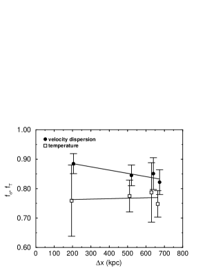
Figure 3: Normalizations for the M-T and M-$\sigma$ virial relations (as determined by numerical simulation) as a function of resolution, measured by cell size in kpc at $z=0$. The $f_{\sigma}$ points have been slightly offset in $\Delta x$ for clarity. Lines are the best-fit linear relation.

In Table 2.3.1, we also list the normalizations determined by other authors, using different numerical techniques. Evrard ([Evrard 1991], E91) performed 22 simulations of isolated clusters in an Einstein-de Sitter universe with a cold dark matter spectrum and obtained a somewhat larger normalization. The six ($\Omega=1$) clusters of NFW, using a TREESPH code, also had a slightly larger normalization. They used a marginally different virial overdensity, however when fitting their results to equation (4), we adopt their value of $\Delta_{c}=200$. The effect of increasing this parameter is to sample a slightly smaller volume, however since the velocity-dispersion profile is nearly flat in this range (c.f. section 4), the effect is very small. The P³M simulations of Crone and Geller (1995, CG95)cro95 resulted in a mean $f_{\sigma}=0.91$ (after converting from their notation) for well resolved clusters, with $\Delta_{c}=300$. This also found that the smallest clusters deviated slightly from the virial power-law, ascribing the effect, as we do, to insufficient numerical resolution. Their scatter appears similar to that found here. Finally, the P³M simulations of Cole & Lacey (1996, CL96) produced similar results. They did not fit the virial relation, but their Figure 3 indicates both that the virial relation is a reasonable fit and that there is not substantial variation from a power law over the range of masses examined. Jing & Fang (1994)jin94 argued for $f_{\sigma}=0.8$–0.9, but this was based on combined N-body and Press-Schechter comparisons, rather than directly from the $M-\sigma$ relation. Finally, a number of other authors have studied this issue but often in ways which make it difficult to compare directly to the virial formalism. For example, Walter & Klypin (1996) used a fixed cluster radius rather than one based on the mean overdensity.

In section 2.2, we mentioned that high-resolution N-body simulations indicate that the dark matter density profile does not follow the isothermal $r^{-2}$ profile but is instead given by equation (12), which has two parameters. If one ($\delta_{0}$) is set by the requirement that the mean density inside the virial radius is $\Delta_{c}$, the other is strongly correlated with mass ([Navarro, Frenk & White 1996]), so the mean radial profile is completely specified by the mass (or, more accurately, the redshift of formation). The implied value of $f_{\sigma}$ (i.e. the correction as compared to the isothermal profile), can be computed using Jeans equation ($\rho^{-1}d[\rho\sigma(r)^{2}]/dr=-d\phi/dr$; we assume the velocity dispersion is isotropic for simplicity). It is the ratio of the mass weighted velocity dispersion (squared) to the isothermal virial value:

$$f_{\sigma}^{2} = \frac{\bar{\sigma}^{2}}{\sigma_{vir}^{2}}=\frac{2c}{\left(\ln\left(1+c\right)-\frac{c}{1+c}\right)^{2}}\int_{0}^{c}y^{2}dy$$ (17)

$$\int_{y}^{\infty}\frac{dx}{x^{3}\left(1+x\right)^{2}}\left[\frac{1}{1+x}-1+\ln\left(1+x\right)\right]$$

For the range of masses and cosmologies studied here, c varies from 5-10, and the resulting $f_{\sigma}$ = 0.92-0.97.

Thus we have strong evidence from a variety of sources that the virial relation describes clusters fairly well, although the normalization may need to be slightly modified, with a value around $f_{\sigma}\sim 0.9$-0.95 in good agreement with a wide variety of numerical methods. Unfortunately, there is likely to be a systematic bias between the velocity dispersion of the dark matter and that of the galaxies ([Carlberg, Couchman & Thomas 1990]; [Summers, Davis & Evrard 1995]) which we cannot address with these simulations, so we turn to the thermal temperature of the gas for a better observational diagnostic.

2.3.2 The $M$-$T$ relation

The temperature-mass relation for our models is shown in Figure 4. The temperature is a bolometric- luminosity weighted average across the cluster. In contrast to the $M$-$\sigma$ relation, even the most poorly resolved clusters follow the virial relation, with the exception of the open model, in which very low mass clusters have a higher temperature than predicted. This may be due to the earlier formation times for these clusters, as compared to the other models ([Navarro, Frenk & White 1996]).

Figure 4: The virial mass and emissivity-weighted temperature of clusters for the same models and redshifts as in Figure 2. Lines are the virial scaling relations from equation (9), with normalizations given in Table 2.3.1.

As before, the virial relations are fit with the 25 most massive clusters at $z=0$, and the results, as parameterized by $f_{T}$ are given in Table 2.3.1 and plotted against cell size in Figure 3. There is no discernible trend with resolution.

In the same Table, we also show the value of $f_{T}$ as determined by other simulations, all of which used smoothed particle hydrodynamics (SPH). The cluster simulations of Evrard (1991) produced a normalization very close to that obtained here, although he used a mass-weighted temperature. The six clusters of NFW again indicate a slightly higher value, although still within 10%. Recently, Evrard, Metzler & Navarro (1996, EMN96) examined simulations of 58 clusters (a sample which included the six of NFW) for a variety of models, including those with low $\Omega$. For $\Delta_{c}=250$, they find a mean value of $f_{T}=0.92$. This is 17% above our mean result. A careful examination of their Figure 4 indicates that there are slight systematic differences between the simulations, with clusters in flat universes implying somewhat lower values for $f_{T}$, and $\Omega=0.2$ (flat and open) models indicating higher normalizations. They also included a set of clusters which included substantial galactic winds, which appears to increase the virial normalization only very slightly. In it is interesting to note that the other physical contribution which we have not included here, cooling flows, would tend to decrease $f_{T}$, although the expected effect is quite small.

The range exhibited in Table 2.3.1 is surprisingly low, considering the range of models, resolutions, numerical techniques and researchers who have examined this robust relation. The size of the scatter is also quite low, around 10% (corresponding to a 15% scatter in mass). This implies that the temperature is an excellent virial mass indicator, even better than using $\beta$-model estimates ([Evrard, Metzler & Navarro 1996]).

2.3.3 The $T$-$\sigma$ relation

The relation between temperature and velocity dispersion is plotted in Figure 5, along with equation (7) for three values of $\beta$ (0.8,1,1.2). All simulations show curves which are steeper than predicted and there is a trend with mass, moving from low to high to values of $\beta$. This is probably a reflection of the fact that low mass clusters are more poorly resolved and so have a lower $\sigma$ than predicted (see also the $M$-$\sigma$ relation). The best resolved clusters, in fact, have values above one. This follows from the $M$-$T$ and $M$-$\sigma$ relations, since $\beta=f_{\sigma}^{2}/f_{T}\approx 1.06$. This value is close to the mean of NFW (1.07) but somewhat lower than the 1.18 found by Evrard (1991). Our result should most likely be viewed as a lower limit, since Figure 3 indicates that the $\sigma$ values have not yet converged. The most likely explanation for $\beta>1$ is incomplete thermalization in the gas, although since the two value are computed with different weights, this is not completely straightforward.

Figure 5: The velocity-dispersion and emissivity-weighted temperature of clusters identified for the same models and redshifts as in Figure 2, along with the scaling relation from equation (7).

Observationally, the quantity $\beta$ has been the subject of some investigation, with values being generally compatible with one ([Girardi et al. 1996]; [Lubin & Bahcall 1993]), although this is for the galaxy velocity dispersion rather than the collisionless component. See also Lubin et al. (1996)lor96.

2.3.4 The $M$-$L_{bol}$ relation

Figure 6 shows the mass-bolometric luminosity relation for our three models. Shown are both the virial predictions from equation (10) as thin lines, and the resolution-adjusted equation (15), as thick curves. The latter relation fits the simulated clusters quite well. As we demonstrated in section 2.2, a cluster’s luminosity is diminished by a factor which depends on its mass (and the resolution of the simulation). Another way to say this is that the core radius of the cluster is set by the the cell size, rather than scaling with cluster mass and density. Although the slopes differ, the variation in redshift for the two relations is very similar. Also, we should note that the curves are not fit (as for the $M$-$T$ and $M$-$\sigma$ relations), but all have the same, somewhat arbitrary, normalization given in section 2.1.

Figure 6: The mass and bolometric luminosity of clusters identified for the same models and redshifts as in Figure 2. Thin curves are the virial scaling relation from equation (10), while thick lines are from the resolution-adjusted version, equation (15).

2.3.5 The $L_{bol}$-$T$ relation

The final comparison is the bolometric luminosity-temperature relation (Figure 7). Although it is not independent of the previous four, it is the one with the best observational constraints. The observations indicate a slope of $L\sim T^{2.7\hbox{-}3.5}$ ([Edge & Stewart 1991a],b; [David et al. 1993]). Although the slope of the simulated clusters is closer to the observations than that predicted by the equation (11), we argue that this is an artifact of our fixed numerical resolution. This result applies to Eulerian simulations in general. Bryan et al. (1994b)chdm_xray found a slope in agreement with observations for the 2–10 keV luminosity-temperature (as opposed to the bolometric result presented here). As we see here, this was partly due to resolution effects (but also resulted from the finite band-pass which strongly curtails the luminosity for clusters under a few keV). Thus, the basic discrepancy between the observed and predicted bolometric $L-T$ relation remains unresolved. Additional physics, such as galactic feedback, seems to be required (see also Evrard & Henry (1991)eh91 and NFW).

Figure 7: The temperature and bolometric luminosity of clusters identified for the same models, redshifts and virial relations as in Figure 6. The dot-dashed line indicates the observed relation $L\sim T^{3}$ at $z=0$.

2.3.6 Scatter in the virial relations

The scatter of clusters around the virial relations can be important because it provides a limit on how accurately masses can be determined, even in the absence of observational uncertainties. This is a factor in computing distribution functions of observable quantities, such as temperature or luminosity, since a given mass is associated with a range of temperatures. More concretely, given a mass distribution $dn/dM$, the resulting temperature function $dn/dT$ (computed by multiplying by the virial relation $dM/dT$) must be convolved with the scatter.

Figure 8: Cumulative distributions of $f_{\sigma}$ (top) and $f_{T}$ (bottom) for the 25 most massive clusters in our three primary simulations. The solid lines are Gaussian distributions fitted to the combined sample.

In Figure 8, we show cumulative distribution functions for our three canonical simulations. Although the $f_{\sigma}$ relation is somewhat tighter than $f_{T}$, their accuracy in predicting the cluster mass is nearly identical (since $M\sim\sigma^{3}\sim T^{3/2}$). As we noted previously, the mean of the velocity dispersion distribution appears to shift slightly with resolution, but the temperature does not. The shape of the distributions are well described by a Gaussian (as verified by a Kolmogorov-Smirnov test).

In order to compare the size of the fluctuations to those observed in real clusters, we must use the $L$-$T$ relation. Although the slope of our predicted relation disagrees with that observed, we can compare the scatter around the two curves. Since real cluster temperatures also have observational uncertainties, we add the intrinsic scatter and observed uncertainty in quadrature. The simulated clusters have a scatter of $11.4^{+2.3}_{-1.4}$%. The flux-limited sample of Henry & Arnaud (1991) gives $19.6^{+4.4}_{-2.7}$% (similar to, but slightly higher than, the 16.4% found by Pen, 1996, for the same sample), while the larger sample of David et al. (1993) requires a smaller intrinsic scatter: $15.3^{+1.9}_{-1.5}$%. These values are determined by fitting the $L$-$T$ relation and adjusting $\sigma_{T}=fT$ until the resulting $\chi^{2}$ indicates a good fit; uncertainties are one sigma. Although the scatter in the simulated clusters appears to be lower than that observed, there are two factors which would lead us to overestimate the observed value. The first, which is unlikely to be important, is ignoring the small observational uncertainties in the luminosity. More seriously, we have implicitly assumed that the temperature uncertainties are normally distributed. Since most realistic distributions have tail probabilities that are larger than Gaussian, this causes us to overvalue outliers, forcing the required intrinsic scatter to rise. In any case, the difference is not large, and so we tentatively conclude that the simulations reproduce the observed scatter.

3 Distribution Functions

The scaling relations discussed in the previous section can be combined with a prescription for computing the mass distribution function of virialized objects to make predictions of more easily observed distribution functions. Although there are many prescriptions for obtaining the number of collapsed objects given a power spectrum of linear initial perturbations (e.g. [Lacey & Cole 1993]; [Kitayama & Suto 1996]; [Bond & Myers 1996a]), we adopt the Press-Schechter (PS) formalism ([Press & Schecter 1974]) because it is fairly accurate, relatively simple, and widely used.

The comoving number of virialized objects of mass $M$ in mass interval $dM$ is given by,

$$\frac{dn}{dM}=\left(\frac{2}{\pi}\right)^{1/2}\frac{\bar{\rho}}{M}\frac{\nu_{c}}{\sigma(M)}\frac{d\bar{\sigma}}{dM}\>e^{-\nu_{c}^{2}/2}.$$ (18)

where $\bar{\rho}$ is the mean density and $\nu_{c}=\delta_{c}/\sigma(M)$. The linear rms density fluctuations of the power spectrum is given by

$$\sigma^{2}(M)=\int W_{T}^{2}(kR)P(k)d^{3}k$$ (19)

on the scale $M=4\pi R^{3}\bar{\rho}/3$ with a top-hat smoothing filter $W_{T}(x)=3(\sin(x)/x-\cos(x))/x^{2}$ [note the difference between the velocity dispersion $\sigma$ and the rms density fluctuation $\sigma(M)$]. The numerical value of $\delta_{c}$ has been the topic of some debate. The spherical collapse model gives $\delta_{c}$ as a slowing varying function of cosmology which is well fit by: $\delta_{c}=1.686\Omega(z)^{c}$, where $c=0.055$ (0.018) for flat (zero cosmological constant) models. However, given the shortcomings of the theory’s theoretical underpinnings ([Bond et al. 1991]), it is probably a better approach to take $\delta_{c}$ as a free parameter and fit for it.

In Figure 9 we show the result of comparing halos from the simulation (identified with the spherical overdensity scheme described earlier) with predictions from equation (18) for the CDM270, CHDM512 and OCDM256 models at a few different redshifts. The agreement is generally good, although there are systematically fewer low mass clusters in the simulation than predicted. This is due in part to the fact that those clusters are poorly resolved, but also seems to be a general shortcoming of the PS method ([Bond & Myers 1996b]). All the simulations produced fewer high-mass clusters with increasing redshift, although the evolution is strongest in the model with massive neutrinos and weakest in the open cosmology. The number of massive clusters at higher redshifts (particularly around $z=1$) for the OCDM256 model is underpredicted. If this result is correct, then it makes the difference between open and flat models even larger than previously predicted by PS methods, however two comments are in order. First, this simulation has the smallest number of well-resolved clusters (CHDM512 has better resolution, while CDM270 has more and larger clusters). Second, the significance is small since the number of clusters involved is very small. Indeed, we should point out that these simulations are not the best to test the Press-Schecter methodology since purely N-body simulations can afford better resolution, and can use a larger box to produce more high mass clusters. Still, we press on to illustrate what we believe to be a more objective and informative way to constrain the parameter $\delta_{c}$.

Figure 9: The mass distributions function for the same models and redshifts as in Figure 2. Lines are Press-Schechter predictions with $\delta_{c}$ given by the spherical collapse model (see text).

We can be more quantitative about the fits by varying this parameter (fixed in Figure 9 by the spherical collapse prediction). Since the PS formalism is often used to constrain theories of structure formation, knowledge of the uncertainty in its predictions is important. We construct a likelihood estimator by considering the distribution of clusters above a mass cutoff $M_{\star}$ for each simulation. If we divide the range of masses into intervals $\Delta M$ that are sufficiently small so that the predicted number of objects in each range, $n(M)=\Delta Mdn/dM\ll 1$, then the probability of finding either 0 or 1 objects in this range is given by the Poisson distribution: $P(0)=\exp[-n(M)]$ or $P(1)=n(M)\exp[-n(M)]$. The relative likelihood of finding a particular set of clusters is the product of the probabilities for all the mass intervals, split into those with clusters and those without: $P(\delta_{c})=\prod P(1)\prod P(0)$. For $\Delta M\ll 1$, this can be written as:

$$P(\delta_{c})=\left[\prod_{i}\frac{dn(M_{i})}{dM}\Delta M\right]\exp\left[-\int_{M_{\star}}^{\infty}\frac{dn(M)}{dM}dM\right].$$ (20)

The product is over all the cluster masses $M_{i}$ above the cutoff $M_{\star}$; the distribution is normalized, so that $\int P(\delta_{c})d\delta_{c}=1$. To imitate the simulation as closely as possible, we have set the power spectrum to zero for scales larger than the fundamental wavelength of the box. This has only a slight effect, shifting $\delta_{c}$ by about 1%.

Figure 10 shows the resulting likelihood distributions for our three models. Since we are primarily interested in the higher mass clusters, we choose a mass cutoff ($M_{\star}$) of twice the non-linear mass (this is about $1\times 10^{14}M_{\odot}$ for the OCDM256 and CHDM512 cases and $6\times 10^{14}M_{\odot}$ for CDM270). The curves are reasonably well fit by Gaussians with means and one sigma uncertainties given by $1.84\pm 0.12,1.75\pm 0.12$ and $1.72\pm 0.09$ for CDM270, CHDM512 and OCDM256 respectively. These are all compatible with the spherical collapse prediction.

Figure 10: The likelihood distributions for $\delta_{c}$, as determined by our three models at $z=0$.

These values are in the range advocated by other authors ([Efstathiou et al. 1988]; [Narayan & White 1988]; [Carlberg & Couchman 1989]; [Bond et al. 1991]), although some caution is in order since we are comparing results with different methods for identifying clusters and their masses. For more recent work which adopts the same methodology as employed here, the agreement is remarkable. Lacey & Cole (1996)lac96 used scale-free simulations with a variety of cluster analysis techniques. For the spherical overdensity method with a top-hot filter, they find a best fit of $\delta_{c}=1.96$, however, this is over a considerable range in mass. For their rarest peaks (corresponding to the clusters discussed here), it appears that a normalization somewhat lower, but just above 1.68, is appropriate. Eke, Cole & Frenk (1996)eke96 found that a value around 1.75 gave good fits to very large ($350^{3}h^{-1}$Mpc³) simulations for a variety of cosmologies. Borgani et al. (1997)bor97 argue for $\delta_{c}$ near 1.68 (for a top-hat filter) based on a series of simulations including a cosmological constant term.

Finally, we note that a cluster identification based on mean overdensity does not necessarily produce a one-to-one correlation with bound halos. As we discuss in the section on temperature, this should not strongly affect our results, however it is important if one is interested in the details of bound halos. For a more complete discussion of the mass function of halos in the CDM model see Gelb & Bertschinger (1994)gel94.

The high-end of the mass function is exponentially sensitive to the amplitude of the power spectrum, so it is worthwhile examining the non-linear mass ($M_{nl}$), which controls the position of this cutoff. It is defined as the mass within a spherical volume for which the rms overdensity from equation (19) is equal to $\delta_{c}$. Figure 11 shows the evolution of this quantity, using both the linear power spectrum and the fully non-linear (N-body) spectrum (for a more complete discussion in terms of the CDM model, see [Jain & Bertschinger 1994]). This figures shows both the increased normalization of the CDM270 model, and the slower evolution of the OCDM256 mass function. Scale-free spectra with $P(k)\propto k^{n}$ result in $M_{nl}\propto(1+z)^{-6/(n+3)}$. The ordinate is $\log(1+z)$ so the these models would show up as straight lines on the plot. The linear results for CDM are closer to the non-linear than for the other models because of the shallower spectral profile (smaller logarithmic slope). In other words, the CHDM slope is close enough to $P(k)\sim k^{-3}$ that the extremely rapid evolution of $M_{nl}$ requires more accuracy to obtain a good estimate of the non-linear mass.

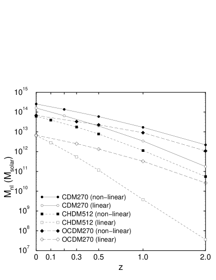
Figure 11: The evolution of the non-linear mass (see text for definition) for our three primary models, computed both through the linear and non-linear (N-body) power spectra.

Although useful, the mass distribution is difficult to obtain from observations because of uncertainties in obtaining the total mass out to the virial radius. Somewhat easier is the temperature distribution. In Figure 12, we plot this function for the canonical models as well as analytic predictions using Press-Schechter and the mass-temperature relation: equations (18) and (9). From the results of section 2, we adopt the mass-temperature normalization $f_{T}=0.77$, producing reasonable agreement between the simulations and analytic results. Again, there is are strong difference between the evolutionary properties. When medium to high redshift temperature samples become available, they will provide strong constraints.

We stress at this point that the temperature (and velocity dispersion) distribution functions are much more robust against variations in cluster identification shemes than the mass function. This is true because the mass is a rising function of radius (since $\rho\sim r^{-2}$), while, to first order, the temperature is constant. How can $N(>T)$ can be relatively independent of the cluster identification method, while $N(>M)$ — from which it is derived — is not? In fact, this is only true if the $N(>M)$ and the $T$-$M$ relation are calibrated consistently. In other words, if we change the way we find the cluster mass (within reason), the $T$-$M$ relation and the mass function will both change such that the resulting $N(>T)$ is unchanged. This feature of the temperature distribution is particularly important when it comes time to compare with observations, which are rarely determined to the virial radius.

Figure 12: The temperature distribution functions for the same models and redshifts as in Figure 2. Lines are predictions from the extended PS model with $\delta_{c}$ given by the spherical collapse model and $f_{T}=0.77$.

Since luminosities are more easily obtained observationally, we use equation (10) to determine the bolometric luminosity distribution with Bremsstrahlung radiation and zero metallicity (this constraint will be relaxed in the next section). These are shown as thin lines in Figure 13. While the simulated clusters do not match these results, including the effects of finite resolution with equation (10) does produce agreement, at least for the relative bright clusters. The ‘fully’ resolved Press-Schechter predictions show that, for the brightest clusters, there is positive evolution with redshift in the OCDM model but negative evolution for CHDM. However, the exact behaviour depends on the adopted $L$-$T$ relation. Since the fixed resolution produces an $L-T$ relation closer to that observed (albeit for numerical reasons), it may be the better predictor of evolution. In that case, the OCDM model is nearly constant over redshift, while the CHDM evolution is strong negative.

Perhaps more importantly, the difference between the thin and bold lines indicates the kind of error engendered by our limited spatial resolution. Roughly speaking, there are two effects. The first is the obvious reduction in the luminosity of all clusters, shifting the curves to the left. The other is to add an additional component of negative redshift evolution, exaggerating the negative evolution at high luminosities and decreasing the positive evolution at the low end, causing the curves to tilt slightly. This second effect is relatively small, about the size of Poisson fluctuations due to the limited number of clusters.

Figure 13: The bolometric luminosity distribution functions for the same models and redshifts as in Figure 2. The Press-Schechter results for two mass-luminosity relations are also shown: thin lines use equation (10) while bold lines include the effects of limited resolution: equation (15).

3.1 Metallicity Effects

In this section we address more realistic X-ray emissivity effects: limited band-passes and line emission from multiply ionized heavy elements in the plasma: metallicity. As we will show, for moderate and high temperature clusters, the ratio of line to continuum emission is actually quite small, only a few percent, making the accurate determination of a cluster’s metallicity difficult. On the positive side, this make our results largely insensitive to the assumed metallicity. Nevertheless, the high resolution spectroscopy performed by the ASCA satellite, as well as work done with ROSAT and other missions, seems to indicate that a value of $Z/Z_{\odot}=0.3$ in solar units is reasonable for many clusters ([Kowalski et al. 1993]; [Markevitch et al. 1994]).

We use a Raymond-Smith code (1977, 1992 version)ray77 to compute emissivities which are shown in the top panel of Figure 14 for a variety of metallicities and band-passes as a function of temperature assuming a number density of electrons of $10^{-3}$ cm^-3. The effect of line emission from metals is small for $T>2$ keV. This means that previous results ([Bryan et al. 1994a],b) computed with the assumption of zero-metallicity will not be substantially affected in the region where observational results are most plentiful. Nevertheless, this will prove important for small clusters and groups of galaxies so we extend our previous analytic results to include this effect (although, of course, our simulations do not include many other effects that may prove important for small clusters such as stellar feedback and radiative cooling).

To do this, we fit simple expressions to the full result by ignoring the temperature variation of the gaunt factor and approximating the effect of metallicity as a power law with a cutoff. The resulting formula is given in relation to the bolometric luminosity ($L_{metal}=\epsilon(Z,T,\nu_{1},\nu_{2})L_{bol}$, where $\nu_{1}$ and $\nu_{2}$ specify the band-pass) by:

$$\epsilon(Z,T,\nu_{1},\nu_{2}) = \left[\exp(\frac{-h\nu_{1}}{kT})-\exp(\frac{-h\nu_{2}}{kT})\right]\times$$ (23)

$$\left\{\begin{array}[]{ll}(kT/2\hbox{ keV})^{-\gamma\sqrt{\frac{Z}{0.3Z_{\odot}}}}&kT<2\hbox{ keV}\\ 1&kT>2\hbox{ keV}\end{array}\right.$$

The effect of metallicity depends on the bandpass used and cannot be simply modelled, so we parameterize it through $\gamma$ and tabulate values appropriate for a few common choices: $\gamma=0.6$ for 0.1–2.4 keV; 0.9 for 0.5–2.4 keV; 0.0 for 2–10 keV; and 0.7 for bolometric luminosities (we use $g_{ff}=1.3$, and 24% He by mass). This fit is accurate to only about a factor of two, but will be sufficient for our purposes; a few examples are shown in the bottom panel of Figure 14.

Figure 14: The X-ray emissivity as a function of temperature for two different metallicities and three different band-passes from a Raymond-Smith code (top panel). The relative X-ray emissivity (normalized to the bolometric emissivity at that temperature for a metal-free plasma) as thin lines (bottom panel). Also shown in thick lines are the approximate fits from equation (23).

With this extension we can now compute more observationally oriented luminosity functions and compare them to the luminosity function computed directly from the simulation. The numerical cluster luminosities are computed on a cell-by-cell basis so they include the spatial variation of temperatures (see section 4), which the analytic models are missing. They also use emissivities calculated from the full Raymond-Smith code. Figure 15 shows the luminosity function in the 0.1-2.4 keV bandpass for a representative case (CDM270 at $z=0$). The PS model overpredicts the number of low-luminosity clusters, just as it does for low mass clusters, however the general effect of metallicity is included correctly. This also demonstrates that the effects of metallicity are negligible above about $10^{44}$ erg/s and relatively slight above $10^{43}$ erg/s.

Figure 15: The 0.1-2.4 keV luminosity distribution function with (dashed) and without (solid) metallicity for the CDM270 model. The extended Press-Schechter results are also shown, with the usual meaning for thin and thick lines.

4 Cluster structure

In deriving some of the analytic results we assumed a spherically symmetric isothermal profile for both the gas and dark matter. In this section we examine the simulated clusters in order to determine the accuracy of these assumptions. A more complete analysis will be presented in Bryan & Norman (1997b)bry97b.

In Figure 16 we show profiles of temperature and the one-dimensional velocity dispersion for the five most massive clusters in our two canonical models. These are normalized by their appropriate virial values (with $f_{T}=f_{\sigma}=1$). To compute the profile, we redetermine the cluster centers by adopting the center of the cell with the highest gas density within $r_{vir}/2$ of the original center found through the iterated spherical overdensity method. This procedure does a good job of finding the core of the largest mass clump. The innermost point plotted is two cell widths from the cluster center. This is approximately our resolution limit.

Figure 16: Temperature (top panel) and dark matter one-dimensional velocity dispersion (bottom panel) profiles for the CDM270 and the CHDM512 models at $z=0$, normalized by their respective virial values.

The spherically-averaged temperature profiles are compatible between models and show a very slowly falling profile to about $0.7r_{vir}$, a somewhat steeper slope ($r^{-0.5}$) to about two times the virial radius and then a very sharp fall off beyond that. The velocity profiles are close to flat, although they appear to show a slight dip at and just before the virial radius. They are also slightly below their respective $\sigma_{vir}$ values (implying $f_{\sigma}<1$). However, this tendency may be declining as we resolve further towards the center. The hot component (we plot only the cold particles in Figure 16) follows almost exactly the same profile at large r, but is systematically higher at low radii. The temperature profile shows much greater variation and is less compatible with an isothermal model, even after spherical averaging. The temperature and $\sigma$ profiles are in agreement with the factors $f_{T}\sim 0.8$ and $f_{\sigma}\sim 0.85$-0.9 derived earlier.

5 Conclusion

In this paper, we have shown that X-ray clusters produced in Eulerian simulations agree well with the scaling relations involving mass, temperature and the collisionless velocity dispersion. The luminosity behaviour is more affected by resolution but can be simply and accurately modelled. The predicted bolometric $L$-$T$ relation does not match that observed. We argue that this is mostly the fault of the luminosity prediction since it is very sensitive to the structure of the clusters, while the temperature is not. Indeed, the mass-temperature relation appears to be remarkably robust and, as we have demonstrated, depends very little on the input physics, numerical method, resolution, or cosmology. Our result, combined with a review of the available literature, indicates that $f_{T}\approx 0.8$ in the notation of equation (9). We also demonstrated that the isothermal profile assumed in computing the normalization of the scaling relation between $M$ and $\sigma$ is a reasonable approximation for the dark matter (although there is evidence for $f_{\sigma}<1$).

We stress here the difference between $f_{T}$, $f_{\sigma}$ and $\beta$. The first two adjust the virial scaling relation normalizations as compared to the hydrostatic isothermal sphere assumption, while $\beta$ is the ratio of the collisionless ‘temperature’ to the gas temperature, equation (7). These three quantities are related through $\beta=f_{\sigma}^{2}/f_{T}$. Since prescriptions such as the Press-Schechter formalism predict the distribution of masses, the important normalizations are $f_{\sigma}$ and $f_{T}$ (of the $M$-$\sigma$ and $M$-$T$ relations, respectively), and not $\beta$, as is occasionally assumed (e.g. [Eke, Cole & Frenk 1996]).

Based on these findings and the Press-Schechter prescription for computing the differential number density of virialized halos, we computed the temperature distributions functions which are in good agreement with those derived from the numerical simulations (over their range of validity). In Figure 17, we show the temperature functions for our three models along with the 95% uncertainty in $\delta_{c}$. The observations ([Henry & Arnaud 1991]; [Eke, Cole & Frenk 1996]) are also shown, computed as $N(>T)=\sum_{T_{i}>T}1/V_{max,i}$ (where $V_{max,i}$ is the maximum volume for which the cluster with temperature $T_{i}$ and flux $f_{i}$ could have been observed). This shows that the CDM270 model predicts substantially too many clusters, while the CHDM512 and OCDM256 models are (very) marginally in agreement. The fits would be much improved if the power spectra were renormalized to $\sigma_{8}=0.55,0.63,0.85$ for CDM270, CHDM512 & OCDM256. To retain agreement with COBE, the CHDM model would require only a slight tilt. This result differs slightly from Ma (1996)ma96 due to the addition of a second neutrino. Otherwise, for the same $Q_{rms-PS}$ we would have to increase $\sigma_{8}$ by 10% ([Stompor, Gorski & Banday 1995]). The OCDM270 model could also be adjusted slightly to match both COBE and clusters, however, CDM would require a large tilt in the spectrum ($n\sim 0.8$).

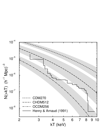
Figure 17: The PS temperature distribution functions for our three primary models at $z=0$ using the best fit $\delta_{c}$ for each model. Shaded regions are the two-sigma uncertainties in $\delta_{c}$. Observations from Henry & Arnaud (1991)hen91 are shown as a solid line.

Analytic luminosity functions computed with the effects of finite resolution (Figure 13) agree well with the simulations and allow us to gauge the impact of resolution as a function of luminosity and redshift. An extension which accounts for metallicity and limited bandpass, equation (23), can be used to compare directly against observational data. Just as we used the temperature distribution function, we could also use the luminosity to compare to observations, however, the observational luminosity-temperature relation does not agree with the scaling relations. Using the observed $L$-$T$ relation to compute $n(>L)$ from $n(>T)$ does not add any additional information, since if we match the temperature function we must also match the luminosity function. However, recent observations with the ASCA satellite have produced a sample of temperatures at moderate redshift ([Mushotzky & Scharf 1997]). The sample is not complete so we cannot use it to construct a temperature function, however it can be used to constrain evolution in the observed $L$-$T$ relation. Combined with the method for predicting $n(>T)$ described in this paper and the upcoming high redshift luminosity samples ([Romer et al. 1997]; [Scharf et al. 1997]), we will be able to place much tighter constraints on the models based on cluster evolution.

This work is done under the auspices of the Grand Challenge Cosmology Consortium and supported in part by NSF grants ASC-9318185 and NASA Long Term Astrophysics grant NAGW-3152.

References

- [Anninos & Norman 1994] Anninos, P., Norman, M.L., & Clarke, D.A. ApJ, 436, 11
- [Anninos & Norman 1996] Anninos, P. & Norman, M.L. 1996, ApJ, 459, 12
- [Bardeen et al. 1986] Bardeen, J.M., Bond, J.R., Kaiser, M., & Szalay, A.S. 1986, ApJ, 304, 15
- [Binney & Tremaine 1987] Binney, J. & Tremain, S. 1987, Galactic Dynamics (Princeton: Princeton University Press), p. 228
- [Bond et al. 1991] Bond, J.R., Kaiser, N., Cole, S., Efstathiou, G. 1991, ApJ, 379, 440
- [Bond & Myers 1996a] Bond, J.R. & Myers, S.T. 1996a, ApJS, 103, 1
- [Bond & Myers 1996b] Bond, J.R. & Myers, S.T. 1996b, ApJS, 103, 41
- [Borgani et al. 1997] Borgani, S., Moscardini, L., Plionis, M., Górski, K.M., Holtzman, J., Klypin, A., Primack, J.R., Smith, C.C., Stompor, R. 1997, New Astronomy, 1, 321
- [Bryan et al. 1994a] Bryan, G.L., Cen, R., Norman, M.L., Ostriker, J.P., Stone, J.M. 1994a, ApJ, 428, 405
- [Bryan et al. 1994b] Bryan, G.L., Klypin, A., Loken, C., Norman, M.L., Burns, J.O. 1994b, ApJ, 437, L5
- [Bryan et al. 1995] Bryan, G.L., Norman, M.L., Stone, J.M., Cen, R., Ostriker, J.P. 1995, Comput. Phys. Comm., 89, 149
- [Bryan & Norman 1997a] Bryan, G.L. & Norman, M.L. 1997a, to appear in Proc. 12th Kingston Meeting on Theoretical Astrophysics
- [Bryan & Norman 1997b] Bryan, G.L. & Norman, M.L. 1997b, in preparation
- [Burns et al. 1996] Burns, J.O., Ledlow, M.J., Loken, C., Klypin, A., Voges, W., Bryan, G.L., Norman, M.L., White, R.A. 1996, ApJ, in press
- [Carlberg & Couchman 1989] Carlberg, R.G. & Couchman, H.M.P. 1989, ApJ, 340, 47
- [Carlberg, Couchman & Thomas 1990] Carlberg, R.G., Couchman, H.M.P., Thomas, P.A. 1990, ApJ, 352, 29
- [Cen 1992] Cen, R. 1992, ApJS, 78, 341
- [Cole & Lacey 1996] Cole, S. & Lacey, C. 1996, preprint (astro-ph/9510147)
- [Couchman, Thomas & Pearce] Couchman, H.M.P., Thomas, P.A., Pearce, F.R. 1995, ApJ, 452, 797
- [Crone, Evrard & Richstone 1994] Crone, M.M., Evrard, A.E., Richstone, D.O. 1994, ApJ, 434, 402
- [Crone & Geller 1995] Crone, M.M., & Geller, M.J. 1995, ApJ, 110, 21
- [David et al. 1993] David, L.P., Slyz, A., Jones, C., Forman, W., & Vrtilek, S.D. 1993, ApJ, 412, 479
- [Ebeling et al. 1995] Ebeling, H., Allen, S.W., Crawford, C.S., Edge, A.C., Fabian, A.C., Böhringer, H., Voges, W., Huchra, J.P., to appear in Röntgenstrahlung from the Universe, Würzburg 1995.
- [Edge et al. 1990] Edge, A.C., Stewart, G.C., Fabian, A.C., Arnaud, K.A. 1990, MNRAS, 245, 559
- [Edge & Stewart 1991a] Edge, A.C. & Stewart, G.C. 1991a, MNRAS, 252, 414
- [Edge & Stewart 1991b] Edge, A.C. & Stewart, G.C. 1991b, MNRAS, 252, 428
- [Eke, Cole & Frenk 1996] Eke, V.R., Cole, S., & Frenk, C.S. 1996, MNRAS, submitted
- [Efstathiou et al. 1988] Efstathiou, G., Frenk, C.S., White, S.D.M., Davis, M. 1988, MNRAS, 235, 715.
- [Evrard 1991] Evrard, A.E. 1991, in Clusters of Galaxies, ed. M. Fitchett & W. Oegerle (Cambridge: Cambridge Univ. Press)
- [Evrard & Henry 1991] Evrard, A.E., Henry J.P. 1991, ApJ, 383, 95.
- [Evrard 1988] Evrard, A.E. 1988, MNRAS, 235, 911
- [Evrard, Metzler & Navarro 1996] Evrard, A.E., Metzler, C.A. & Navarro, J.F. 1996, ApJ, 469, 494
- [Gelb & Bertschinger 1994] Gelb, J.M., & Bertschinger, E. 1994, ApJ, 436, 467
- [Girardi et al. 1996] Girardi, M., Fadda, D., Mardirossian, F., Mezzetti, M., Biviano, A. 1996, ApJ, 457, 61
- [Henry & Arnaud 1991] Henry, J.P., & Arnaud, K.A. 1991, ApJ, 372, 410
- [Henry et al. 1992] Henry, J.P., Gioia, I.M, Maccacaro, T., Morris, S.L., Stocke, J.T., & Wolter, A. 1992, ApJ, 386, 408
- [Henry et al. 1995] Henry, J.P., Gioia, I.M., Huchra, J.P., Burg, R., Mclean, B., Böhringer, H., Bower, R.G., Briel, U.G., Voges, W., MacGillivray, H., Cruddace, R.G. 1995, ApJ, 449, 422
- [Hernquist & Katz 1989] Hernquist, L. & Katz, N. 1989, ApJS, 70, 419
- [Jain & Bertschinger 1994] Jain, B. & Berstchinger, E. 1994, ApJ, 431, 495
- [Jing & Fang 1994] Jing, Y.P. & Fang, L.Z. 1994, ApJ, 432, 438
- [Kaiser 1986] Kaiser, N. 1986,MNRAS, 222, 323
- [Kang et al. 1994a] Kang, H., Cen, R.Y., Ostriker, J.P., & Ryu, D. 1994a, ApJ, 428, 1
- [Katz, Weinberg & Hernquist 1996] Katz, N., Weinberg, D. , Hernquist, L. 1996, ApJS, 105, 19
- [Kitayama & Suto 1996] Kitiyama, T. & Suto, Y. 1996, MNRAS, in press
- [Klypin et al. 1994] Klypin, A., Borgani, S., Holtzman, J., Primack, J. 1994, ApJ, 444, 1
- [Kofman et al. 1995] Kofman, L., Klypin, A., Pogosyan, D., Henry, J.P. 1995, ApJ, 470, 102
- [Kowalski et al. 1993] Kowalski, M.P., Cruddace, R.G., Snyder, W.A., Fritz, G.G. 1993, ApJ, 412, 489
- [Lacey & Cole 1993] Lacey, C. & Cole, S. 1993, MNRAS, 262, 627
- [Lacey & Cole 1996] Lacey, C. & Cole, S. 1996, MNRAS, submitted
- [Lubin & Bahcall 1993] Lubin, L.M., Bahcall, N.A. 1993, ApJ, 415, L17
- [Lubin et al. 1996] Lubin, L.M., Cen, R., Bahcall, N.A., & Ostriker, J.P. 1996, ApJ, 460, 10
- [Ma & Bertschinger 1994] Ma, C.-P. & Bertschinger, E. 1994, ApJL, 434, 5
- [Ma 1996] Ma, C.-P. 1996, preprint (astro-ph/9605198)
- [Markevitch et al. 1994] Markevitch, M., Yamashita, K., Furuzawa, A., Tawara, Y. 1994, ApJ, 436, L71
- [Metzler & Evrard 1994] Metzler, C. & Evrard, A. 1994, ApJ, 437, 564
- [Mould et al. 1995] Mould, J., Huchra, J. P., Bresolin, F., Ferrarese, L., Ford, H. C., Freedman, W. L., Graham, J., Harding, P., Hill, R. Hoessel, J. G., Hughes, S. M., Illingworth, G. D., Kelson, D., Kennicutt, R. C., Jr., Madore, B. F., Phelps, R., Stetson, P. B., Turner, A. 1995, ApJ, 449, 413
- [Mushotzky & Scharf 1997] Mushotzky, R.F. & Scharf, C.A. 1997, preprint (astro-ph/9703039).
- [Narayan & White 1988] Narayan, R. & White, S.D.M. 1988, MNRAS, 231, 97
- [Navarro & White 1993] Navarro, J.F., & White, S.D.M. 1993, MNRAS, 265, 271
- [Navarro, Frenk & White 1995] Navarro, J.F., Frenk, C.S., White, S.D.M. 1995, MNRAS, 275, 720
- [Navarro, Frenk & White 1996] Navarro, J.F., Frenk, C.S., White, S.D.M. 1994, ApJ, 462, 563
- [Peebles 1980] Peebles, P.J.E. 1980, The Large-Scale structure of the Universe (Princeton: Princeton University Press)
- [Pen 1997] Pen, U.-L. 1997, preprint (astro-ph/9610147)
- [Press & Schecter 1974] Press, W.H., & Schecter, P. 1974, ApJ, 187, 425
- [Raymond & Smith 1977] Raymond, J.C. & Smith, B.W. 1997, ApJS, 35, 419
- [Romer et al. 1997] Romer, A.K., Nichol, R.C., Collins, C.A., Burke, D.J., Holden, B.H., Metevier, A., Ulmer, P, Pildis, R. 1997, to appear to Proceedings of the 18th Texas Symposium on Relativistic Astrophysics (astro-ph/9701233).
- [Ruiz-Lapuente 1996] Ruiz-Lapuente, P. 1996, ApJ, 465, 83L
- [Ryu et al. 1993] Ryu, D., Ostriker, J.P., Kang, H., & Cen, R. 1993, ApJ, 414, 1
- [Scharf et al. 1997] Scharf, C.A., Jones, L.R., Perlman, E., Ebeling, H., Wegner, G., Malkan, M., Horner, D. 1997, to appear to Proceedings of the 18th Texas Symposium on Relativistic Astrophysics (astro-ph/9702009).
- [Shapiro et al. 1996] Shapiro, P.R., Martel, H., Villumsen, J.V., Owen, J.M. 1996, ApJS, 103, 269
- [Spitzer 1978] Spitzer, L. Jr. 1978, Physical Processes in the Interstellar Medium (New York: Wiley)
- [Stompor, Gorski & Banday 1995] Stompor, R., Gorski, K.M., Banday, A.J. 1995, MNRAS, 277, 1225
- [Summers, Davis & Evrard 1995] Summers, F.J., Davis, M., & Evrard, A.E. 1995, ApJ, 454, 1
- [Walter & Klypin 1996] Walter, C. & Klypin, A. 1996, ApJ, 462, 13
- [White 1995] White, D.A. & Fabian, A.C. 1995, MNRAS, 273, 72
- [White et al. 1993] White, S.D.M., Navarro, J.F., Evrard, A.E., & Frenk, C.S. 1993, Nature, 366, 429