The Quasi-Stationary Structure of Radiating Shock Waves.
I. The One-Temperature Fluid
Abstract
We calculate the quasi-stationary structure of a radiating shock wave propagating through a spherically symmetric shell of cold gas by solving the time-dependent equations of radiation hydrodynamics on an adaptive grid. We show that this code successfully resolves the shock wave in both the subcritical and supercritical cases and, for the first time, we have reproduced all the expected features – including the optically thin temperature spike at a supercritical shock front – without invoking analytic jump conditions at the discontinuity. We solve the full moment equations for the radiation flux and energy density, but the shock wave structure can also be reproduced if the radiation flux is assumed to be proportional to the gradient of the energy density (the diffusion approximation), as long as the radiation energy density is determined by the appropriate radiative transfer moment equation.
We find that Zel’dovich and Raizer’s analytic solution for the shock wave structure accurately describes a subcritical shock but it underestimates the gas temperature, pressure, and the radiation flux in the gas ahead of a supercritical shock. We argue that this discrepancy is a consequence of neglecting terms which are second order in the minimum shock compression ratio [, where is the adiabatic index] and the inaccurate treatment of radiative transfer near the discontinuity. In addition, we verify that the maximum temperature of the gas immediately behind the shock is given by , where is the gas temperature far behind the shock.
Keywords: radiating shock waves – numerical methods
Correspondence to: M. W. Sincell
1 Introduction
The structure and dynamics of radiative shock waves in astrophysical fluids are difficult to model because processes in the shock front occur on length scales that are many orders of magnitude smaller than the typical length scales for other gradients (e.g., the velocity field in an accretion flow) in the fluid variables. There are two standard methods for computing the structure of shocked fluids. The first is to treat the shock as a discontinuity and invoke conservation laws to relate physical quantities on either side of the shock. Analytic models of shock waves have been constructed using this approach (e.g., Zel’dovich and Raizer 1967, Heaslet and Baldwin 1963) but these solutions require many simplifying assumptions which limit the applicability of the results. Time-dependent analytic solutions can be constructed for only the simplest of model problems (Zel’dovich and Raizer 1967). The second method is to introduce an expression for the viscosity in the shock. This is most common in numerical solutions, where an artificial viscosity is introduced to spread the shock over a few grid points. Numerical solutions can be hampered by the large gradients encountered at the shock front, which lead to unmanageably small time steps and numerical instabilities. To overcome these difficulties, the magnitude of the artificial viscosity is usually chosen to be many orders of magnitude larger than the physical viscosity.
Formulating the numerical problem on an adaptive grid can dramatically increase the effective resolution of the grid and reduce the spurious effects of artificial viscosity. Dorfi and Drury (1987) solved the one-dimensional hydrodynamic equations on an adaptive grid. They adopted a simple grid equation which distributes grid points uniformly along the arc length of a graph of the solution variables and solved two standard problems: the shock tube and a spherical blast wave. In both cases, the adaptive grid concentrated many grid points at discontinuities in the flow. Although artificial viscosity is still needed to spread the discontinuity over a few grid points, the physical separation of each point is negligible and the shock front appears infinitely steep. Gehmeyr and Mihalas (1994) demonstrated that this same equation can be used to resolve discontinuities in radiating flows and, in particular, they performed a preliminary numerical study of radiating shock waves. We extend the work of Gehmeyr and Mihalas (1994) in this paper.
An analytic description of the structure of a simple radiating shock front is presented in Zel’dovich and Raizer 1967. The gas upstream of the shock is assumed to be cold (, see Fig. 1) and at rest. A piston (speed ) drives a shock wave into the cold gas and the wave propagates into the unshocked material at a speed . The structure of the shock front is steady when viewed in a reference frame moving with the front and, in this frame, the upstream gas flows into the shock at the shock speed . The temperature of the shocked gas rises as the kinetic energy of the cold gas flowing into the shock is converted into internal energy of the material flowing out of the shock. The shocked gas moves away from the discontinuity at a velocity , which equals the speed of a piston driving the gas. The gas pressure and density also increase discontinuously at the shock front. The material upstream is preheated by radiation from the downstream shocked material; this raises the temperature of the inflowing material ahead of the shock and cools the gas behind the shock.
Zel’dovich and Raizer (1967) found that radiating shocks can be divided into two categories, subcritical and supercritical, which have qualitatively different structures. The shock wave is subcritical if the gas temperature just ahead of the shock front () is smaller than the final post shock temperature (). In this case, the absorption of radiation by the cold gas raises the preshock temperature to . The gas immediately behind the discontinuity is heated to by compression in the shock front and then cools radiatively until reaching the final temperature downstream from the shock. Radiation from the shocked gas is absorbed by inflowing cold gas and the gas temperature ahead of the shock declines exponentially with increasing optical depth, measured from the discontinuity. A cartoon of the subcritical shock structure is presented in Fig. 1a.
If the shock wave is strong enough, radiation from the shocked gas heats the material upstream from the shock until and the shock becomes supercritical. Viscous heating raises the temperature of the shocked gas from to just ahead of the discontinuity and the post-shock gas cools radiatively back to . The length scales for viscous heating and radiative cooling are much less than a radiation mean free path and the temperature spike () at the gas pressure discontinuity (indicated by a vertical dashed line in Fig. 1b) is optically thin. The upstream temperature can never exceed the downstream temperature because that would result in a discontinuity in the radiation flux and accumulation of radiation energy density, contradicting the steady state assumption (Zel’dovich 1957). The gas temperature ahead of the shock falls slowly because the radiation field remains in equilibrium with the gas. The gas temperature starts to drop exponentially several radiation mean free paths upstream of the shock because the gas and radiation fall out of equilibrium. A cartoon of the supercritical shock structure is presented in Fig. 1b.
In this paper we present time-dependent calculations of the structure of radiating shock waves for a simple model problem, in which a supersonic piston drives a shock wave through a spherical shell of cold gas at a constant density. This test problem is simple enough that we can compare directly to the analytic solutions of Zel’dovich and Raizer (1967), both as a test of the code and to determine the accuracy of the analytic solution. We describe the TITAN code in §2.1 and define the test problem in §2 We discuss our results in §3 and conclude in §4
2 Formulation of the Problem
2.1 Equations and Methodology
We use the TITAN code (Gehmeyr and Mihalas 1994) to solve the time-dependent equations of radiation hydrodynamics on an adaptive grid. Gehmeyr and Mihalas (1994) provide a detailed description of TITAN so we will only summarize the key features of the code here. The equations of radiation hydrodynamics in the single fluid approximation are the continuity equation
| (1) |
the gas momentum equation
| (2) |
the radiation momentum equation
| (3) |
the total (gas plus radiation) energy equation
| (4) |
and the radiation energy equation
| (5) |
where is the Lagrangean time derivative operator. We assume a perfect monatomic gas equation of state with an adiabatic index of with a constant absorptive opacity (). The radiation pressure () and energy density () are related by a variable Eddington factor, . The Eddington factors are computed with a formal integration of the time-independent radiative transfer equation (e.g., Mihalas and Mihalas 1984) and updated during each time-step. The remaining variables in these equations represent the radius (), the gas density (), gas velocity (), gas pressure (), gas energy per unit mass (), gas temperature () and radiation flux (). The physical constants in these equations, and those that follow, are the speed of light (), the radiation constant (), the proton mass (), the Stephan-Boltzmann constant () and the Boltzmann constant ().
We incorporate a tensor artificial viscosity (Tscharnuter and Winkler 1979, Gehmeyr and Mihalas 1994)
| (6) |
where
| (7) |
and is a constant of order unity.
The radiation hydrodynamics equation set (eqs. 1, 2, 3, 4 and 5) is supplemented with the adaptive grid equation (Gehmeyr and Mihalas 1994, Dorfi and Drury 1987). This equation distributes grid points so that discontinuities in the flow are resolved. The simplest examples of grids are the Eulerian grid, where the length scale is uniformly resolved, and the Lagrangean grid, where the mass of the gas is uniformly resolved.
The differential equations are written in finite volume form using the adaptive mesh transport theorem (Winkler, Norman and Mihalas 1984) and then expressed as algebraic finite difference equations on a staggered grid (Gehmeyr and Mihalas 1994). The difference equations are linearized around the current solution and the solution at the next time step is calculated with a fully-implicit Newton-Raphson iteration scheme.
2.2 The Model Problem
We consider a thin shell of gas extending from km to km, such as might be found around a neutron star. This problem is nearly plane parallel because . Initially, the gas is at rest with constant density ( g/cm3) and a shallow temperature profile
| (8) |
The sound speed in the gas is km/sec. The gas has a constant absorptive opacity cm-1. Initially, the gas and radiation are in equilibrium and that there is no net flux of radiation.
At time a piston at starts outward at a constant velocity, , and a shock forms ahead of the piston. The shock propagates outward at a velocity
| (9) |
where is the shock compression ratio and is the gas density behind the shock. Note that , where is the final compression ratio, because some additional compression can occur as the shocked gas cools from to . After a short time, , the shock reaches a quasi-stationary state in which the structure of the shock front is independent of time when viewed in a frame moving at a velocity , i.e., with the shock front.
In our simple model, the strength of the shock wave is determined by the piston speed. If all the kinetic energy of the gas ahead of the shock is converted into thermal energy of the gas behind the shock, then the post-shock gas temperature is
| (10) |
where is the piston speed in cm/sec, which is on the order of the sound speed in the gas.
2.3 Analytic Description of the Radiating Shock Front
In this section we review the analytic description of radiating shock waves. The reasons for this are twofold. First, the numerical and analytic calculations should be consistent in the regions of parameter space where the assumptions of the analytic description are valid. This provides a test of the numerical method. Second, the numerical model will be used to extend the analytic results into regions where the analytic approximations fail. For both applications, it is important to have a clear understanding of the assumptions of the analytic solution for the structure of the radiating shock front. Unless otherwise noted, the results in this section are found in Zel’dovich and Raizer (1967).
Zel’dovich and Raizer (1967) solve for the structure of a radiating shock wave in two steps. In the first step, they note that the equations of radiation hydrodynamics conserve mass, momentum and energy. These conservation laws translate into three first integrals, which can be written in terms of the gas compression ratio, :
| (11) |
where we have assumed and that both and vanish as . We adopt the convention that the radiation flux is positive outwards and set the mean molecular weight to , which is appropriate for a fully ionized hydrogen gas. We have also defined
| (12) |
the minimum post-shock compression ratio for a gas with an adiabatic index of . The conservation laws (eq. 2.3) must be satisfied by the flow outside of the shock front, where the viscosity is negligible.
The compressional work done on the inflowing gas and the change in the kinetic energy of that gas cancel to order . Expanding equations 2.3 to first order in , one finds
| (13) |
ahead of the shock. This relation expresses conservation of energy in the preheated gas.
The shocked gas cools from to over a radiation mean free path. This cooling takes place at nearly constant temperature, which implies that , where in the shocked gas. Expanding equations 2.3 to first order in , one finds the approximate energy conservation relation
| (14) |
In the analytic solution, equations 13 and 14 are the only link between the radiation transfer equations and the hydrodynamics.
The second step is the solution of the radiative transfer equation. In the case of a subcritical shock wave in a gas with a constant opacity, the radiation energy density is much larger than the equilibrium value and the radiative transfer equation is approximately independent of the gas temperature. This decouples the two steps. The gas and radiation field are in equilibrium near the discontinuity in a supercritical shock wave and the full set of radiation hydrodynamical equations must be solved simultaneously. Zel’dovich and Raizer (1967) invoke the approximate conservation law (eq. 13) to determine an analytic solution for the structure of a supercritical shock wave. In the following paragraphs we describe the analytic solution for both cases.
The shocked gas is optically thick and a flux emerges from the discontinuity. This flux cools the shocked gas and is then absorbed by the cold material ahead of the shock front. The post-shock gas temperature is fixed by the approximate energy conservation relation (eq. 14)
| (15) |
Similarly, applying the upstream conservation relation (eq. 13) at the location of the shock gives the preshock temperature
| (16) |
The shock speed , so . Equating equations 16 and 15 at the shock front, we find
| (17) |
for the temperature difference across the shock.
The subcritical radiation energy density is greater than the equilibrium value, . Neglecting in the radiation transfer equation, one finds
| (18) |
where is the optical depth of the gas measured from the shock front. The factor of is a consequence of the Eddington approximation and will change if the radiation field is anisotropic. As a consequence of equations 13 and 14, the gas temperature falls exponentially with increasing optical depth from the shock front.
The structure of a supercritical shock is both qualitatively and quantitatively different from a subcritical shock. Preheating by the radiant flux raises to when the post shock gas temperature reaches a critical value
| (19) |
estimated by setting in equation 16. For the parameters of our model problem, we calculate K. When , the radiant energy flux in the preheated gas is comparable to the hydrodynamic flux and the radiation energy density reaches its equilibrium value. Two new features appear in the shock structure: an optically thin temperature spike at the surface of discontinuity and an equilibrium layer in the preheated gas (see Fig. 1b).
Radiation diffuses through the equilibrium layer. Assuming that the approximate energy conservation law (eq. 13) fixes the relation between and , Zel’dovich and Raizer (1967) show that the radiation flux profiles in this layer are
| (20) |
The radiation field falls out of equilibrium () at
| (21) |
and the non-equilibrium solution applies at larger . The flux at the discontinuity
| (22) |
is found from equation 20.
Compression in the shock wave raises the gas temperature at the discontinuity to and radiative cooling rapidly reduces the temperature to , resulting in an optically thin temperature spike at the discontinuity. The amplitude of the spike,
| (23) |
can be estimated by setting in equation 15. Raizer (1957) has also derived this relation, but he calls it an approximation to the exact value of . However, we find that equation 23 agrees with the numerical result to within 1%, whereas the Raizer (1957) expression is only accurate to within 10%. The optical depth of the spike
| (24) |
is determined by equating the flux from the spike
| (25) |
to the flux at the discontinuity (eq. 22). The spike is optically thin ( by definition) and the thickness decreases rapidly with increasing shock strength.
3 Numerical Solution of the Model Problem
The numerical solution differs from the analytic solution in two respects. First, we solve the full set of radiation hydrodynamical equations for the quasi-stationary structure of the shock front. Second, we assume that , or . The analytic solution uses the fact that to derive a relation between the gas temperature and the radiation flux without explicitly solving the radiative transfer moment equations. This approximation is not as accurate when . In the following sections we compare the numerical and analytic results and discuss the effects of these two differences. In order to illustrate all the features of the shock structure, we plot the solution against two axes: , the compression ratio, which emphasizes the region near the discontinuity, and , the optical depth measured from the discontinuity, which emphasizes the heating and cooling regions near the shock front.
We reemphasize at this point that the numerical solution is a complete solution of the equations of radiation hydrodynamics for this model problem (see §2.2). The analytic solution (eq. 2.3) only provides an exact relation between the gas variables at the end points, where the radiation flux and viscosity are negligible. The structure of actual shock transitions can depart significantly from these curves.
3.1 The Subcritical Shock Wave
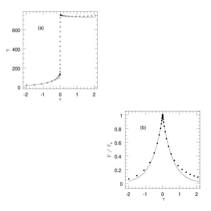
The numerical results for the temperature and flux in a subcritical shock wave ( km/sec) are plotted as a function of the compression ratio (Fig. 2) and optical depth from the shock front (Fig. 4). In these plots, we have scaled the temperatures to and the flux to . The gas pressure is plotted as a function of the compression ratio in Fig. 3. In each plot, we have superposed the appropriate analytic solution (see §2.3).
The adaptive grid has concentrated a large number of points in the shock front and the structure of the front is well resolved. Each point in Figs. 2 and 3 represents a single fluid element. The effective resolution near the shock front exceeds , i.e., by incorporating adaptive grid with points we reach a resolution which is equivalent to a fixed grid with points.
The analytic and numerical solutions agree very well in both the shocked material () and in the preheated gas (). The analytic solution correctly links the initial and final states of the gas, but it slightly underestimates (Fig. 2). The gas pressure is a linear function of outside of the shock front, as predicted by eq. 2.3, and each fluid element follows an approximate Hugoniot curve through the shock front (Fig. 3). The radiation flux is constant through the shock front and viscous heating in the front raises the gas temperature. The maximum compression ratio observed in the shock is , so we have not quite reached the strong shock limit of .
Although compressional heating is about 50% larger than the change in the kinetic energy of the inflowing gas, because terms which are second order in are not negligibly small, this has a small effect on the structure of the shock wave. There are three, not entirely independent, reasons for this. First, compressional heating of the gas does not change the temperature of the gas by a large amount. In Fig. 4a, it is clear that declines nearly exponentially with optical depth from the shock, as expected for radiative cooling. Second, radiative heating and cooling change the gas temperature near the shock by of . This minimizes the consequences of the assumed relation (eq. 13). Third, the radiative transfer equation is independent of the gas temperature because the radiation energy density is much larger than the equilibrium value of .
When the radiation energy density , the radiation flux falls exponentially with increasing optical depth from the shock discontinuity. The numerical solution for , scaled to the flux at the discontinuity, is plotted with the analytic approximation in Fig. 4b. The agreement between the two solutions is quite good for , where the radiation energy density is much larger than the equilibrium value. At larger , the radiation energy density approaches the equilibrium value and no longer falls exponentially. In this region, we find that the analytic estimate underestimates the true flux.
3.2 The Supercritical Shock Wave
The shock wave becomes supercritical when km/sec. The analytic estimate (eqs. 10 and 19) predicts that when km/sec, which is reasonably close to the numerical value. In the following, we use a run with km/sec to illustrate the structure of the supercritical shock wave. The structure of the shock front is illustrated with plots of the physical variables as functions of (Figs. 5 and 6) and (Fig. 7).
The conservation relations (eq. 2.3) accurately link the initial and final states of the gas (Fig. 5). The numerical solution reproduces the isothermal profile of the shocked gas and the linear dependence of on downstream from the discontinuity. No net energy leaves the system, so the temperature of the shocked gas is given by eq. 10. Although the agreement between the numerical and analytic solutions is quite good downstream, the two solutions differ appreciably in the preheated gas.
We find that the gas temperature, pressure and radiation flux in the preheated gas is larger than predicted by the analytic solution of Zeldovich and Raizer (1967). There are two reasons for the discrepancy. First, the terms proportional to are not vanishingly small. Physically, this means that the compressional work done on the inflow is larger than the change in the kinetic energy of the gas. This results in more heating of the gas. Second, the analytic solution underestimates the radiation flux in the preheated gas (see Figs. 5 and 7), particularly within a few radiation mean free paths of the optically thin temperature spike. The additional radiation flux contributes to the local heating rate. Both effects tend to raise the gas temperature. When , and the second order terms are smaller, we find that the compressional work on the gas is very nearly equal to the change in the kinetic energy and the analytic solution for the gas temperature is much closer to the numerical result. However, the radiation flux remains larger than the analytic prediction. We attribute this to the additional flux from the optically thin spike.
The temperature profile of the optically thin temperature spike is determined by the balance of viscous heating and radiative cooling. In Fig. 5, the region between and corresponds to the optically thin temperature spike. Viscous heating raises the gas temperature from to and the gas cools radiatively at smaller (Fig. 5). We use in these simulations, so eq. 23 predicts , which is quite close to the numerical value of . The Zel’dovich and Raizer (1967) expression, , predicts , which is significantly less accurate than eq. 23. The two expressions agree within a few percent when so the distinction between the two expressions is unimportant in that case.
The area under the optically thin temperature spike must be conserved, so the height of the spike is determined by the (artificial) viscous heating length and the radiative cooling length. In Fig. 7b, we have plotted a detailed example of the temperature spike. It is clear that the width of the spike is determined by the radiative cooling length, which implies that the height of the spike does not depend upon the coefficient of artificial viscosity. However, we were not able to verify that the height of the spike reaches a maximum (set by eq. 23) because we could not reduce the viscosity to an arbitrarily small value.
Most of the radiation flux is formed in the temperature spike. The flux increases from the downstream of the spike to its peak value, at the downstream side of the discontinuity. The optical depth of the spike is . The large negative temperature gradient on the downstream side of the shock front generates a small flux into (i.e., ) the shocked gas. This is not seen in the analytic solution, which assumes that the flux is continuous across the discontinuity.
The structure of the supercritical shock is more evident when plotted as a function of optical depth from the shock (Fig. 7). We find that the numerical solution exhibits the expected three zone structure. In Fig. 7a, we plot and the radiation temperature as functions of the optical depth from the discontinuity. The gas and radiation field are in equilibrium () from the shock surface to . The solid line in Fig. 7 represents the analytic solution for the equilibrium layer (eq. 20) with K and . Both the temperature profile and the value of are remarkably close to the estimates in §2.3. At larger , the radiation drops out of equilibrium and both the radiation flux and the gas temperature start to drop exponentially with optical depth.
The predicted optical depth of the temperature spike is . In Fig. 7, we plot the temperature over a smaller range of to illustrate the structure of the spike. The gas and radiation temperatures are out of equilibrium in the spike and we define the optical depth of the spike as range of for which . We find that , which is reasonably close to the analytic estimate, particularly when one considers the many approximations that are involved in making that estimate.
In Fig. 7c), we plot the numerically determined radiation flux, scaled to the estimated peak flux (). It is clear that the analytic estimate is about 30% smaller than the actual peak flux. The approximate energy conservation relation (eq. 13) implies that in the preheated gas, and we find that this is very nearly satisfied. The exponential fall-off at is also verified.
3.3 Angular Distribution of the Radiation
Radiation from the subcritical shock is isotropic downstream from the shock () and rapidly approaches the free streaming value of upstream from the shock. The Eddington factors dip below 1/3 at the shock front, indicating that the radiation is preferentially emitted parallel to the shock front. This is because radiant energy generation occurs primarily in a thin shell, approximately a radiation mean free path across, at the shock radius (eq. 18). Rays which are nearly parallel to the shock front have a larger path length for energy generation and the flux along these directions is correspondingly enhanced.
The radiation from the supercritical shock remains isotropic from the piston to the outer edge of the equilibrium region (Fig. 9). The Eddington factors again fall below 1/3 at the shock radius, for the reasons just discussed, but in the supercritical case the range of radii for which is smaller. This is because the temperature spike at the shock radius is much thinner, , than in the subcritical shock (eq. 24). At large radii, the gas becomes optically thin and the Eddington factors approach the free streaming value of 1.
3.4 Effects of the Assumed Radiation Transport Mechanism
The diffusion approximation (e.g., Mihalas and Mihalas 1978) is often used to simplify the radiative transfer moment equations (eqs. 3 and 5). In place of the radiation momentum equation (eq. 3), one assumes that the radiation flux is proportional to the gradient of the radiation energy density
| (26) |
This is equivalent to assuming that the gas is optically thick and isotropic, i.e., . If the diffusion approximation is invoked, the equation for the radiation momentum (eq. 26) is no longer explicitly time dependent.
There are two variants of this approximation – equilibrium and non-equilibrium diffusion. The gas and radiation temperatures are assumed to be the same in equilibrium diffusion. This is a reasonable approximation if the time and length scales for energy exchange between the gas and the radiation field are shorter than any scale in the flow. In the non-equilibrium diffusion approximation, the radiation energy density, and , is determined by the radiation energy equation (eq. 5).
We find that non-equilibrium diffusion is a good approximation to the full radiation transport scheme (Fig. 10). The gas is optically thick over most of the flow and the radiation is nearly isotropic in all cases (see Figs. 8 and 9). The largest departures from isotropy occur at the shock front (§3.3) but even there they are fairly small. The smallest value of the Eddington factor in the shock front is .
Equilibrium diffusion is a reasonable approximation outside of the shock front but it breaks down inside the front (Fig. 10). The temperature gradient is very large in the shock and the temperature changes on scales much shorter than a photon mean free path. Thus, the radiation is out of equilibrium in the front (see Fig. 7b). Diffusion of radiation energy, caused by the assumption , artificially equalizes the gas temperature on either side of the shock () and the solution follows a path of constant temperature through the shock front. In the subcritical shock, this reduces and raises , relative to the full transport solution. Assuming equilibrium diffusion can cause one to overestimate by a factor of 3-4 (Fig. 10). In addition, in the shock is overestimated by a similar factor because the flux is assumed to be proportional to the temperature gradient. Equilibrium diffusion gives an accurate estimate of for a supercritical shock, but the extra energy diffusion erases the most distinctive feature of the shock, the temperature spike.
3.5 Relations between Upstream and Downstream Quantities
The post-shock gas temperature () increases nearly linearly with increasing . For a subcritical shock, the temperature of the shocked gas is related to the temperature of the preheated gas by eq. 15, and
| (27) |
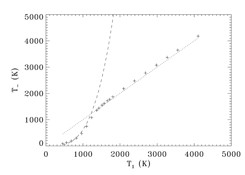
in a gas. We find that this solution is a good approximation to the numerical solution at . Above this temperature the shock becomes supercritical and , as predicted by eq. 23. In Figure 11, we have plotted the numerical results for several runs of increasing shock strength (crosses), the relation (short dashed line) and the Zel’dovich and Raizer (1967) relation . The two analytic expressions apply to a supercritical shock and the Zel’dovich and Raizer (1967) relation underestimates by about 10% in all cases. We find that eq. 23 is a much better description of the numerical solution.
Preheating raises the gas temperature ahead of the shock. We find that (the dashed line in Fig. 12) in a subcritical shock wave, as discused in §2.3. At supercritical shock strengths within a few percent. The temperature at which the shock makes the transition from subcritical to supercritical () can be estimated as the value of where the two approximate relations intersect. We find that , in reasonable agreement with the estimates in §2.3 and §3.2.
4 Conclusions
We have solved the time-dependent spherically symmetric equations of radiation hydrodynamics on an adaptive grid for both subcritical and supercritical radiating shock waves. In this paper, the shock wave is created by a supersonic piston moving into a shell of cold gas with a constant density. The gas opacity was assumed to be constant and purely absorptive. The shock propagates into the gas at a speed , where is the compression ratio just downstream of the shock front, and we find that the structure of the shock becomes steady in the shock frame after a time short compared to the flow time. The temperature of the shocked gas is approximately K, where is the piston speed in cm/sec.
The addition of the adaptive grid equation enables the code to fully resolve the radiating shock, so no jump conditions need to be employed and the effects of artificial viscosity are greatly reduced. The code achieved a peak resolution in the shock front of with 100 grid points. Thus, the grid resolves physical processes occurring on length scales over times smaller than the best fixed grid scheme.
The shock wave is subcritical when km/sec. The Zel’dovich and Raizer (1967) analytic solution for the gas temperature and radiation flux as a function of the compression ratio agrees with the numerical solution outside of the shock front. A single fluid element passes through the shock on an approximate Hugoniot curve and the radiation flux is constant, and the gas temperature increases, along this curve.
The radiation flux from a subcritical shock wave peaks at the shock radius and declines in proportion to , where is the optical depth of the gas measured relative to the shock front, when . At larger optical depths the radiation energy density approaches its equilibrium value and the actual flux falls less rapidly than the analytic model predicts. The Eddington factors are less than 1/3 at the shock front, indicating that the radiation is directed parallel to the shock.
The numerical solution for the supercritical shock wave ( km/sec) exhibits the expected three zone structure: shock heated gas at , an optically thin temperature spike at the gas pressure discontinuity and preheated gas in equilibrium with the radiation field (Zel’dovich and Raizer 1967). We find that the amplitude of the temperature spike is . The radiative cooling length in the spike is much shorter than the scale of the flow, so the adaptive grid must be used to resolve the spike. Fixed grid methods and equilibrium radiation diffusion introduce too much energy diffusion and the spike disappears from the numerical solution. Heating by the radiation from the shock heats gas ahead of the shock to . The radiation energy density remains near its equilibrium value, and , until , where is measured relative to the shock front. In this region, the gas temperature is roughly , in agreement with the analytic approximation (Zel’dovich and Raizer 1967).
Although the jump conditions correctly link the initial and final states of the gas, the analytic solution underestimates the gas temperature, pressure and the radiative flux. Optically thin emission from the spike, not included in the analytic solution, increases the radiation flux near the shock. In addition, the analytic solution assumes that the compressional work done on the flow is exactly equal to the change in the kinetic energy of the gas. We find that the compression work is typically larger than the change in kinetic energy and the discrepancy increases with . Both effects raise the temperature of the preheated gas.
References
- (1) Dorfi EA, Drury LO’C (1987) Simple adaptive grids for 1D initial value problems. J. Comp. Physics 69:175-195
- (2) Gehmeyr M, Mihalas D (1994) Adaptive grid radiation hydrodynamics with TITAN. Physica D 72:320-???
- (3) Heaslett MA, Baldwin BS (1963) Predictions of the structure of radiation-resisted shock waves. Phys. Fluids 6:781-791
- (4) Mihalas D, Mihalas BW (1984) Foundations of Radiation Hydrodynamics, Oxford University Press, Oxford
- (5) Tscharnuter WM, Winkler KH (1979) A method for computing selfgravitating gas flows with radiation. Comput. Phys. Commun. 18:171
- (6) Winkler KH, Norman ML, Mihalas D (1984) Adaptive mesh radiation hydrodynamics–I. The radiation transport equation in a completely adaptive coordinate system. J.Q.R.S.T. 31:473-478
- (7) Zel’dovich YB, Raizer YP (1967) Physics of Shock Waves and High Temperature Hydrodynamic Phenomena, Academic Press, New York
- (8)
Figure Captions
Figure 1. The structure of a subcritical (a) and a supercritical (b) radiating shock wave.
Figure 2. Gas temperature (upper curve) and radiation flux (lower curve) as a function of compression ratio (). The solid curves are the analytic expressions from ZR and the crosses are the numerical solution. Note that in this figure we plot (-).
Figure 3. Gas pressure as a function of compression ratio. The solid line is the analytic expression from ZR and the dashed line is the numerical result.
Figure 4. Gas temperature (a) and radiation flux (b) as a function of optical depth for a subcritical shock. The solid lines represent the analytic solution from ZR and the points are the numerical result.
Figure 5. The gas temperature and radiation as a function of compression ratio for a supercritical shock wave.
Figure 6. The gas pressure as a function of compression ratio for a supercritical shock wave.
Figure 7. Gas temperature (triangles) and radiation temperature (squares) as a function of optical depth for a supercritical shock (a). The temperature profile is shown for a small range of in (b). The radiation flux profile is plotted in (c). The solid curves are the analytic approximation for the temperature in the equilibrium zone.
Figure 8. Eddington factors as a function of optical depth for a subcritical shock. Note that at the shock radius.
Figure 9. Eddington factors as a function of optical depth for a supercritical shock. Note that at the shock radius.
Figure 10. The numerical solutions for full transport (crosses), non-equilibrium diffusion (open squares) and equilibrium diffusion (stars). The curve represents the analytic solution. The piston speeds are, from top to bottom: 12, 9 and 6 km/sec.
Figure 11. The post-shock gas temperature () as a function of the final temperature of the shocked gas.
Figure 12. The pre-shock gas temperature () as a function of the final temperature of the shocked gas.
Figure 13. The gas temperature as a function of the optical depth. Color coding is described in the appendix.
Figure 14. The gas pressure as a function of the optical depth. Color coding is described in the appendix.
Figure 15. The radiation flux as a function of the optical depth. Color coding is described in the appendix.
Figure 16. The Eddington factors as a function of the optical depth. Color coding is described in the appendix.