CMB POLARIZATION EXPERIMENTS Matias Zaldarriaga Department of Physics, MIT, Cambridge, MA 02139 USA

We discuss the analysis of polarization experiments with particular emphasis on those that measure the Stokes parameters on a ring on the sky. We discuss the ability of these experiments to separate the $E$ and $B$ contributions to the polarization signal. The experiment being developed at Wisconsin university is studied in detail, it will be sensitive to both Stokes parameters and will concentrate on large scale polarization, scanning a $43^{o}$ degree ring. We will also consider another example, an experiment that measures one of the Stokes parameters in a $1^{o}$ ring. We find that the small ring experiment will be able to detect cosmological polarization for some models consistent with the current temperature anisotropy data, for reasonable integration times. In most cosmological models large scale polarization is too small to be detected by the Wisconsin experiment, but because both $Q$ and $U$ are measured, separate constraints can be set on $E$ and $B$ polarization.

PACS numbers: 98.80.-k, 98.70.Vc, 98.80.Es

1 Introduction

Temperature anisotropies in the cosmic microwave background (CMB) can be considered one of the best probes of the early universe. The higher precision measurements that will become available in the near future could potentially lead to a precise determination of a large number of cosmological parameters [1, 2]. But the temperature anisotropies are not the only source of information, Thomson scattering of the CMB photons will lead to a small degree of linear polarization at a level detectable by the future generation of experiments.

The detection of polarization will provide information about our universe that is not available in the temperature data. For example it can provide an accurate determination of the ionization history of the universe [3]. Gravitational waves and vector modes also leave a specific signature in the polarization [4, 5]. The correlation function of the Stokes parameters $Q$ and $U$ can be used to test the causal structure of our Universe and thus provides a direct test of inflation [6]. The polarization power spectra produced by the current family of topological defect models are also very different from that produced by inflationary models [7].

The two future satellite missions, MAP and PLANCK, will measure polarization as well as temperature anisotropies. The extra information in polarization will help improve the constraints these missions can put on cosmological parameters [1]. For most parameters the expected error bars decrease by a factor of two and for those related to the reionization history of the universe the accuracy can be several times better.

Several ground based polarization experiments are now also under way. Some of these experiments plan to measure the Stokes parameters in pixels on a ring around the north celestial pole, which simplifies the pointing of the telescope. The properties of the experiment being developed at Wisconsin University [8] are discussed in detail. This experiment will concentrate on large angular scale polarization measuring both $Q$ and $U$ in a $43^{o}$ ring. We also consider another example, an experiment that measures only one Stokes parameter in a $1^{o}$ ring.

Recent theoretical developments [4, 5] have shown that rather than describing polarization in terms of $Q$ and $U$ it is more natural to introduce two scalar quantities $E$ and $B$. The correlation functions of this variables is what theories most easily predict and the treatment in terms of $E$ and $B$ takes full account of the spin $2$ nature of polarization.

The ring like polarization experiments appear as an ideal testing ground for this new formalism because they are being performed right now and also because their simple geometry will enable us to study them in full detail and build intuition on this new polarization formalism. We will study for example how this kind of experiments can separate the two components of polarization $E$ and $B$. Our treatment will also permit us to explore how changes of the experimental set up, like a change of the ring size, affect the experiments ability to detect cosmological polarization.

The outline of the paper is the following: in §2 we review previous results on polarization and describe the way in which general polarization experiments can be analyzed. In §3 we discuss specific properties of the ring like experiments and in §4 we study parameter estimation issues in the context of this kind of experiments. We make a summary and discuss our results in §5.

2 Correlation Functions

The CMB radiation field is described by a $2\,\times\,2$ intensity tensor $I_{ij}$ [9]. The Stokes parameters $Q$ and $U$ are defined as $Q=(I_{11}-I_{22})/4$ and $U=I_{12}/2$, while the temperature anisotropy is given by $T=(I_{11}+I_{22})/4$. The fourth Stokes parameter $V$ that describes circular polarization is not necessary in standard cosmological models because it cannot be generated through the process of Thomson scattering. While the temperature is a scalar quantity $Q$ and $U$ are not. They depend on the direction of observation $\hat{n}$ and on the two axis $(\hat{e}_{1},\hat{e}_{2})$ perpendicular to $\hat{n}$ used to define them. If for a given $\hat{n}$ the axes $(\hat{e}_{1},\hat{e}_{2})$ are rotated by an angle $\psi$ such that ${\hat{e}_{1}}^{\prime}=\cos\psi\ {\hat{e}_{1}}+\sin\psi\ {\hat{e}_{2}}$ and ${\hat{e}_{2}}^{\prime}=-\sin\psi\ {\hat{e}_{1}}+\cos\psi\ {\hat{e}_{2}}$ the Stokes parameters change as

$$Q^{\prime} = \cos 2\psi\ Q+\sin 2\psi\ U$$

$$U^{\prime} = -\sin 2\psi\ Q+\cos 2\psi\ U$$ (1)

To analize the CMB temperature on the sky it is natural to expand it in spherical harmonics. These are not appropriate for polarization, because the two combinations $Q\pm iU$ are quantities of spin $\pm 2$ [10]. They should be expanded in spin-weighted harmonics $\,{}_{\pm 2}Y_{l}^{m}$ [4],

$$T(\hat{n}) = \sum_{lm}a_{T,lm}Y_{lm}(\hat{n})$$

$$(Q+iU)(\hat{n}) = \sum_{lm}a_{2,lm}\;{}_{2}Y_{lm}(\hat{n})$$

$$(Q-iU)(\hat{n}) = \sum_{lm}a_{-2,lm}\;{}_{-2}Y_{lm}(\hat{n}).$$ (2)

To perform this expansion, $Q$ and $U$ in equation (2) are measured relative to $(\hat{e}_{1},\hat{e}_{2})=(\hat{e}_{\theta},\hat{e}_{\phi})$, the unit vectors of the spherical coordinate system. There is an equivalent expansion using tensors on the sphere [5]. The coefficients ${}_{\pm 2}a_{lm}$ are observable on the sky and their power spectra can be predicted for different cosmological models. Instead of ${}_{\pm 2}a_{lm}$ it is convenient to use their linear combinations $a_{E,lm}=-(a_{2,lm}+a_{-2,lm})/2$ and $a_{B,lm}=-(a_{2,lm}-a_{-2,lm})/2i$, which transform differently under parity. Four power spectra are needed to characterize fluctuations in a gaussian theory, the autocorrelation between $T$, $E$ and $B$ and the cross correlation of $E$ and $T$. Because of parity considerations the cross-correlations between $B$ and the other quantities vanish and one is left with

$$\langle a_{X,lm}^{*}a_{X,lm^{\prime}}\rangle = \delta_{m,m^{\prime}}C_{Xl}$$

$$\langle a_{T,lm}^{*}a_{E,lm}\rangle = \delta_{m,m^{\prime}}C_{Cl},$$ (3)

where $X$ stands for $T$, $E$ or $B$, $\langle\cdots\rangle$ means ensemble average and $\delta_{i,j}$ is the Kronecker delta.

For the purpose of this work it is more useful to rewrite equation (2) as

$$T(\hat{n}) = \sum_{lm}a_{T,lm}Y_{lm}(\hat{n})$$

$$Q(\hat{n}) = -\sum_{lm}a_{E,lm}X_{1,lm}+ia_{B,lm}X_{2,lm}$$

$$U(\hat{n}) = -\sum_{lm}a_{B,lm}X_{1,lm}-ia_{E,lm}X_{2,lm}$$ (4)

where we have introduced $X_{1,lm}(\hat{n})=(\;_{2}Y_{lm}+\;_{-2}Y_{lm})/2$ and $X_{2,lm}(\hat{n})=(\;_{2}Y_{lm}-\;_{-2}Y_{lm})/2$. They satisfy $X^{*}_{1,lm}=X_{1,l-m}$ and $X^{*}_{2,lm}=-X_{2,l-m}$ which together with $a_{E,lm}=a_{E,l-m}^{*}$ and $a_{B,lm}=a_{B,l-m}^{*}$ make $Q$ and $U$ real.

In fact $X_{1,lm}(\hat{n})$ and $X_{2,lm}(\hat{n})$ have the form, $X_{1,lm}(\hat{n})=\sqrt{(2l+1)/4\pi}$ $F_{1,lm}(\theta)\ e^{im\phi}$ and $X_{2,lm}(\hat{n})=\sqrt{(2l+1)/4\pi}$ $F_{2,lm}(\theta)\ e^{im\phi}$, $F_{(1,2),lm}(\theta)$ can be calculated in terms of Legendre polynomials [5] :

$$F_{1,lm}(\theta) = 2\sqrt{(l-2)!(l-m)!\over(l+2)!(l+m)!}[-({l-m^{2}\over\sin^{2}\theta}+{1\over 2}l(l-1))P_{l}^{m}(\cos\theta)$$

$$+(l+m){\cos\theta\over\sin^{2}\theta}P_{l-1}^{m}(\cos\theta)]$$

$$F_{2,lm}(\theta) = 2\sqrt{(l-2)!(l-m)!\over(l+2)!(l+m)!}{m\over\sin^{2}\theta}[-(l-1)\cos\theta P_{l}^{m}(\cos\theta)$$ (5)

$$+(l+m)P_{l-1}^{m}(\cos\theta)].$$

Note that $F_{2,lm}(\theta)=0$ if $m=0$, as it must to make the Stokes parameters real.

The correlation functions can be calculated using equations (3) and (4),

$$\langle T(1)T(2)\rangle = \sum_{l}C_{Tl}[\sum_{m}\;{}_{0}Y_{lm}^{*}(1)\;_{0}Y_{lm}(2)]$$

$$\langle Q(1)Q(2)\rangle = \sum_{l}C_{El}[\sum_{m}X_{1,lm}^{*}(1)X_{1,lm}(2)]+C_{Bl}[\sum_{m}X_{2,lm}^{*}(1)X_{2,lm}(2)]$$

$$\langle U(1)U(2)\rangle = \sum_{l}C_{El}[\sum_{m}X_{2,lm}^{*}(1)X_{2,lm}(2)]+C_{Bl}[\sum_{m}X_{1,lm}^{*}(1)X_{1,lm}(2)]$$

$$\langle T(1)Q(2)\rangle = \sum_{l}C_{Cl}[\sum_{m}\;{}_{0}Y_{lm}^{*}(1)X_{1,lm}(2)]$$

$$\langle T(1)U(2)\rangle = i\sum_{l}C_{Cl}[\sum_{m}\;{}_{0}Y_{lm}^{*}(1)X_{2,lm}(2)]$$ (6)

where $1$ and $2$ stand for the two directions in the sky $\hat{n}_{1}$ and $\hat{n}_{2}$. These expressions can be further simplified using the addition theorem for the spin harmonics [11],

$$\sum_{m}\;{}_{s_{1}}Y_{lm}^{*}(\hat{n}_{1})\;_{s_{2}}Y_{lm}(\hat{n}_{2})=\sqrt{2l+1\over 4\pi}\;_{s_{2}}Y_{l-s_{1}}(\beta,\psi_{1})e^{-is_{2}\psi_{2}}$$ (7)

where $\beta$ is the angle between $\hat{n}_{1}$ and $\hat{n}_{2}$, and $(\psi_{1}$,$\psi_{2})$ are the angles $(\hat{e}_{\theta},\hat{e}_{\phi})$ at $\hat{n}_{1}$ and $\hat{n}_{2}$ need to be rotated to become aligned with the great circle going through both points. In the case of the temperature equation(7) gives the usual relation,

$$\langle T_{1}T_{2}\rangle=\sum_{l}{2l+1\over 4\pi}C_{Tl}P_{l}(\cos\beta).$$ (8)

For polarization the addition relations for $X_{1,lm}$ and $X_{2,lm}$ are calculated from equation (7),

$$\sum_{m}X_{1,lm}^{*}(1)X_{1,lm}(2) = {2l+1\over 4\pi}[F_{1,l2}(\beta)\cos 2\psi_{1}\cos 2\psi_{2}-F_{2,l2}(\beta)\sin 2\psi_{1}\sin 2\psi_{2}]$$

$$\sum_{m}X_{2,lm}^{*}(1)X_{2,lm}(2) = {2l+1\over 4\pi}[F_{1,l2}(\beta)\sin 2\psi_{1}\sin 2\psi_{2}-F_{2,l2}(\beta)\cos 2\psi_{1}\cos 2\psi_{2}]$$

$$\sum_{m}X_{1,lm}^{*}(1)X_{2,lm}(2) = i{2l+1\over 4\pi}[F_{1,l2}(\beta)\sin 2\psi_{1}\cos 2\psi_{2}+F_{2,l2}(\beta)\cos 2\psi_{1}\sin 2\psi_{2}]$$

$$\sum_{m}\;{}_{0}Y_{lm}^{*}(1)X_{1,lm}(2) = {2l+1\over 4\pi}F_{1,l0}(\beta)\cos 2\psi_{2}$$

$$\sum_{m}\;{}_{0}Y_{lm}^{*}(1)X_{1,lm}(2) = -i{2l+1\over 4\pi}F_{1,l0}(\beta)\sin 2\psi_{2}$$ (9)

where we can equivalently write $F_{1,l0}(\beta)=\sqrt{(l-2)!/(l+2)!}P_{l}^{2}(\beta)$.

The correlations in equation (6) with the sums given by equation (9) are all what is needed to analize any given experiment. These relations are simple to understand, as pointed out in [5] the natural coordinate system to express the correlations is one in which both $(\hat{e}_{1},\hat{e}_{2})$ reference frames are chosen to be aligned with the great circle connecting the two directions (1 and 2); in that case we have [5]

$$\langle Q_{r}(1)Q_{r}(2)\rangle = \sum_{l}{2l+1\over 4\pi}[C_{El}F_{1,l2}(\beta)-C_{Bl}F_{2,l2}(\beta)]$$

$$\langle U_{r}(1)U_{r}(2)\rangle = \sum_{l}{2l+1\over 4\pi}[C_{Bl}F_{1,l2}(\beta)-C_{El}F_{2,l2}(\beta)]$$

$$\langle T(1)Q_{r}(2)\rangle = \sum_{l}{2l+1\over 4\pi}C_{Cl}F_{1,l0}(\beta)$$

$$\langle T(1)U_{r}(2)\rangle = 0$$ (10)

the subscript $r$ here indicate that the Stokes parameters are measured in this particular coordinate system. We can use the transformation laws in equation (1) to write $(Q,U)$ in terms of $(Q_{r},U_{r})$ and then using equation (10) for their correlations one can recover our final result (given by equations (6) and (9)).

When analyzing an experiment we can arrange the measured values of $T$, $Q$ and $U$ in a vector ${\bf x}=(T_{1},Q_{1},U_{1},...T_{i},Q_{i},U_{i}...)$, the subscript labels the pixel. The measured Stokes parameters at each pixel have two contributions, the first coming from the cosmological signal we are interested in measuring, given by equation (4) and the second from the noise in the detectors. The correlation matrix of ${\bf x}$ is $\langle{\bf x}_{i}{\bf x}_{j}\rangle\equiv{\bf C}_{ij}={\bf S}_{ij}+{\bf N}_{ij}$, where the signal correlation matrix ${\bf S}$ is given in equations (6) and (9) and ${\bf N}$ is the correlation matrix of the noise. With this correlation matrix the full likelihood can be calculated,

$$L({\bf x}|C_{Xl})\propto{1\over\sqrt{\det C}}\exp[-{1\over 2}{\bf x}^{T}{\bf C}^{-1}{\bf x}],$$ (11)

here $C_{Xl}$ stands for the complete set of power spectra that describe the theory under consideration, $C_{Xl}=\{C_{Tl},C_{El},C_{Bl},C_{Cl}\}$. If the set of power spectra are given in terms of a set of parameters, the likelihood can be maximized to find parameters that best fit the data.

3 Ring Experiments

There are several ground based polarization experiments now under way. Some of these experiments plan to measure the Stokes parameters $Q$ and $U$ in pixels that form a ring on the sky. The simple geometry of the sky patch is perfect for understanding the relation between $E$ and $B$ polarization and the Stokes parameters. It is the aim of this section to analyze this kind of experiments.

Rather than doing the analysis in terms of correlations in real space as was suggested in the previous section, in this case it is simple to diagonalize the signal correlation matrix. If the noise is uncorrelated and equal from pixel to pixel (ie. the noise correlation matrix is proportional to the identity matrix) we simultaneously diagonalize the noise and signal correlation matrices. This will allow us to make a more detailed analysis of the characteristics of this type of experiments.

Let us assume that the experiment measures the Stokes parameters in a number ($N_{pix}$) of pixels on a ring of radius $\theta$ with a gaussian beam of width $\theta_{fwhm}$. We will take the noise correlation matrix to be diagonal, $\langle{N}_{(Q,U)i}{N}_{(Q,U)j}\rangle=\sigma_{P}^{2}\delta_{ij}$ and uncorrelated between $Q$ and $U$, ${N}_{(Q,U)j}$ are the noise contribution to the measured $Q$ and $U$ in pixel $j$. If $\phi_{j}=2\pi(j-1)/N_{pix}$ denotes the angle along the ring, the Stokes parameters in each pixel are given by (equation (4) plus the noise contribution)

$$Q_{j} = -\sum_{lm}\sqrt{(2l+1)/4\pi}B_{lm}[a_{E,lm}F_{1,lm}(\theta)$$

$$+ia_{B,lm}F_{2,lm}(\theta)]e^{im\phi_{j}}+N_{Qj}$$

$$U_{j} = -\sum_{lm}\sqrt{(2l+1)/4\pi}B_{lm}[a_{B,lm}F_{1,lm}(\theta)$$ (12)

$$-ia_{E,lm}F_{2,lm}(\theta)]e^{im\phi_{j}}+N_{Uj},$$

here $B_{lm}$ encodes the information the beam and scan pattern of the experiment. In an appendix we make the derivation of these functions for the Wisconsin experiment. In what follows we will take $B_{lm}^{2}=\exp{[-l(l+1)\sigma_{b}^{2}]}$ with $\sigma_{b}=\theta_{fwhm}/2\sqrt{2\ln 2}$ which is a good first approximation.

Diagonalizing the signal correlation matrix is very simple and intuitive: if one considers the Fourier transform of the data then each mode will pick a particular value of $m$ in equation (12). In particular let us consider the transformed data set

$${\bar{Q}}^{k} \equiv {1\over N_{pix}}\sum_{j}Q_{j}e^{-ik\phi_{j}}$$

$$= -\sum_{l\geq|k|}\sqrt{(2l+1)/4\pi}B_{lk}[a_{E,lk}F_{lk}^{1}(\theta)+ia_{B,lk}F_{lk}^{2}(\theta)]+{\bar{N}}_{Q}^{k}$$

$${\bar{U}}^{k} \equiv {1\over N_{pix}}\sum_{j}U_{j}e^{-ik\phi_{j}}$$ (13)

$$= -\sum_{l\geq|k|}\sqrt{(2l+1)/4\pi}B_{lk}[a_{B,lk}F_{lk}^{1}(\theta)-ia_{E,lk}F_{lk}^{2}(\theta)]+{\bar{N}}_{U}^{k}$$

where $k$ runs from $-N_{pix}/2\leq k\leq N_{pix}/2$. To get to the last expression we have used that,

$$\sum_{j=1}^{N_{pix}}e^{i(m-k)\phi_{j}} = \sum_{j=0}^{N_{pix}-1}(e^{i(m-k)2\pi/N_{P}ix})^{j}$$ (14)

$$= (1-e^{i(m-k)2\pi})/(1-e^{i(m-k)2\pi/N_{pix}})$$

$$= N_{pix}\delta_{m,k+nN_{pix}}$$

where $n$ is any integer. The sum in equation (14) is only different from zero if $k=m$ or if it differs by a multiple of $N_{pix}$. To obtain equation (13) we ignored the terms that “leak” power from higher harmonics, only $k=m$ is considered. This is a reasonable assumption because higher harmonics are suppressed by beam smearing. In fact we should always choose $N_{pix}$ large enough so as to oversample the beam and not loose the information in the smaller scales, this immediately guaranties that the aliased power is negligible.

In equation (13) we have labeled the Fourier transforms of the noise contributions ${\bar{N}}_{(Q,U)}^{k}$ which under the assumption of uniform uncorrelated noise satisfies,

$$\langle{\bar{N}}_{Q}^{k*}{\bar{N}}_{Q}^{k^{\prime}}\rangle = w_{P}^{-1}\delta_{k,k^{\prime}}$$

$$\langle{\bar{N}}_{U}^{k*}{\bar{N}}_{U}^{k^{\prime}}\rangle = w_{P}^{-1}\delta_{k,k^{\prime}}$$

$$\langle{\bar{N}}_{Q}^{k*}{\bar{N}}_{U}^{k^{\prime}}\rangle = 0$$

$$\langle{\bar{N}}_{U}^{k*}{\bar{N}}_{Q}^{k^{\prime}}\rangle = 0$$ (15)

where $w^{-1}_{P}\equiv\sigma_{P}^{2}/N_{pix}$.

We will take the data set to be the Fourier coefficients rather than the Stokes parameters. The signal part of each Fourier component receives contributions only from multipoles with $m=k$, equation (3) then implies that only components with the same value of $k$ will be correlated. The correlation matrix is block diagonal,

$$\langle{\bar{Q}}^{k*}{\bar{Q}}^{k^{\prime}}\rangle = \delta_{k,k^{\prime}}\sum_{l\geq k}{(2l+1)/4\pi}B_{lk}^{2}[C_{E,l}F_{1,lk}^{2}(\theta)+C_{B,l}F_{2,lk}^{2}(\theta)]$$

$$+\delta_{k,k^{\prime}}w_{P}^{-1}$$

$$\langle{\bar{U}}^{k*}{\bar{U}}^{k^{\prime}}\rangle = \delta_{k,k^{\prime}}\sum_{l\geq k}{(2l+1)/4\pi}B_{lk}^{2}[C_{E,l}F_{2,lk}^{2}(\theta)+C_{B,l}F_{1,lk}^{2}(\theta)]$$

$$+\delta_{k,k^{\prime}}w_{P}^{-1}$$

$$\langle{\bar{U}}^{k*}{\bar{Q}}^{k^{\prime}}\rangle = \delta_{k,k^{\prime}}\sum_{l\geq k}i{(2l+1)/4\pi}B_{lk}^{2}(C_{E,l}+C_{B,l})F_{1,lk}(\theta)F_{2,lk}(\theta)$$

$$\langle{\bar{Q}}^{k*}{\bar{U}}^{k^{\prime}}\rangle = -\langle{\bar{U}}^{k*}{\bar{Q}}^{k^{\prime}}\rangle,$$ (16)

“$*$” means complex conjugate. An important point is that this transformation does not rely on the particular shape or other property of the power spectra, if the CMB is a statistically isotropic and homogeneous random field taking the Fourier transform will always make the correlation matrix block diagonal. The correlation matrix is hermitian, and the cross correlation between ${\bar{U}}^{k}$ and ${\bar{Q}}^{k^{\prime}}$ is imaginary. It will be more convenient to change variables and use $i{\bar{U}}^{k}\rightarrow{\bar{U}}^{k}$, the data set will then be ${\bf x}_{k}=({\bar{Q}}^{k},i{\bar{U}}^{k})$. The correlation matrix for each $k$ is given by equation (16) but without the $i$ in the cross term.

In the Fourier domain the likelihood becomes a product of independent gaussians, one for each $k$,

$$L({\bf x}|C_{Xl})\propto\prod_{k}{1\over\sqrt{\det C_{k}}}\exp[-{1\over 2}{\bf x}^{{\dagger}}_{k}{\bf C}_{k}{\bf x}_{k}],$$ (17)

where the ${\bf C}_{k}$ matrices are $2\times 2$ given by equation (16) and ${\dagger}$ means transpose and complex conjugate. Clearly if only one of the Stokes parameters is measured then the likelihood is just the product of several one dimensional gaussians and if the temperature is also included in the analysis ${\bf C}_{k}$ turns into a $3\times 3$ matrix.

Equation (16) shows that if a ring experiment only measures one of the Stokes parameters, either ${\bar{Q}}^{k}$ or ${\bar{U}}^{k}$ it will not be able to separate the $E$ and $B$ contributions in a model independent way because both contributions enter in the expressions summed together. This is similar to what happens if one is interested in separating the contributions from density perturbations and gravitational waves to the temperature anisotropies. It is only when one assumes a shape for the power spectra that one can fit the observed temperature spectra as a sum of these two separate contributions and infer the presence of gravity waves. In a similar way if we only measure ${\bar{Q}}^{k}$ and we assume different shapes for both $C_{El}$ and $C_{Bl}$ we could determine each contribution. On the other hand if both Stokes parameters are measured then we could separate the $E$ and $B$ contribution directly as they enter differently in each correlation (multiplied by $F_{1,lk}^{2}(\theta)$ and $F_{2,lk}^{2}(\theta)$ in $Q$ and the other way around in $U$).

Another interesting property of equation (16) is that the $k=0$ $Q$ mode does not receive any contribution from the $B$ channel because $F_{2,l0}(\theta)\equiv 0$, the converse is true for $U$. For example a non zero signal in ${\bar{U}}^{0}$ implies the presence of $B$ and thus of gravity waves or vector modes. Of course this determination suffers from a large cosmic variance, because we are only measuring one realization.

3.1 Small scale experiment

Let us now analize how the signal in each mode depends on the power spectrum. We will do this first for a small ring experiment that measures only $Q$ on a ring with $\theta=1^{o}$, $\theta_{fwhm}=0.22^{o}$. We selected a small ring scanned with a fraction of a degree resolution to make the experiment sensitive to small scale polarization. We will choose $w^{-1}_{P}=(0.9\mu K)^{2}$, corresponding to a receiver noise of $1.2mK/\sqrt{Hz}$ and three weeks of observations. This numbers are chosen to be representative of what a ground experiment might achieve.

The correlation matrix is

$$\langle{\bar{Q}}^{k*}{\bar{Q}}^{k^{\prime}}\rangle=\delta_{k,k^{\prime}}\sum_{l}{(2l+1)/4\pi}(W_{1,lk}C_{E,l}+W_{2,lk}C_{B,l})+\delta_{k,k^{\prime}}w^{-1}_{P}.$$ (18)

Both signal and noise parts are diagonal and we have introduced the window functions $W_{1,lk}=B_{lk}^{2}\ F_{1,lk}^{2}(\theta)$ and $W_{2,lk}=B_{lk}^{2}\ F_{2,lk}^{2}(\theta)$ which describe how each Fourier mode depends on the underlying power spectra. Let us consider what the experiment would measure if the underlying cosmological model was standard CDM. We will assume there are no gravity waves or vector modes so we will only consider $E$ type polarization. We will generalize our analysis later.

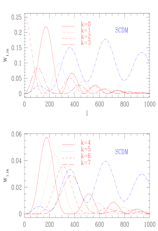
Figure 1: Window functions for the small ring experiment for several values of $k$. The SCDM spectrum is also shown for comparison, we actually plot $(l+1)C_{El}/2\pi$ which is the relevant measure of power for a linear $l$ scale (the normalization is arbitrary).

Figure 1 shows the window functions $W_{1,lk}$ for several values of $k$. Only multipoles $l\geq|k|$ contribute to Fourier component $k$. As $|k|$ grows the peaks of the window functions move to higher $l$ (we only show results for the $k>0$ modes but they also apply to the $k<0$ ones). The window functions are very broad in $l$ space, because their width is inversely proportional to the smallest dimension of the sky patch one is observing. For large values of $l$ the window functions are cut off by the effect of the beam smearing, $B^{2}_{lk}$.

Figure 1 also shows that the most important contribution to the signal in this experiment comes from the second polarization acoustic peak at $l\sim 350$, the first peak at $l\sim 100$ contributes to a smaller extent. Higher peaks are inaccessible because of beam smearing.

An interesting point to note is that the $k=2$ window function peaks at low $l$ (the lowest $l$ in the polarization expansion is by definition $l=2$), so it is this mode rather than $k=0$ or $1$ that gets the contribution from the largest angular scale perturbations. To understand why let us consider a small patch of the sky containing the $\theta=1^{o}$ ring and a polarization field that is constant over the patch. This polarization field is produced by the very large angular scale perturbations, the low $l$ modes. Without loss of generality let us call ${\hat{e}_{x}}$ the direction of the polarization vectors, ${\hat{e}_{y}}$ will be perpendicular to that. The Stokes parameters are measured relative to the $({\hat{e}_{\theta}},{\hat{e}_{\phi}})$ basis which rotates as one moves along the ring. Although the polarization amplitude $P$ is constant over the whole patch and the direction is always ${\hat{e}_{x}}$ the Stokes parameters along the ring (measured in the $({\hat{e}_{\theta}},{\hat{e}_{\phi}})$ basis) are given by

$$Q_{j} = P\cos 2\phi_{j}$$

$$U_{j} = P\sin 2\phi_{j},$$ (19)

and thus the $k=\pm 2$ Fourier modes will get all the signal. The coordinate system used to describe the Stokes parameters, which is rotating as one moves along the ring, and their spin 2 nature, which tells us how $Q$ and $U$ transform under this rotation, makes the large angular scale perturbations contribute only to the $k=\pm 2$ mode. This is another illustration of the spin 2 nature of polarization.

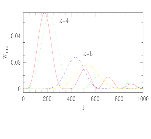
Figure 2: Window functions for the small ring experiment for $k=4,8$ and two ring sizes $\theta=1^{o},0.8^{o}$.

Another interesting thing to consider is the effect of the size of the ring on the window functions. The window functions are oscillating functions of $l$ and changes in the ring size modify the period of these oscillations. In particular the separation between peaks scales as $1/\theta$, and at the same time as the peaks become more separated they also become broader. This is most easily understood in the small scale limit. If we can neglect the curvature of the sky, which is an excellent approximation for this experiment, we can use Fourier transforms instead of spherical harmonics and write [12, 4]

$$Q({\bf\theta})=(2\pi)^{-2}\int d^{2}lE({\bf l})\cos 2(\phi-\phi_{l})\;e^{il\theta\cos(\phi-\phi_{l})}$$ (20)

where ${\bf\theta}$ labels the Fourier mode with $(l_{x}+il_{y})=l\exp{(i\phi_{l})}$. We have again considered only $E$ type polarization and here $\langle E({\bf l}_{1})E({\bf l}_{2})\rangle=C_{El_{1}}\delta^{D}({\bf l}_{2}-{\bf l}_{1})$, $\delta^{D}({\bf x})$ is the Dirac $\delta-$function. A straightforward calculation leads to

$${\bar{Q}}^{k}=-{1\over 2\pi}\int d^{2}lE({\bf l})e^{-ik\phi_{l}}\ {1\over 2}[J_{k+2}(u)+J_{k-2}(u)],$$ (21)

where $u=l\theta$ and $J_{n}(u)$ are Bessel functions. The correlation matrix is then given by

$$\langle{\bar{Q}}^{k*}{\bar{Q}}^{k^{\prime}}\rangle=\delta_{k,k^{\prime}}\int{ldl\over 2\pi}\ C_{El}\ {1\over 4}[J_{k+2}(u)+J_{k-2}(u)]^{2}$$ (22)

which means that the window function in the small scale limit is $W_{1,lk}={1\over 4}[J_{k+2}(u)+J_{k-2}(u)]^{2}$. The effect of changing the size of the ring is straight forward to understand in this expression, each $W_{1,lk}$ is only a function of $u=l\theta$ so changes in $\theta$ just cause a stretching of the window function. A similar analysis for the other set of window function yields $W_{2,lk}={1\over 4}[J_{k_{1}+2}(u)-J_{k_{1}-2}(u)]^{2}$. Beam smearing only adds a $B_{lk}^{2}$ to the expressions of both $W_{(1,2),lk}$ . Figure 2 shows two examples of these window functions for two ring sizes, the effect of scaling together with the $B_{lk}^{2}$ factor is clear.

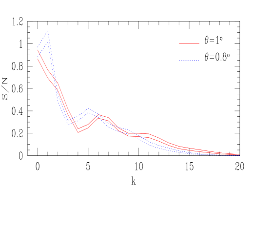
Figure 3: Signal to noise in the different modes for the small ring experiment assuming $w_{P}^{-1}=(0.9\mu K)^{2}$ and COBE normalized SCDM as the underlying model. Two different ring sizes are plotted, in each case the effect of changing the beam width from $0.22^{o}$(upper curve) to $0.2^{o}$ (lower curve) is also shown.

In figure 3 we show the S/N for each of the Fourier modes, that is the ratio of the signal to the noise part of the correlation in (equation 18), as a function of $k$. As expected the signal to noise decreases with increasing $k$ because of beam smearing. The effect of decreasing the ring size is evident in the figure, because the window functions for successive $k$ become more separated and at the same time broader the signal in the experiment gets concentrated in fewer Fourier modes. Also note that there is a peak at $k\sim 7$ when the ring is $\theta=1^{o}$ because this window function just matches the second acoustic peak and is then able to pick more power. The position of this peak is shifted to lower $k$ when the size of the ring is decreased.

It is important to recognize that most modes have a $S/N$ smaller than one, which will make the polarization hard to detect. Other models different from SCDM would produce a higher signal, but reducing the noise in the experiment would crucially improve its sensitivity to cosmological polarization. On the other hand the overall S/N of the experiment not just mode by mode is better, opening the possibility that cosmological polarization will be detected in the near future with this type of experiments.

3.2 Wisconsin experiment

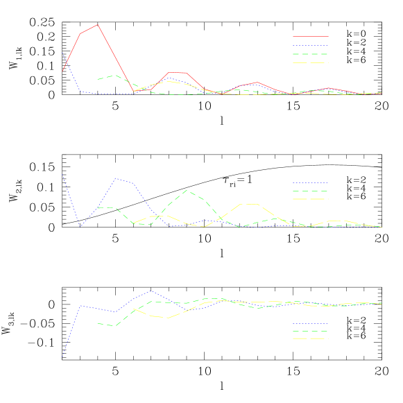
Figure 4: Window functions for the Wisconsin experiment for several values of $k$. For comparison in the middle pannel we show the $E$ spectra, $(l+1)C_{El}/2\pi$, for SCDM but with $\tau_{ri}=1$ (the normalization is arbitrary).

Let us now consider the Wisconsin experiment, because it will actually measure both $Q$ and $U$ on the ring it is in principle capable of distinguishing between $E$ and $B$ polarizations. The ring will be $\theta=43^{o}$, scanning the sky on the vertical at Wisconsin. It will have $\theta_{fwhm}=7^{o}$ and $w^{-1}_{P}=(0.4\mu K)^{2}$, the experiment is thus sensitive to large scale polarization. Unfortunately the large scale polarization is very small in most cosmological models for the sensitivity of this experiment.

Figure 4 shows some of the window functions for the experiment with $W_{1,lk}=B_{lk}^{2}\ F_{1,lk}^{2}(\theta)$, $W_{2,lk}=B_{lk}^{2}\ F_{2,lk}^{2}(\theta)$ and $W_{3,lk}=B_{lk}^{2}\ F_{1,lk}(\theta)\ F_{2,lk}(\theta)$. Note that the window functions for the cross correlation between $Q$ and $U$ can actually be negative. The properties of these window functions are the same as those discaused above for the small scale experiment, but note that because both the ring and the beam are much bigger now, the experiment is only sensitive to $l\leq 25$.

We will illustrate the features of this experiment by considering different underlying toy models, for simplicity we will take the power per logarithmic interval of $E$ and $B$ to be constant, $l(l+1)C_{(E,B),l}/2\pi=\sigma^{2}_{(E,B)}$. Figure 5 shows the $Q$ and $U$ $S/N$, the ratio of the signal to the noise contributions to the autocorrelations, for a model with $\sigma_{E}^{2}=2\mu K^{2}$ and no $B$. For comparison we also show what is expected for SCDM with an optical depth due to reionization $\tau_{ri}=1.0$. Note that even for this large optical depth the expected signal to noise is very small. The smaller $k$ modes have smaller S/N in the $\tau_{ri}=1$ model than in the flat spectra model because large scale polarization power spectra decreases rapidly with $l$ in all realistic models. In figure 4 we also show the $E$ spectra for a model with $\tau_{ri}=1$. All models where the universe reionizes at an early enough epoch have a peak in the large angular scale polarization spectra [3]. For this model $l_{peak}\sim 20$ and in general $l_{peak}\sim 2\sqrt{z_{ri}}$ with $z_{ri}$ the redshift at which the universe reionizes. We can see that the window function of the experiment are more sensitive to larger angular scale polarization and thus although the peak of the $\tau_{ri}=1$ model has an amplitude of $\sim 6\mu K^{2}$ the flat spectrum model with amplitude $2\mu K^{2}$ produces a higher S/N for most $k$.

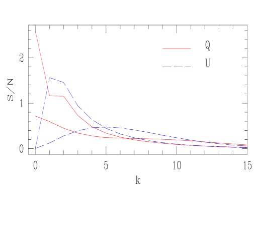
Figure 5: S/N for the Stokes parameters in the Wisconsin experiment. At low $k$ for both $Q$ and $U$ the lower curve corresponds to COBE normalized SCDM with $\tau_{ri}=1.0$, the upper curves are for a model with $\sigma_{E}^{2}=2\mu K^{2}$ and $\sigma_{B}^{2}=0\mu K^{2}$.

The experiment can only detect cosmological polarization for extreme models with a very early reionization. On the other hand it has the virtue of being able to put separate constraints on $E$ and $B$ because it measures both $Q$ and $U$. This is the feature of the experiment that we are most interested in. We will analyze simplified models with constant power spectrum for both $E$ and $B$. This will allow us to study what kind of constraints a ring experiment can put on $E$ and $B$ separately, not relying on the different shapes of these two contributions. The approximation also makes visualization of the results easier and it is also straight forward to get results for any other noise level, one just needs to rescale the values of $\sigma_{(E,B)}^{2}$ accordingly.

4 Estimating Parameters

A useful way of characterizing the amount of information a given experiment can provide is through the Fisher matrix. If one is interested in constraining a set of parameters ${\bf s}$, the Fisher matrix is defined to be

$${\bf F}_{ij}={1\over 2}tr[{\bf A}_{i}{\bf A}_{j}]$$

$${\bf A}_{i}={\bf C}^{-1}{\partial{\bf C}\over\partial s_{i}}.$$ (23)

For example the minimum error bars that can be obtained on a given parameter is $\Delta s_{i}=\sqrt{{\bf F}^{-1}_{ii}}$.

The Fisher matrix can be used to construct minimum variance quadratic estimators for the different parameters [13, 14],

$${\hat{s}}_{j} = {\bf x}^{T}{\bf D}_{j}{\bf x}-tr({\bf N}{\bf D}_{j})$$

$${\bf D}_{j} = {1\over 2{\bf F}_{jj}}{\bf C}^{-1}{\partial{\bf C}\over\partial s_{j}}{\bf C}^{-1}.$$ (24)

These estimators also have the virtue of being unbiased, $\langle{\hat{s}}_{j}\rangle=s_{j}$. The estimator depends on the parameters one intends to estimate through the correlation matrix so some iterative approach may be needed to implement this method. This procedure can be seen as an iterative way of maximizing the likelihood [14]. On the other hand a reasonable choice of underlying spectrum usually leads to a good estimator which has a slightly higher variance than could be achieved if the “correct” underlying model was used to build the estimator. Perhaps a more important problem is that one also makes a mistake in the error bars of the estimator which could lead to errors in the subsequent determination of cosmological parameters from the data. We will discuss this further in the following section.

4.1 Small scale experiment

Let us start with the simplest application of these formulas. Let us imagine that we are only interested in determining one parameter from the small ring experiment, we will assume that the shape of the spectrum is given and that we want to obtain an amplitude. We will parametrize the power spectrum as $C_{El}=\beta{\bar{C}}_{El}$, ${\bar{C}}_{El}$ is a fiducial spectrum which might be for example SCDM. The correlation matrix and its derivative are then,

$$C(k,k^{\prime}) = (\beta\alpha_{k}+w^{-1})\delta_{k,k^{\prime}}$$

$${\partial C(k,k^{\prime})\over\partial\beta} = \alpha_{k}\delta_{k,k^{\prime}}.$$ (25)

where we have defined $\alpha_{k}=\sum_{l\geq k}(2l+1)/4\pi W_{1,lk}{\bar{C}}_{El}$. Note that $\alpha_{k}$ is both a function of the experimental set up, ie. the ring and beam size and of the fiducial cosmological model.

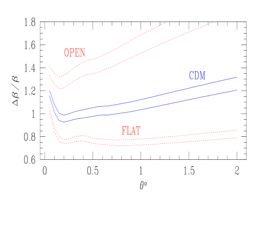
Figure 6: Relative error in $\beta$ for three different underlying cosmological models as a function of the size of the ring $\theta$. The two curves in each case are for beam size $0.22^{o}$ on the top and $0.2^{o}$ on the bottom.

As we are only estimating one parameter the Fisher matrix is just a number ($F$),

$$F={1\over 2}\sum_{k}{\alpha_{k}^{2}\over(\beta\alpha_{k}+w_{P}^{-1})^{2}}.$$ (26)

We can use this Fisher “matrix” to obtain the expected error bars on $\beta$,

$${\Delta\beta\over\beta} = {1\over\beta\sqrt{F}}$$ (27)

$$= \sqrt{2\over\sum_{k}1/(1+w^{-1}_{P}/\beta\alpha_{k})}.$$

This can be interpreted as saying that the effective number of modes contributing informations is $N_{eff}=\sum_{k}1/(1+w^{-1}_{P}/\beta\alpha_{k})$, where clearly the modes with a higher signal to noise contribute more information ($S/N|_{k}=\beta\alpha_{k}/w^{-1}_{P}$).

We can use equation (27) to investigate the effect of changing the size of the ring $\theta$, which enters which enters in the calculation of $\alpha_{k}$. Figure 6 shows $\Delta\beta/\beta$ as a function of $\theta$ for three cosmological models. The $E$ polarization spectra of these models is shown in figure 7, we choose standard CDM (SCDM) and two other models that fit well the available temperature data [15]. One is an open model with $\Omega_{m}=0.85$, $\Omega_{b}h^{2}=0.026$, $h=0.4$ and $n=0.91$. The other is a flat CDM model with $\Omega_{b}=0.05$ and $h=0.3$. It is interesting to note that while this two models have similar temperature spectrum up to the first acoustic peak, within the accuracy of the current CMB measurements, the amplitude of the polarization spectra differ significantly. Figure 6 shows that this experiment may be able to detect polarization in the foreseeable future, at least for some cosmological models. Increasing the sensitivity by reducing the noise and the angular resolution, thus going after the larger small scale polarization, will increase the prospects of the experiment as well.

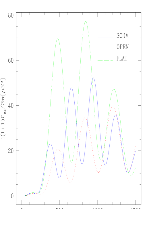
Figure 7: $E$ polarization power spectra for the three models discussed in the text.

The quadratic estimator for beta also takes a very simple form,

$$\hat{\beta}={\sum_{k}(|{\bf x}_{k}|^{2}-w_{P}^{-1})\alpha_{k}/(\beta\alpha_{k}+w_{P}^{-1})^{2}\over\sum_{k}\alpha_{k}^{2}/(\beta\alpha_{k}+w_{P}^{-1})^{2}},$$ (28)

which is nothing more than an inverse variance weighing of each mode. It is straight forward to check that the ensemble average of $\hat{\beta}$ is actually $\beta$ ($\langle|{\bf x}_{k}|^{2}\rangle=\beta\alpha_{k}+w_{P}^{-1}$), it is an unbiased estimator.

In this very simple example we can understand what happens if we construct the estimator using the “wrong” power spectra. Let us assume that the underlying model is SCDM model (ie. that the underlying $\beta=1$ so that $\langle|{\bf x}_{k}|^{2}\rangle=\alpha_{k}+w_{P}^{-1}$) but that we use a different $\beta$ to construct the estimator. The first thing that is easy to check is that $\langle{\hat{\beta}}\rangle=1$ always, the estimator is always unbiased even if we use the incorrect $\beta$ to construct it. What happens is that the variance of the estimator increases if use the incorrect fiducial model, the variance in the estimator is given by

$$\langle{\hat{\beta}}^{2}\rangle-\langle{\hat{\beta}}\rangle^{2}=2{\sum_{k}\alpha_{k}^{2}/(\beta\alpha_{k}+w_{P}^{-1})^{2}\times(\alpha_{k}+w_{P}^{-1})^{2}/(\beta\alpha_{k}+w_{P}^{-1})^{2}\over[\sum_{k}\alpha_{k}^{2}/(\beta\alpha_{k}+w_{P}^{-1})^{2}]^{2}}$$ (29)

This function is shown in figure 8, the variance has a minimum at $\beta=1$. If one chooses an incorrect value of $\beta$ the estimator is still unbiased but is not optimal, one could get more information out of the data (ie. reduce the error bars on $\beta$). Note that the if $\beta\sim 2$ which means we are overestimating the power in the underlying model by a factor of 2, the variance only increases by a few percent. Even for $\beta\sim 4$ the increase is less than 10 %. The curves in figure 8 depend on the signal to noise ratio of the experiment, for example the open model curve grows more slowly than the other two. This model has less power so more of the variance in the estimator comes from the detector noise and so it is less sensitive to the fiducial model.

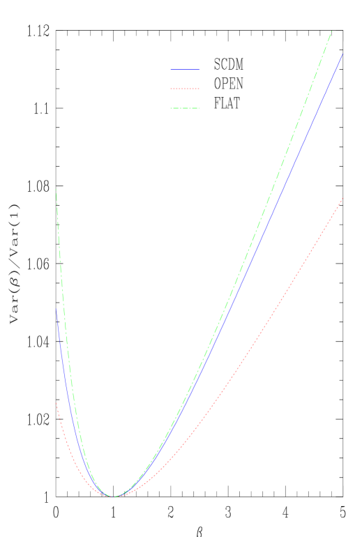
Figure 8: Variance of the ${\hat{\beta}}$ estimator if the underlying model has $\beta=1$ but a fiducial model with a different $\beta$ is used to construct the quadratic estimator. The curves have been scaled using the minimum variance value, when the $\beta=1$ model is used to construct the estimator.

Unfortunately life is not so simple, it is not true that all the models we are interested in testing have a spectrum of the form $C_{El}=\beta{\bar{C}}_{El}$ as is obvious from figure 7. The open and flat models were chosen to fit the existing temperature data [15], this means that their first acoustic peak is approximately in the same place and is approximately of the same height. The acoustic oscillations in the photon-baryon fluid are responsible for both temperature and polarization peaks so if the temperature peaks of two models coincide in position, the polarization ones will also coincide. They not necessarily have the same amplitude, as can be seen in figure 7. To get the best results in this type of analysis we should choose $C_{El}=\beta{\bar{C}}_{El}$ with ${\bar{C}}_{El}$ corresponding to one of the models that fit the existing temperature data. Perhaps polarization can even help distinguish between some of these models before smaller scale temperature measurements do.

In fact if we construct the quadratic estimator under the assumption that the underlying model is the open one, the mean value of $\beta$ if the real model is the flat one is $\langle\beta\rangle=3.033$, figure 9 compares $l(l+1)C_{El}^{flat}/2\pi$ and $\langle\beta\rangle l(l+1)C_{El}^{open}/2\pi$. The agreement is very good especially for the S/N curves for the two models, which is what the experiment is ultimately sensitive to.

In any case $\beta$ should be taken just as an indication of the power in polarization, and because this experiment is sensitive to such a wide range in $l$ it is better to assume some realistic spectrum shape given that the low $l$ polarization is so suppressed. If we do not do so and just assume a flat spectrum the weighing of the $k$ modes in $\hat{\beta}$ will be very bad, leading to an estimator with a very large variance. Of course one could divide the $l$ range in many bins so that the flat approximation in each bin is reasonable, but the S/N in the experiment does not permit that yet. The best way to go is to assume a shape for the spectrum corresponding to some model that fits the existing temperature data well.

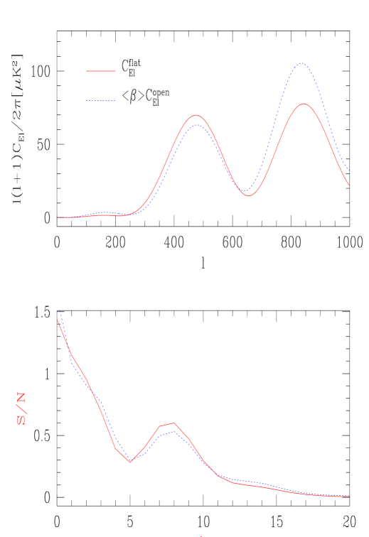
Figure 9: Comparison between the underlying spectrum and the “recovered” one. In the top pannel we show $C^{flat}_{El}$ and $\langle\beta\rangle C_{El}^{open}$. The bottom pannel shows the S/N for each $k$ mode for the flat model and the scaled open one.

4.2 Wisconsin Experiment

Let us now consider the Wisconsin experiment, with the assumption that both $E$ and $B$ spectra are constant, the correlation matrix for each $k$ is

$$\bf{C}_{k} = \langle{\bf x}_{k}{\bf x}_{k}^{{\dagger}}\rangle$$

$$= {\bf E}_{k}\sigma_{E}^{2}+{\bf B}_{k}\sigma_{B}^{2}+w_{P}^{-1}{\bf 1}$$

$${\bf E}_{k} = \left(\begin{array}[]{cc}\alpha_{k,1}&\alpha_{k,3}\\ \alpha_{k,3}&\alpha_{k,2}\end{array}\right)$$ (32)

$${\bf B}_{k} = \left(\begin{array}[]{cc}\alpha_{k,2}&\alpha_{k,3}\\ \alpha_{k,3}&\alpha_{k,1}\end{array}\right),$$ (35)

where $\alpha_{k,j}=\sum_{l\geq k}(2l+1)/4\pi W_{j,lk}$ for $j=1,2$ or $3$ and ${\bf 1}$ is the identity matrix.

Note that there is a symmetry between $(E,B)$ and $(Q,U)$, that is to say interchanging $E$ and $B$ and $Q$ and $U$ leaves equation (35) unchanged. Consider for example the previous signal to noise plot for a model with $\sigma_{E}^{2}=2\mu K^{2}$ and no $B$ (figure 5). In the “conjugate” model having $\sigma_{B}^{2}=2\mu K^{2}$ and no $E$, the $Q$ and $U$ signal to noise plots would just be interchanged. The signal to noise plots for both parameters are different so at least in principle the $E$ and $B$ contributions can be separated.

Figure 10: Contour plots of the $\sigma_{(E,B)}^{2}$ error bars that could be obtained by the Wisconsin experiment for a grid of underlying models with $E$ and $B$ amplitudes between $0\mu K^{2}$ and $10\mu K^{2}$.

We have two parameters so the Fisher matrix is $2\times 2$. we used it to compute the expected error bars on $\sigma_{E}^{2}$ and $\sigma_{B}^{2}$ in a grid of underlying models. Contour plots of the error bars are shown in figure 10. One interesting feature of these plots is that because of the symmetry discussed above both figures are essentially the same, one can go from one to the other by simply interchanging the axis.

The other feature that deserves attention is that for a fixed value of one of the amplitudes, for example $\sigma_{E}^{2}$ as one increases the other one ($\sigma_{B}^{2}$) the error bar on $\sigma_{E}^{2}$ grows. What happens is that the determination of both amplitudes is highly correlated, and always the combination that is better constrained tends to be more aligned with the variable with the highest amplitude. We show the error ellipses in the $\sigma_{E}^{2}-\sigma_{B}^{2}$ plane for two models in figure 11. The first model has $\sigma_{E}^{2}=2\mu K^{2}$ and $\sigma_{B}^{2}=2\mu K^{2}$, the second one $\sigma_{E}^{2}=3\mu K^{2}$ and $\sigma_{E}^{2}=1\mu K^{2}$. Clearly because of the $E-B$ symmetry in the correlation matrix if the underlying model has $\sigma_{E}^{2}=\sigma_{B}^{2}$ the sum of both amplitudes (ie. the total power) is much better constrained than their difference. When we consider a model with more power in the $E$ channel the ellipses rotate so that $\sigma_{E}^{2}$ is better constrained than $\sigma_{B}^{2}$.

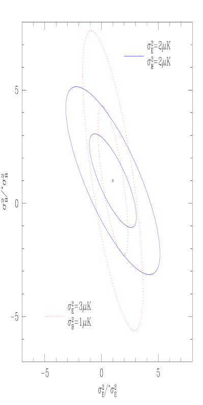
Figure 11: Contour plots of $68\%$ and $95\%$ confidence in the $\sigma_{E}^{2}-\sigma_{B}^{2}$ plane that could be obtained with the Wisconsin experiment. The axis have been scaled using the amplitudes of the underlying models. Two different models are considered.

In figure 12 we show the error bars expected for $\sigma_{E}^{2}$ under the assumption that $\sigma_{B}^{2}=0$, that is models that lay on the x-axis of figure 10. We show two curves, one correspond to trying to determine both $\sigma_{E}^{2}$ and $\sigma_{B}^{2}$ and the other assumes we know there is no $B$ polarization. This is actually a good approximation for most models, only defect models that usually have a large vector contribution have a large $B$ contribution. These models do not seem to be in very good accord with the existing CMB and LSS data [16].

This experiment would be able to detect the cosmological polarization in an underlying model with $\sigma_{E}^{2}\sim 1\mu K^{2}$. A model with $\tau_{ri}=1$ could be detected, but this model has most of its large angular scale power outside the band where the experiment is most sensitive. The “reionization peak” in this case occurs at $l_{peak}\sim 20$ with an amplitude $6\mu K^{2}$, thus a smaller beam would greatly increase the sensitivity of the experiment to the reionization history of the universe, making the experiment better “tunned” for the position of the peak in $l$ space.

It is also clear that a ring experiment can put independent constraints on both $E$ and $B$ separately if it measures $Q$ and $U$. Although the assumption that the spectrum is flat across all the band is not very good in this case, if the noise in the experiment was reduced then several bins in $l$ could be used and our analysis would become more realistic.

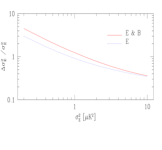
Figure 12: Expected error bars on $\sigma_{E}^{2}$ for models with no $B$ as a function of the underlying models $\sigma_{E}^{2}$. The lower curve results if we assume there is no $B$ rather than fitting for its amplitude.

5 Summary and Discussion

We have studied in detail polarization experiments that measure the Stokes parameters on a ring in the sky. We have shown that the Fourier transform of the Stokes parameters on the ring provides natural variables to analyze the results of the experiment, and have studied how the correlation matrix of this quantities depend on the $E$ and $B$ power spectra. We calculated the window functions and discussed how it depends on the size of the ring.

Experiments that measure both Stokes parameters are capable of determining separately the contributions from both $E$ and $B$. They can do so without assuming a specific shape for each of the spectra because $E$ and $B$ contribute differently to $Q$ and $U$ autocorrelations. In fact for $k=0$ the $Q$ mode only depends on $E$ while the $U$ mode is only sensitive to $B$.

We have calculated the Fisher matrices for these experiments and used them to estimate their ability to detect the amplitude of cosmological polarization. We also constructed the minimum variance quadratic estimator for the parameters of interest and studied their properties in detail

An experiment targeted at small scale polarization measuring the Stokes parameters in a small ring with a fraction of a degree resolution, may detect cosmological polarization in the near future. In fact, with sufficient integration it may help distinguish between models that have very similar temperature power spectra in the $l$ range measured so far and so could add useful information.

The Wisconsin experiment is mostly sensitive to large scale polarization but because the signal in this part of the spectrum is very small it will be harder for it to detect polarization. On the other hand the measurement of both $Q$ and $U$ will allow the experiment to put separate constraints on $E$ and $B$.

The prospect of detecting polarization is increasing quickly and in the near future we may have a positive detection. We will then be able to study very interesting characteristics of our universe, like its ionization history or the presence of vector and tensor modes.

6 Appendix

In this appendix we will consider the window functions for the Wisconsin Experiment. This experiment will be pointing in the vertical direction scanning a ring in the sky with $\theta=43^{o}$. The instrument will be rotated in steps of $45^{o}$ to measure both $Q$ and $U$ . The signal at each pixel is given by

$$X_{j}={1\over\delta t}\int_{t_{o}-\delta t/2}^{t_{o}+\delta t/2}dt\int d\Omega^{\prime}B({\hat{n}}(t),{\hat{n}}^{\prime})X(\hat{n})$$ (36)

where $X$ stands for the Stokes parameter being measured, $j$ represents the pixel and $\delta t$ is the time interval the instrument is measuring each particular Stokes parameter before being rotate by $45^{o}$ degrees. The beam is represented by the convolution with $B(({\hat{n}}(t),{\hat{n}}^{\prime})$ and ${\hat{n}}(t)$ is the instantaneous position of the beam, in this case given by $\theta=43^{o}$ and $\phi=\omega_{s}t$ with $\omega_{s}=2\pi/$day.

We can use the expansion in harmonics (equation 4) to calculate the convolution with the beam. For a gaussian beam this gives the usual factor $\exp{[-l(l+1)\sigma_{b}^{2}/2]}$. For example

$$Q_{j} = {1\over\delta t}\int dt[-\sum_{lm}a_{E,lm}e^{-l(l+1)\sigma_{b}^{2}/2}X_{1,lm}(\theta,\phi(t))$$ (37)

$$+ia_{B,lm}e^{-l(l+1)\sigma_{b}^{2}/2}X_{2,lm}(\theta,\phi(t))]$$

and a similar expression applies to $U$.

The time integration is simple, the dependence is only in the $\exp{[im\phi(t)]}$ factors inside $X_{(1,2),lm}$. The window function then acquires another factor from

$${1\over\delta t}\int dte^{im\phi(t)}=e^{im\phi_{j}}{\sin(m\Delta\phi/2)\over m\Delta\phi/2}$$ (38)

with $\Delta\phi=\omega_{s}\delta t$, the size of the pixel. The combined window is $B_{lm}=\exp{[-l(l+1)\sigma_{b}^{2}/2]}{\sin(m\Delta\phi/2)/(m\Delta\phi/2)}$. The importance of this last term depends on the size of the pixel, and can be made irrelevant by choosing small enough pixels. We ignored this factor in the main text for simplicity, but it can trivially be accounted for.

References

• [1] M. Zaldarriaga, D. N. Spergel and U. Seljak, Report no. astro-ph/9702157, 1997 (ApJ in press).
• [2] D.N. Spergel, 1994 Warner Prize Lecture, Bull. Amer. Astron. Soc., 26, 1427 (1994); G. Jungman et al.. M. Kamionkowski, A. Kosowsky, and D. N. Spergel, Phys. Rev. Lett. 76, 1007 (1996); ibid Phys. Rev. D 54 1332 (1996); J.R. Bond, G. Efstathiou & M. Tegmark, Report no. astro-ph/9702100
• [3] M. Zaldarriaga, Phys. Rev. D 55 1822 (1997).
• [4] M. Zaldarriaga and U. Seljak, Phys. Rev. D 55 1830 (1997); U. Seljak and M. Zaldarriaga Phys. Rev. Lett. 78, 2054 (1997).
• [5] M. Kamionkowski et al., Report no. astro-ph/9609132, ibid astro-ph/9611125, 1996 (unpublished)
• [6] D. Spergel and M. Zaldarriaga, Report no. astro-ph/9705182 (Phys. Rev. Lett. in press)
• [7] U. Seljak, U. Pen and N. Turok, Report no. astro-ph/9704231 (unpublished)
• [8] Keating, B., Timbie, P., Polnarev, A., and Steinberger, J., accepted for publication in ApJ
• [9] Chandrasekhar, S. 1960, in Radiative Transfer (Dover: New York)
• [10] Goldberg, J. N., et al. 1967, J. Math. Phys. 8, 2155
• [11] W. Hu and M. White, Report no. astro-ph/9706147 (New Astronomy in press)
• [12] U. Seljak, Ap. J. 482 6
• [13] M. Tegmark, Andy Taylor and Alan Heavens Ap. J. 480 (1997) 22-35
• [14] J. R. Bond, A. H. Jaffe and L. Knox Report no. astro-ph/9708203 (unpublished)
• [15] C. H. Lineweaver, D. Barbosa, A. Blanchard and J. G. Bartlett Report no. astro-ph/9610133 (Astro. & Astrophysics in press); C. H. Lineweaver and D. Barbosa Report no. astro-ph/9706077 (unpublished)
• [16] U. Pen, U. Seljak and N. Turok, Report no.astro-ph/9704165 (unpublished)