Metal enrichment of the intergalactic medium

Abstract

I demonstrate by means of high resolution cosmological simulations, which include modelling of a two-phase interstellar medium, that the dominant mechanism for transporting heavy elements from the proto-galaxies into the IGM is the merger mechanism as discovered by Gnedin & Ostriker. Direct ejection of the interstellar gas by supernovae plays only a minor role in transporting metals into the IGM: for a realistic cosmological scenario only a small fraction of all metals in the IGM is delivered by the supernova-driven winds, while most of all metals in the IGM are transported by the merger mechanism. As the result, the metallicity distribution in the IGM is highly inhomogeneous, in agreement with studies of the QSO metal absorption systems, and the predicted metallicity distribution of Lyman-alpha absorbers as a function of their column density is in excellent agreement with the observational data.

1 Introduction

It is now well established that the Lyman-alpha forest absorbers, thought to mostly consist of density peaks in the low density intergalactic medium away from (proto-)galaxies (Cen et al. 1994; Zhang et al. 1995; Petitjean, Mucket, & Kates 1995; Hernquist et al. 1996; Miralda-Escudé et al. 1996; Wadsley & Bond 1996; Bi & Davidsen 1996; Hui, Gnedin, & Zhang 1996), contain a measurable, about 1% of solar, amount of heavy elements (“metals”) at a redshift as high as three and even beyond. An early indication to this extent by Meyer & York (1987) is now confirmed quantitatively by new high-resolution Keck data (Womble, Sargent, & Lyons 1995; Songaila & Cowie 1996), who found that as a column density of the Lyman-alpha absorbers decreases, smaller and smaller fraction of all absorbers contain a measurable amount of heavy elements, indicating highly inhomogeneous distribution of metallicities in the intergalactic medium (IGM). What is the origin of those metals and their inhomogeneous distribution?

Within the boundaries of standard astrophysics, there is only one “factory” that produces metals - stars. Stars lose mass via winds and explode as supernovae, polluting the interstellar medium with metals. However, from a cosmological point of view, there is a long way from the interstellar medium, which has a cosmological overdensity $\delta$ ($\delta\equiv\rho/\bar{\rho}-1$) of about $10^{4}\div 10^{5}$, to the intergalactic medium with overdensities of about $10$ and below; any mechanism that transports metals from the proto-galaxies into the IGM should therefore be powerful enough to overcome the gravitational force associated with enormous overdensities of (proto-)galaxies.

For a long time since the pioneering works by Couchman & Rees (1986) and Dekel & Silk (1986; see also Miralda-Escudé & Rees 1997 for a recent review) it has been thought that the supernovae blowing out gas from the Population III objects would do the job. However, recent numerical three-dimensional simulations (Ostriker & Gnedin 1996; Gnedin & Ostriker 1996) as well as semi-analytical results (Haiman, Rees, & Loeb 1996) convincingly demonstrated that Pop III objects, formed via molecular hydrogen cooling, are so few (mostly because the molecular hydrogen is so fragile), that they are unable to produce the metallicity in excess of about $10^{-5}$ solar.

Nevertheless, supernovae can still disrupt normal, Pop II, proto-galaxies and pollute the IGM with metals, as argued, for example, by Miralda-Escudé & Rees (1997). If it were the only mechanism for transporting metals from the deep potential wells of proto-galaxies into the diffuse IGM, it would be the final answer to the question: “What is the metal transport mechanism in the IGM?”. However, as was discovered by Gnedin & Ostriker (1996), there exists another metal transport mechanism, which is based solely on gravitational hierarchical clustering. Namely, when two proto-galaxies merge with a sufficiently large relative velocity in a close to head-on collision, dark matter halos and stellar components of two halos penetrate through each other, whereas gas components of both objects collide in a gigantic shock. The pressure force arising from this interaction is comparable to the gravitation force from the dark matter and baryons of two objects. Therefore, the collisionless component (the dark matter and stars) and the collisional component (the interstellar gas) experience forces that significantly differ in their directions and amplitudes, and, as the result, both components may have different spatial distributions in the process of merging. Because the gas constitutes only a small fraction of the total mass of a proto-galaxy, it often happens during those violent mergers that some fraction of the gas (typically a few percent), displaced relative to the dark matter, becomes gravitationally unbound and gets ejected from the proto-galaxy into the IGM. This gas, which was a part of the interstellar medium in the past, and is heavily enriched with metals, gets mixed up with the surrounding IGM, polluting it with heavy elements. As the result, the metal distribution in the IGM becomes highly inhomogeneous: while regions around the proto-galaxies are enriched with heavy elements, the centers of large voids, well removed from the places where merging occurs, still contain the pristine material (an example of how this mechanism works is shown in Gnedin & Ostriker 1996 and will not be presented in this paper).

One can imagine other ways to transport metals from the proto-galaxies to the IGM. For example, a fraction of young stars can be lost during a merger, and going off later as supernovae, may enrich the IGM. I consider this process a part of merging mechanism, and will not distinguish it from the case when the metal enriched gas rather than stars was lost in the merger. After all, since stars are subject to the same (purely gravitational) force as the dark matter is, and the gas is not, it is much easier to unbound a substantial fraction of the total gas component of two merging proto-galaxies rather than of their stellar component.

The whole process of the metal enrichment of the IGM begins in stars: stars make metals in the first place in the gas with the cosmic overdensity of $\delta\sim 10^{30}$; blowing up as supernovae, they enrich the ISM ($\delta\sim 10^{5}$) with metals; metals from the ISM get transported into the IGM ($\delta\mathrel{\mathchoice{\vbox{\offinterlineskip\halign{\hfil$\reset@font\displaystyle#$\hfil\cr<\cr\sim\cr}}}{\vbox{\offinterlineskip\halign{\hfil$\reset@font\textstyle#$\hfil\cr<\cr\sim\cr}}}{\vbox{\offinterlineskip\halign{\hfil$\reset@font\scriptstyle#$\hfil\cr<\cr\sim\cr}}}{\vbox{\offinterlineskip\halign{\hfil$\reset@font\scriptscriptstyle#$\hfil\cr<\cr\sim\cr}}}}10$) either by the very same supernovae or by the merging mechanism as explained above. It is therefore the purpose of this paper to investigate the relative importance of those two metal transport mechanisms within the framework of a reasonable cosmological model.

Since the transition between the ISM and the IGM is somewhat uncertain, and in order to avoid introducing another, “intermediate”, component for the cosmic gas, I will call “the ISM” the gas that is gravitationally bound to a particular proto-galaxy, and “the IGM” the rest of the cosmic gas (i.e. gas, which is not bound to a particular self-gravitating object).

Several attempts have been made before to include effects of supernovae into cosmological hydrodynamic simulations (c.f. Cen & Ostriker 1992; Navarro & White 1993; Katz, Weinberg, & Hernquist 1996). However, all previous works attempted to model the ISM as a single-phase medium, simply injecting thermal and kinetic energy of supernovae into the cosmic gas. This approach is strongly dependent on the numerical resolution of a simulation. For a low resolution simulation, injection of thermal energy may produce a significant effect. However, as the resolution of a simulation increases, and higher and higher density regions are being resolved, the cooling time in the gas becomes smaller and smaller, and any amount of the thermal energy that is directly injected into the cosmic gas, is radiated away before it has had a change to influence the dynamics of the gas. In reality however, the thermal energy gets injected in supernova remnant bubbles (the second phase in the gas), that are too hot and do not cool as efficiently.

On the other hand, the kinetic energy directly injected into the gas can propagate a large distance from the source of injection, because the unsufficient resolution of a simulation prevents one to resolve the snow-plow phase of the supernova remnant evolution (Cioffi, McKee, & Bertschinger 1988; McKee 1990), during which most of the kinetic energy of the supernova ejecta is absorbed. Thus, the effect of the finite numerical resolution can lead to both underestimating and overestimating the effect of the supernovae on the dynamics of the ISM, depending on the resolution of a simulation and details of the implementation of the supernova feedback. Because the resolution of a high-resolution Lagrangian simulation is not uniform across the simulation volume, and varies from point to point, it is extremely difficult to disentangle the physical effect of supernovae feedback from numerical artifacts produced by the finite resolution of a simulation.

It is therefore logical to attempt to model the multi-phase ISM in order to account properly for the supernovae feedback. Again, the finite resolution of existing cosmological hydrodynamic simulations does not allow to resolve properly the evolution of a single supernova remnant, but the multi-phase ISM can be incorporated in a cosmological simulation as “sub-cell” physics, similar to the way the star formation is included in simulations. In other words, for a sufficiently large region, which contains many supernovae, it is possible to account for the total effect, a population of supernova remnants have (on average) on the dynamics of the interstellar gas (energy injection, extra pressure, reduction in the star formation rate etc).

Simulations reported on in this paper attempt to do precisely that. The main difference between this work and previous investigations is that a two-phase medium is now allowed for in a simulation, i.e. at each point in a simulation the cosmic gas has two temperatures (the “cold” phase outside the supernova remnants and “hot” phase inside the supernova remnants) and two densities (which can be expressed as the total density and the volume fraction occupied by the hot phase). The current implementation explicitly assumes however that the population of supernova remnants is moving together with the rest of the cosmic gas, i.e. the two phases have the same velocity on a large ($\sim 1\mbox{\,kpc}$) scale. The velocity itself is however affected by the feedback from the supernova remnants. The specific recipe for incorporating physics of the two-phase ISM into a cosmological hydrodynamic code is presented in Appendix A.

Finally, a few words about interpreting results of a cosmological simulation. Any “sub-cell”, phenomenological description of a physical process like supernova feedback or star formation inevitably introduces new parameters that describe the physical process under consideration. It is currently unrealistic (from the point of view of computational resources) to perform a full-scale extensive parameter study, and thus it should be kept in mind that any cosmological hydrodynamic simulation which includes “sub-cell” physics (including simulations reported on in this paper) should be considered as a plausible possibility rather than the final answer. There always remains a chance that the nature picked up different values of parameters than those used in a simulation, however plausible the latter seem to be.

2 Method

I have adopted a CDM+$\Lambda$ cosmological model as a framework for these investigations. The qualitative results of my simulation are applicable to the whole family of the CDM-type models, and I emphasize those qualitative conclusions together with specific quantitative results for the model I use. The cosmological parameters are fixed as follows:

$$\begin{array}[]{rcl}\Omega_{0}&=&0.35,\\ \Omega_{\Lambda}&=&0.65,\\ h&=&0.70,\\ \Omega_{b}&=&0.055,\\ \end{array}$$

which is one of the cosmological models adopted by the Grand Challenge Cosmological Consortium (GC³) as the “best-bet” models (http://arcturus.mit.edu/GC3/IC). This model is similar to the model investigated by Gnedin & Ostriker (1996) except that $\Omega_{b}$ has a higher value, in concordance with the low primordial abundance as inferred by Tytler & Burles (1996).

Since the merging mechanism can only be studied by a numerical simulation, I use the SLH-P³M cosmological hydrodynamic code as described by Gnedin (1995), Gnedin (1996), Gnedin & Bertschinger (1996), and Gnedin & Ostriker (1996). However, since the goal of this paper is to study the effects of supernovae on the metal transport in the IGM, a proper numerical treatment of the physical effect of supernovae has to be incorporated in the code. Appendix A explains how the physics of the multi-phase interstellar medium can be incorporated into a cosmological hydrodynamic code on scales large compared to the size of one supernova bubble. Three parameters control the evolution of the ISM in this regime: $E_{51}$, the average energy of a supernova measured in units of $10^{51}\mbox{\,erg}$, $f_{\rm IMF}$, a factor parametrizing the excess (lack) of metal production compared to the Miller-Scalo IMF, and $v_{\rm term}$, the termination velocity of the supernova shock at which the interior of the bubble is ionized. In order to minimally span the parameter space and understand how supernovae effect the IGM on different scales, six simulations have been performed. Each simulation has $64^{3}$ dark matter particles, $64^{3}$ gas cells, and a number of stellar particles which are being formed during a simulation. The softening parameter for all simulations is set to $1/10$, corresponding to the dynamical range of $640$. In addition to the new ingredient, the physics of the supernova, physical modelling in all runs includes all components described in Gnedin (1996) and Gnedin & Ostriker (1996), to which papers the reader is referred for more details about physical modelling. Here I only note that I allow for the fully three-dimensional treatment for the evolution of the dark matter and the two-phase cosmic gas, as well as for the formation and destruction of molecular hydrogen and all other standard physical processes for a gas of primeval composition, following in detail the ionization and recombination of all species in the ambient radiation field. The spatially and frequency dependent radiation field, in turn, allows for sources of radiation (quasars and massive stars), sinks (due to continuum opacities), self-shielding of the dense gas lumps, and cosmological effects. In regions which are cooling and collapsing (beyond the numerical resolution of the code) I allow the formation of point-like “stellar” subunits, permitting them to release radiation and explode as supernovae. Supernovae inject thermal and kinetic energy in the ISM (via the second gaseous phase - the supernova remnants), and pollute the surrounding gas with metals, which are in turn considered in the treatment of cooling.

Parameters of all runs are summarized in Table 2.

Table 2: Numerical Parameters

Run	Box size	Spatial res.	$E_{51}$	$f_{\rm IMF}$	$v_{\rm term}$
A1	$1h^{-1}{\rm\,Mpc}$	$1.6h^{-1}{\rm\,kpc}$	0	4	NA
B1	$1h^{-1}{\rm\,Mpc}$	$1.6h^{-1}{\rm\,kpc}$	1	4	$c_{S}$
C1	$1h^{-1}{\rm\,Mpc}$	$1.6h^{-1}{\rm\,kpc}$	1	4	$30\mbox{\,km}/\mbox{\,s}$
A3	$3h^{-1}{\rm\,Mpc}$	$4.7h^{-1}{\rm\,kpc}$	0	4	NA
B3	$3h^{-1}{\rm\,Mpc}$	$4.7h^{-1}{\rm\,kpc}$	1	4	$c_{S}$
C3	$3h^{-1}{\rm\,Mpc}$	$4.7h^{-1}{\rm\,kpc}$	1	4	$30\mbox{\,km}/\mbox{\,s}$

In order to span a large enough range in mass scales, two sets of runs are performed: the first set with the $1h^{-1}\mbox{\,Mpc}$ box size and the total mass resolution of $10^{5.6}h^{-1}{\rm M}_{\odot}$, and the second set with the $3h^{-1}\mbox{\,Mpc}$ box size and the total mass resolution of $10^{7.0}h^{-1}{\rm M}_{\odot}$. The resolution in baryons is a factor of $0.055/0.35=0.16$ finer, and for runs with the $1h^{-1}\mbox{\,Mpc}$ box size, it is $10^{4.8}h^{-1}{\rm M}_{\odot}$, which is about the Jeans mass at $z\sim 15$ for this model. Those runs, therefore, account for all initial fluctuations that are present in the baryons, i.e. they do not miss any small scale power in the initial conditions (but those simulations do miss the small scale power that is generated by the nonlinear dynamics at later times on the scales below the resolution limit).

Simulations within each set have had exactly the same initial conditions; so that evolution of individual objects can be followed under different physical assumptions. Because it makes no sense to continue a simulation of a finite size beyond the redshift when perturbations with the wavelength of the order of the box size become nonlinear, runs with $3h^{-1}\mbox{\,Mpc}$ box size are stopped at the redshift $z=4$, and runs with $1h^{-1}\mbox{\,Mpc}$ box size are not continued beyond $z=9$.

In each of two sets three different runs have been performed:

run A,

when no physics of the multiphase ISM (as described in Appendix A) has been taken into account (manifested by the parameter $E_{51}$ set to zero); this run does not include effects of supernovae, and therefore only the merging mechanism for metal transport operates in this case; this run is then used for comparison with two other runs where effects of supernovae are included, to assess the relative importance of two metal transport mechanisms.

run B,

which includes physics of the multiphase ISM; in this run it is assumed that the supernova shock is terminated at the sound speed of the ambient medium.

run C,

which includes physics of the multiphase ISM; in this run the supernova shock is terminated at the velocity of $30\mbox{\,km}/\mbox{\,s}$.

The latter choice is somewhat arbitrary; it approximately maximizes the effect of supernova on heating of the low metallicity ISM. As has been shown by Shull & McKee (1979), the supernova shock in the ISM with solar metallicity fails to ionize the gas at shock velocities below $90\mbox{\,km}/\mbox{\,s}$. It is expected that for low metallicity gas at high redshift this value is somewhat lower (Shull & Silk 1981), and I somewhat arbitrary fix it to be $30\mbox{\,km}/\mbox{\,s}$, near the value which maximizes the effect of supernovae. This choice also allows for the possibility that the star formation occurs inside the dense supernova swept-up shells, which are considered belonging to the cold phase for the shock velocities below $30\mbox{\,km}/\mbox{\,s}$.

Finally, I choose a factor $f_{\rm IMF}=4$, which implies that I assume a top-heavy IMF, with a factor of four higher metal production then in the solar neighborhood. As argued by Silk (1996), this value is supported by metal abundances in the clusters of galaxies if one assumes that all metals came from cluster galaxies alone. This number is an extreme, in a sense that if the clusters of galaxies contain additional stars which are distributed over the cluster (and which would be virtually unobservable), then $f_{\rm IMF}$ should be less than 4. Both runs C1 and C3 should therefore be considered as limiting cases when all possible parameters are pushed to their extreme values in order to maximize the effect of supernovae.

3 Results

3.1 The Metallicity of the IGM

Figure 2: Upper panel: the comoving star formation rate in units of $\mbox{\,M}_{\odot}/\mbox{\,yr}/(h^{-1}\mbox{\,Mpc})^{3}$ as a function of redshift for six runs: A1 (thin solid line), B1 (thin dotted line), C1 (thin dashed line), A3 (bold solid line), B3 (bold dotted line), and C3 (bold dashed line). Lower panel: the mass weighted mean metallicity of the cosmic gas as a function of redshift; line markings are as on the upper panel.

As the cosmic structure develops under the influence of gravity, baryons condense into bound objects, cool and eventually form stars, which end their lives as supernovae and pollute the environment (i.e. ISM and IGM) with metals. Figure 2 shows in the upper panel the comoving star formation rate in units of $\mbox{\,M}_{\odot}/\mbox{\,yr}/(h^{-1}\mbox{\,Mpc})^{3}$ for all six runs: the bold lines indicate runs A3-C3, and the thin lines correspond to runs A1-C1. The solid lines mark runs A, the dotted lines mark runs B, and the dashed lines mark runs C. In all figures below line markings are the same unless specified otherwise. Note that the star formation declines at late epochs due to the final size of a simulation box (and, as the result, lack of large-scale power to drive the gravitational collapse further).

The lower panel of the same figure shows the mass-weighted average metallicity of the cosmic gas (i.e. ISM and IGM together) as a function of redshift. I would like to note here, that simulations with different box sizes are reasonably consistent with each other in a sense that runs with the $3h^{-1}\mbox{\,Mpc}$ box size (A3-C3) have similar star formation rates and metallicities at $z=9$, when runs with the $1h^{-1}\mbox{\,Mpc}$ box size (A1-C1) become unreliable because of the missing large-scale power.

As can be seen, both the star formation rates and the average metallicities for runs with the $1h^{-1}\mbox{\,Mpc}$ box size are somewhat suppressed in cases when supernova effects were taken into account (runs B1 and C1, thin dotted and dashed lines) as compared to the case when no supernova effects were included (run A1, the thin solid line). It is the expected result, since as the volume fraction occupied by supernova bubbles increases, a smaller and smaller fraction of the gas is available for star formation, because the gas inside the bubbles is hot and is not able to cool fast enough. However, even on the smallest resolved scales this effect is not dramatic: in the most favored case (C1) both the star formation rate and the average metallicity are decreased by $z=9$ by a factor of 2.5, but not by orders of magnitude.

Figure 4: The mass- (upper panel) and volume- (lower panel) weighted probability distribution to find a fluid element with given values of the metallicity and the cosmic gas density for run A3 at $z=4$. The bold line shows the contour corresponding to the probability $P(Z=\langle Z\rangle,\delta=0)/4$, solid contours mark the probability higher and the dashed contours show the probability lower than the one marked with the bold contour; contour spacing is logarithmic with the increment of $1/3$ dex.

Before I proceed further with more detailed comparison between the two main mechanisms of metal transport in the IGM, it is instructive to discuss the spatial distribution of the metallicity. Figure 4 shows the mass- (the upper panel) and the volume-weighted (the lower panel) probability distributions for a fluid element to have given values of the metallicity and the gas density (as measured by the overdensity $\delta=\rho/\bar{\rho}-1$) from run A1 at $z=4$ (a similar figure is presented in Gnedin & Ostriker 1996). The immediate conclusion is that the distribution is quite broad, with regions at about the cosmic mean density having values of metallicity all the way from zero to about solar (at $z=4$ !). The distribution narrows down in the high density limit, because the high density gas resides inside the proto-galaxies and is enriched with metals. This high-density, metal-rich gas occupies only a small fraction of the volume, so, if there is a substantial fraction of the gas with metallicities as high as tenth of solar (at $z=4$ !), most of the volume is occupied by the low metallicity gas. This wide distribution of metallicities is in agreement (at least qualitatively) with the recent conclusions by Rauch, Haehnelt, & Steinmetz (1996) and by Hellsten et al. (1997), who found that the observed scatter in the abundance ratios of the QSO metal absorption systems is inconsistent with the assumption of the uniform metallicity. The required scatter in the metallicity at a given value of the cosmic density is about an order of magnitude, which is consistent with Fig. 4 for $\delta\mathrel{\mathchoice{\vbox{\offinterlineskip\halign{\hfil$\reset@font\displaystyle#$\hfil\cr>\cr\sim\cr}}}{\vbox{\offinterlineskip\halign{\hfil$\reset@font\textstyle#$\hfil\cr>\cr\sim\cr}}}{\vbox{\offinterlineskip\halign{\hfil$\reset@font\scriptstyle#$\hfil\cr>\cr\sim\cr}}}{\vbox{\offinterlineskip\halign{\hfil$\reset@font\scriptscriptstyle#$\hfil\cr>\cr\sim\cr}}}}10$.

I emphasize here that Fig. 4 presents the total cosmic gas, including both the ISM and the IGM. The gas with overdensities in excess of $10^{3}\div 10^{4}$ is apparently located inside the proto-galaxies, and is identified with the ISM. The low density gas, $\delta\mathrel{\mathchoice{\vbox{\offinterlineskip\halign{\hfil$\reset@font\displaystyle#$\hfil\cr<\cr\sim\cr}}}{\vbox{\offinterlineskip\halign{\hfil$\reset@font\textstyle#$\hfil\cr<\cr\sim\cr}}}{\vbox{\offinterlineskip\halign{\hfil$\reset@font\scriptstyle#$\hfil\cr<\cr\sim\cr}}}{\vbox{\offinterlineskip\halign{\hfil$\reset@font\scriptscriptstyle#$\hfil\cr<\cr\sim\cr}}}}10$, is clearly a part of the IGM (and is, therefore, partly pristine), with the gas at intermediate densities belonging to the ISM or the IGM, depending on whether it is bound to a particular self-gravitating object or not.

Figure 6: The average metallicity of the gas as a function of the cosmic gas density at $z=4$ (left panel) and $z=9$(right panel). Line markings as in Fig. 2 except for $z=4$ case where no lines for runs A1-C1 are shown since those runs were stopped at a higher redshift.

In order to compare the metallicity-density relationship for different runs, I consider how the average metallicity changes with the gas density. For of all fluid elements having the overdensity $\delta$ within the range from $\delta$ to $\delta+d\delta$, I compute their metallicity $Z(\delta)$ as a function of $\delta$ and plot it in Figure 6 in units of the mass-weighted average metallicity for all six runs (in the other words, the solid bold line in the left panel is Fig. 4 collapsed along the vertical direction, and other lines are produced from the metallicity-density distributions for other respective runs; line markings are again as in Fig. 2). The left panel shows runs (A3-C3) at $z=4$ (since runs A1-C1 were stopped at $z=9$), and the right panel shows all six runs at $z=9$.

The fact that all three lines almost coincide in the left panel of Fig. 6 demonstrates that at intermediate redshifts ($z\sim 4$) and large scales ($\sim 100\mbox{\,kpc}\div 1\mbox{\,Mpc}$) supernovae play no role in transporting metals into the IGM. It is the merging mechanism that enriches the IGM with heavy elements and produces a highly inhomogeneous distribution of metallicities. Even at higher redshifts, and on smaller scales, supernovae play a minor role as a metal transport mechanism in the IGM. However, in the right panel of Fig. 6 ($z=9$) one can notice that in run C1 (the most favorable for the supernovae effects) there is a fraction of gas sitting at very low densities (about 0.01 of the mean) and having the metallicity 40 times above the average (about 10% solar). This would be a signature of the supernova ejected gas, which would be highly enriched with metals and would have low densities, since its temperature is higher (about $10^{5}\mbox{\,K}$) that the average temperature of the IGM at this high redshift ($10^{3}\div 10^{4}\mbox{\,K}$). However, except for this very low density gas, differences in the metallicities between runs with supernovae (B,C) and runs without supernovae (A) are not significant for the IGM with the density higher than the cosmic mean.

Figure 8: The mass-weighted probability distribution to find a fluid element with given values of the metallicity and the cosmic gas density for runs A1 (solid lines) and C1 (dashed lines) at $z=9$. The contour spacing is as in Fig. 4. The low-density - high-metallicity region of the plane in run C1 (supernova blown gas) accounts for 0.03% of the total gas mass and 0.6% of the total volume.

The difference between runs A1 (no supernovae) and C1 (most efficient supernovae) is further demonstrated in Figure 8, which shows the mass-weighted metallicity-density distributions for those two runs in a fashion similar to the upper panel of Fig. 4, except that two different line markings now correspond to two runs: the solid lines show contours for runs A1, and the dashed lines show contours for run C1. The two distributions are very similar except for a small amount of the very low density - high metallicity gas which is present in run C1 but is absent in run A1. This gas is blown out of a proto-galaxy by the supernova activity; its amount is insignificant: it occupies 0.6% of the total volume and amounts to 0.03% of the total gas mass in the universe. This gas is not necessarily the only gas that was ejected from the proto-galaxies by supernovae: there are slight differences in the metallicity-density distributions in runs A1 and C1 at higher densities, which are due to differences in the star formation rates and the supernova activity (but those two can not be meaningfully separated). However, in the whole, the supernova mechanism plays a minor role in transporting metals into the IGM, and by $z\sim 4$ gas disruption in violent mergers is responsible for delivering of more than 99% of all heavy elements in the IGM.

One may ask a question: what is fraction of the enriched gas in the colliding high redshift objects which gets unbound and ejected into the IGM? It might not be appropriate to talk about a single value, but it is easy to come up with an upper limit. Let me consider an oversimplified picture of the universe, which consists of high-density bound objects with the average metallicity $Z_{H}$, which contain $f_{H}$ of the total mass. The rest of the universe is in the IGM, with the average metallicity $z_{L}$. I also assume that bound objects occupy a negligible fraction of the volume. In this case, the volume weighted averaged metallicity will be just $Z_{L}$. For the run A3 at $z=4$, this value is $Z_{L}=6\times 10^{-3}Z_{\odot}$. The mass weighted average metallicity in this case is $\langle Z\rangle_{M}=Z_{H}f_{H}+Z_{L}f_{L}$. For run A3 at $z=4$ the respective values are $f_{H}=0.2$ and $\langle Z\rangle_{M}=5\times 10^{-2}Z_{\odot}$, which implies that the average metallicity of bound objects $Z_{H}=0.23Z_{\odot}$. Since all metals in the IGM come from the gas that gets unbound in mergers, the fraction $f_{\rm unb}$ of this gas is

• $\displaystyle\hskip 0.0pt{f_{\rm unb}={Z_{L}f_{L}\over Z_{H}f_{H}+Z_{L}f_{L}}=10\%.}$

This number is however an upper limit, since I have assumed that the bound objects occupy no volume at all, because any clustering in the IGM will decrease this bound as well, and because the limited resolution of my simulations underestimates the mass fraction $f_{H}$ locked in bound objects.

More than ten years ago Dekel & Silk (1986) analysed the effect of supernovae on the gas ejection from high redshift proto-galaxies using the analytical approach. They found that supernovae can efficiently expel gas from low mass proto-galaxies provided that the star formation is extremely rapid and is happening on a free-fall time scale. I point out here that there are two important physical effects, which are included in the simulations presented here, but omitted in the Dekel & Silk (1986) calculations. First, the negative feedback [eq. (A8)] limits the star formation rate when the fraction of the volume occupied by supernova remnants becomes large. This effects is ignored in Dekel & Silk (1986) paper. Second, Dekel & Silk (1986) ignore cooling of the interstellar gas, which leads to a substantial loss of energy injected by the supernova. For example, if all of the supernova energy was simply injected into the ISM gas without proper account for the two-phase ISM and supernova remnant evolution, all energy would be radiated away, producing negligible net effect.

One can therefore ask a question whether the present work conflicts with the conclusions of Dekel & Silk (1986). I would like to emphasize here that this paper does not pretend to claim that the supernovae do not eject gas from bound objects, and as I show in the following section, they sometimes do it very efficiently. Thus, the supernova ejection is a mechanism for metal transport into the IGM. However, as I explained above, there is another metal transport mechanism, the merger mechanism, and the simulations presented in this paper support the conclusion that the merger mechanism is more efficient. The major physical reason for that is that the merger mechanism works irrespectively of the binding energy of an object and of the star formation rate in the object, whereas supernovae are able to disrupt the gas from a bound object only for objects with sufficiently low masses and high star formation rates. More than that, in order to transfer metal enriched gas into the IGM, it is required to expel the gas not just beyond the virial radius of the dark matter halo, but beyond the turn-around radius; otherwise, the expelled gas will fall back into the dark matter halo in a fraction of a Hubble time.

Therefore, it has to be kept in mind that the results presented in this paper do not necessarily contradict the conclusions of Dekel & Silk (1986), but a more careful comparison will have to be performed in order to verify whether the simulations actually confirm the conclusions of Dekel & Silk (1986).

3.2 Supernovae in the Proto-Galaxies

Figure 10: Properties of all bound objects containing more than 100 particles identified at $z=9$ in runs A1 (left column), B1 (middle column), and C1 (right column). Shown in three rows as a function of the total mass of an object are the gas fraction for each object (upper row), the stellar fraction (middle row), and the fraction of the hot gas within the supernova remnants (lower row). The only object whose gas was completely disrupted by the supernova activity in run C1, and the same objects in runs A1 and B1, are marked with a circle in the upper row and in the right column.

As I have demonstrated in the previous section, the supernova-driven winds are less efficient in transporting metals in the IGM than the merger mechanism. Nevertheless, supernova disruption of proto-galaxies does happen, as the difference between runs A1 and C1 is due to the gas disrupted by the supernovae from the proto-galaxies. In order to understand this process, I show in Figure 10 properties of all well-resolved (containing more than 100 particles of all kinds) bound objects identified at $z=9$ in runs A1 (the left column), B1 (the middle column), and C1 (the right column). Three rows show the gas fraction, the stellar fraction, and the fraction of the hot gas within the supernova remnants for each object versus its total mass (the lower left panel is empty because the supernova effects are not included in run A1). The fraction of the hot gas never exceeds about 30% since it is averaged over the whole object, including the outer regions where there is no star formation (and thus the supernova activity); in most of the objects it reaches close to 100% in the center, where star formation takes place. In run C1 fractions of the hot gas are smaller that the respective fractions in run B1, because the supernova remnants are assumed to terminate earlier in run C1. However, the total effect of supernovae is actually larger in run C1 because each supernova remnant excerts much larger pressure on the ambient ISM and ejects much more thermal energy than a respective supernova remnant in run B1.

In all three columns distributions are similar, except that in the third column (run C1) there is a single object whose gas fraction is very small, and whose gas was apparently expelled by supernovae. This object and respective objects in runs A1 and B1 are marked by a circle (since all three runs A1-C1 started with the same initial conditions, there is a one-to-one correspondence between the bound objects in all three runs). One can also notice at least three objects in the same panel lying somewhat below the main distribution. Those objects have also lost some of their gas due to the supernova activity, but their gas fraction is reduced by about a factor of 2, and not by two orders of magnitude. This would imply that the total disruption of a bound object by supernovae is a relatively rare event, but the supernova-driven winds are much more common.

Figure 12: Evolutionary tracks for objects from runs A1 and C1 marked with circles in Fig. 10 (bold lines) together with evolutionary tracks for the most massive objects from the same runs (thin lines). Line marking is as before: solid lines show run A1, and dashed lines show runs C1. The gas disruption occurred at $z=11$. Four panels show the total mass (upper left panel), the stellar mass (lower left panel), the gas mass (upper right panel), and the average gas temperature (lower right panel) as a function of redshift.

The evolution of the disrupted object (the bold lines) is presented in Figure 12 together with the evolution of the most massive object (the thin lines) in a simulation. Four panels show the total mass (the upper left panel), the stellar mass (the lower left panel), the gas mass (the upper right panel), and the average gas temperature (the lower right panel) as a function of redshift. The disrupted object is shown by the bold dashed line. The act of disruption, which is manifested by a sharp drop in the gas mass and an equally sharp rise in the temperature occurred at $z=11$. It was preceded by a steep rise in the object’s stellar mass, which is a signature of the burst of star formation. For comparison, the most massive object (the thin lines) has similar behavior of both the total and the stellar mass until the moment of disruption, with two exceptions: its stellar mass is rising slightly less steeply just before z=11, and its total mass continues to rise, whereas the total mass of the disrupted object rose insignificantly from $z=12.5$ to $z=11$. It is therefore plausible to assume that the disruption of the gas contents of the object is a result of a rare coincidence of two events happening almost simultaneously: a burst of star formation and a sharp decline in the accretion rate. It is not very likely that those two processes happen simultaneously, and, therefore, the total disruption of the gas component of a proto-galaxy is a rare event. The more quantitative discussion of the process of gas disruption is however beyond the framework of this paper.

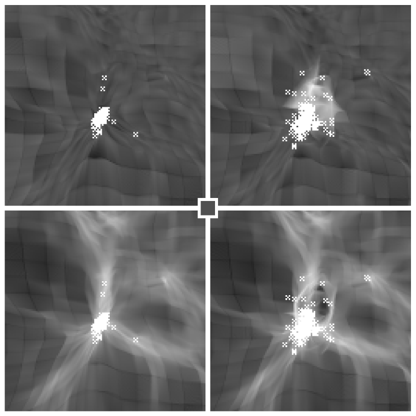
Figure 14: A slice of the gas density (lower row) and the gas temperature (upper row) of comoving dimensions $200h^{-1}\mbox{\,kpc}\times 200h^{-1}\mbox{\,kpc}\times 15h^{-1}\mbox{\,kpc}$ around the disrupted object at $z=11$ for runs A1 (left column) and C1 (right column). Stars (i.e. SLH stellar particles) are shown by white symbols. The small square at the center mark the mean cosmic density for the density panels and $T=10^{3}\mbox{\,K}$ for the temperature panels. The color version of this plot is available online as explained in the Appendix B.

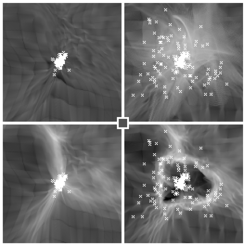
Figure 16: The same as Fig. 14 except at $z=9$.

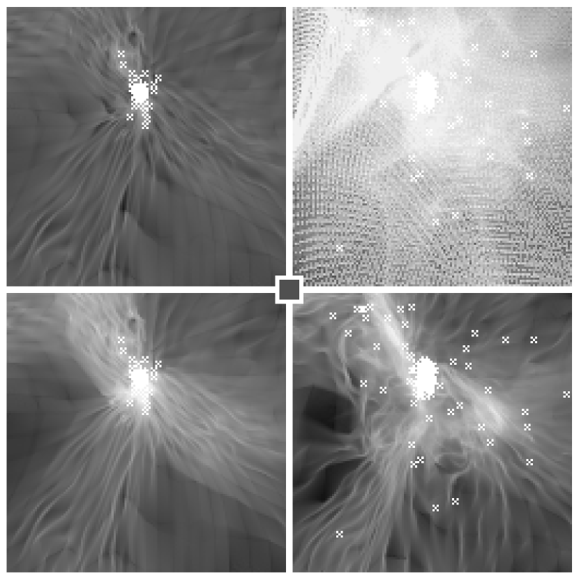
Figure 18: The same as Fig. 14 except at $z=7$. The upper right panel is of somewhat poorer quality than other panels because of incomplete rebinning.

Figures 14-18 serve to illustrate the process of gas disruption. These figures show a neighborhood of the object marked with a circle in Fig. 10. The scale of each panel is $200h^{-1}\mbox{\,kpc}\times 200h^{-1}\mbox{\,kpc}$ in comoving units. The upper panels show the gas temperature, and the lower panels show the gas density for the same object in runs A1 (the left panels) and C1 (the right panels). Fig. 14 shows the object at the moment of disruption, $z=11$, and Fig. 16 shows the same comoving volume at $z=9$. In order to illustrate the further evolution of this objects, runs A1 and C1 are continued until $z=7$, with Fig. 18 showing the same comoving volume at $z=7$. Stars are shown on the same plots with white stellar symbols.

The process of disruption started at $z=11$ with the ejection of the gas in the “north-east” direction (assuming that north is on the top of the figure), because the high-density filaments prevented the shock wave to expand into the north and east directions. The low density - high temperature region formed inside the shock wave. At a later time, $z=9$ (Fig. 16), the shock wave overcame the confining pressure of filaments and expanded in all directions; a very low gas density region formed around the proto-galaxy, which now contains almost entirely stars and the dark matter (not shown). The expanding shock wave snowplowed a large amount of external material, and secondary shock waves were propagating in all directions inside the expanding bubble. As it expanded and snowplowed the surrounding gas, the shock wave also managed to disrupt a small fraction of stars from the object; stars interact with the other matter only gravitationally, but since the gas constitutes some 15% of the total mass of the object (for a considered cosmological model), the mass of the expanding shell is not negligible, and some stars were disrupted from the proto-galaxy by the gravitational pull of the expanding shell. By $z=7$ (Fig. 18), the expanding shell dissolved and mixed with the surrounding IGM, heating the gas to much higher temperature than it would otherwise had.

For comparison, the left columns (run A1 without supernovae) show nothing even close to this spectacular activity.

An MPEG video of this process as well as color versions of Fig. 14-18 are available online as explained in Appendix B.

3.3 Metal Abundances in the Lyman-alpha Forest

Figure 20: The fraction of all peaks in the gas density which have the metallicity above the limiting value $Z_{\rm lim}=10^{-2}Z_{\odot}$ as a function of the cosmic gas density for runs A1 (solid lines), B1 (dotted lines), and C1 (dashed lines) as extrapolated to $z=3$. The upper scale shows the average column density of a Lyman-alpha forest line arising from a respective density peak (Hui et al. 1996). Points with errorbars are observational data from Womble et al. (1995) and Songaila & Cowie (1996) (the data point from Womble et al. (1995) is corrected by 17% for $Z_{\rm lim}=10^{-2}Z_{\odot}$ from their value of $Z_{\rm lim}=10^{-2.3}Z_{\odot}$ using the dependence of the fraction of all peaks above $Z_{\rm lim}$ from run A1).

While both the theoretical modelling and the observations of the metallicity of the Lyman-alpha Forest are still in the developing stages, it is still instructive to make a rough comparison of the results of simulations with the observational data from Womble et al. (1995) and Songaila & Cowie (1996). As was demonstrated by Hui et al. (1996), most of the Lyman-alpha lines with column densities below about $10^{16}\mbox{\,cm}^{-2}$ are arising from the peaks in the line-of-sight distribution of the cosmic gas density. Figure 20 shows by the bold lines the fraction of all one-dimensional density peaks (i.e. peaks along any one of three directions) with the metallicities in excess of 1% solar as a function of the peak density at $z=3$. Three almost coinciding lines correspond to three runs: A3 (the solid line), B3 (the dotted line), and C3 (the dashed line). Since all three runs were stopped at $z=4$, I have extrapolated the metallicity distributions from those three runs to $z=3$.

Since the density of a peak strongly correlates with the column density of a Lyman-alpha line, it is possible to establish a one-to-one correspondence between the peak density and the column density of the absorption line. Respective column densities are presented on the upper scale in Fig. 20 for a considered cosmological model (the correspondence between the peak density and the column density of a Lyman-alpha line depends on cosmological parameters). Solid dots with errorbars are data from Womble et al. (1995) (the leftmost point) and from Songaila & Cowie (1996). Since Womble et al. (1995) quote results for the limiting metallicity of $10^{-2.3}Z_{\odot}$, I have corrected their value for the limiting metallicity of 1% solar using the dependence of $f(Z>Z_{\rm lim})$ on $Z_{\rm lim}$ as derived from run A3 (by 17% percent). A somewhat arbitrary 25% errorbar was added to each data point.

One can note that the agreement between the observations and the simulations is pretty good, taking into account that no fitting has been performed to achieve this agreement. However, this agreement should only be considered as encouraging, but by no means definite agreement between the theoretical predictions and the observations. Since several theoretical uncertainties such as limited resolution of my simulations, scatter in the column density – peak density relation etc, are not included in the analysis, it remains to be seen if more accurate simulations (including generating synthetic Lyman-alpha spectra and analyzing them by fitting Voigt profiles) will confirm this agreement.

It also remains to be seen how sensitive this test is. Since the merging mechanism is the dominant metal transport mechanism in the IGM, and the amount of merging strongly depends on the amplitude of density fluctuations, one may expect that cosmological models with different amplitudes of density fluctuations on small scales (several hundred kpc) will have substantially different predictions for the fraction of Lyman-alpha lines above a certain metallicity as a function of a column density.

4 Conclusions

I have demonstrated by means of high resolution cosmological simulations that the dominant mechanism for transporting heavy elements from the high density cosmic gas (ISM) into the low density cosmic gas (IGM) is the merger mechanism as discovered by Gnedin & Ostriker (1996). Direct ejection of the interstellar gas by supernovae plays only a minor role in transporting metals into the IGM: for a realistic cosmological scenario (i.e. the one that has a reasonable amount of power on all relevant scales from the COBE scale all the way to the scale of about $100\mbox{\,kpc}$ probed by the low column density Lyman-alpha forest), and at the most favorable conditions, only a small fraction of all metals is directly expelled from proto-galaxies by supernovae, while most of all metals in the IGM are delivered by the merger mechanism. It does not mean that supernovae do not expel gas from proto-galaxies, and examples in Section 3.2 show that they indeed do. However, the main conclusion of this paper is that the other, merger mechanism is more important in transporting metals into the IGM (in particularly, because it is not a subject to the negative feedback process), and ignoring it in computing the metal transport rate in the IGM is inadequate.

As the result, the metallicity distribution in the IGM is highly inhomogeneous, in agreement with conclusions by Rauch et al. (1996) and Hellsten et al. (1996).

The metallicity distribution of Lyman-alpha absorbers as a function of their column density is in excellent agreement (subject to the unknown uncertainty due to the limitations of theoretical modelling) with the observational data from Womble et al. (1995) and Songaila & Cowie (1996).

Apparently, the effect of the supernovae depends on the star formation rate. One may therefore that the star formation rate can be underestimated in the simulations, thus leading to a erroneous conclusion that supernovae are not efficient in expelling metals from the ISM. While details of the specific implementation of star formation in the simulations reported on here can be found in Gnedin (1996), I note here that the algorithm adopted in the simulation assumes that the star formation occurs on the dynamical time in the rapidly cooling gas at a rate, which, if being continued until $z=0$, would substantially overpredict the stellar mass density in the universe at the current epoch. Thus, the star formation rate in the simulations, as all other relevant parameters, is pushed to the reasonable extreme in order to maximize the effect of supernovae. And still, even in the most favorable conditions, supernovae do not contribute significantly to the metal transport rate into the IGM at high redshift ($z\mathrel{\mathchoice{\vbox{\offinterlineskip\halign{\hfil$\reset@font\displaystyle#$\hfil\cr<\cr\sim\cr}}}{\vbox{\offinterlineskip\halign{\hfil$\reset@font\textstyle#$\hfil\cr<\cr\sim\cr}}}{\vbox{\offinterlineskip\halign{\hfil$\reset@font\scriptstyle#$\hfil\cr<\cr\sim\cr}}}{\vbox{\offinterlineskip\halign{\hfil$\reset@font\scriptscriptstyle#$\hfil\cr<\cr\sim\cr}}}}4$).

This conclusion is only relevant in the range of redshifts simulated in this paper, and for the class of cosmological models whose properties are similar to the LCDM model considered here. The current work makes no predictions about the relative importance of supernova driven winds at lower redshifts, where higher star formation rate and lower density of the cosmic gas in the virialised objects may lead to enhanced role of supernova driven outflows.

As a side note, I mention here that since the merging mechanism works irrespectively of the binding energy of a collapsed object, merging in clusters of galaxies at the current epoch also ejects metals in the IGM. Thus, I can make a prediction that, if the conclusions of this paper are indeed correct, the mean metallicity of the IGM at the current epoch can easily be as high as several percent, or even 10% of solar.

I am very grateful to Chris McKee for his numerous discussions with me and explanations of the physics of the multi-phase interstellar medium. I thank M. Rees, J. Silk, J. Ostriker, A. Dekel, S. Zepf, M. Steinmetz, and J. Miralda-Escudé for valuable comments. The manuscript has been substantially improved by comments and suggestion by the anonymous referee. This work was supported by the UC Berkeley grant 1-443839-07427. Simulations were performed on the NCSA Power Challenge Array under the grant AST-960015N and on the NCSA Origin2000 mini-supercomputer under the grant AST-970006N.

A Incorporating the Multi-Phase Interstellar Medium into a Cosmological Simulation

As has been shown by Cioffi et al. (1988), a supernova remnant radius $R_{S}$ in the pressure driven snowplow stage (when radiative losses set in) is given by the following expression:

$$R_{S}=25.7\mbox{\,pc}{E_{51}^{31/98}\over\xi^{5/98}n_{0}^{18/49}v_{100}^{3/7}},$$ (A1)

where $E_{51}$ is the energy of the supernova remnant in units of $10^{51}\mbox{\,erg}$, $n_{0}$ is the ambient hydrogen density in units of $1\mbox{\,cm}^{-3}$, $v_{100}$ is the shock velocity $v_{S}$ in units of $100\mbox{\,km}/\mbox{\,s}$, and

• $\displaystyle\hskip 0.0pt{\xi=\min\left(Z/Z_{\odot},3\times 10^{-3}n_{0}^{1/2}E_{51}^{1/4}\right),}$

as shown by Cioffi & Shull (1991). This radius is reached at the time $t_{S}$ after the explosion,

$$t_{S}=7.57\times 10^{4}\mbox{\,ys}{E_{51}^{31/98}\over\xi^{5/98}n_{0}^{18/49}v_{100}^{10/7}}.$$ (A2)

For the very low density ambient medium $n_{0}<n_{\rm crit}$, when radiative there are no losses, where

• $\displaystyle\hskip 0.0pt{n_{\rm crit}=2.8\times 10^{-3}\mbox{\,cm}^{-3}{v_{100}^{7}\over\xi^{3/2}E_{51}^{1/2}},}$

the supernova remnant radius is given by the following expression:

$$R_{S}=27.8\mbox{\,pc}{E_{51}^{1/3}\over n_{0}^{1/3}v_{100}^{2/3}}.$$ (A3)

The volume fraction $f_{\rm hot}$ of the ISM occupied by the supernova remnants is determined by the porosity $Q$,

• $\displaystyle\hskip 0.0pt{f_{\rm hot}=1-\exp(-Q),}$

where (McKee 1990; Silk 1996)

$$Q=\mbox{$\nu$}{1\over m_{\rm SN}}{d\rho_{*}\over dt}.$$ (A4)

Here $\nu$ is the 4-volume of the supernova remnant in the space-time, $d\rho_{*}/dt$ is the rate of star formation, and $m_{\rm SN}$ is the mass in stars formed per supernova. The 4-volume of the supernova remnant is given by the following expression:

$$\mbox{$\nu$}=q{4\pi\over 3}R_{S}^{3}t_{S},$$ (A5)

where a dimensionless parameter $q$ depends on the time-evolution of the supernova remnant.

I now assume that the remnant evolution terminates at the shock velocity $v_{\rm term}$. If $v_{term}=\beta c_{S}$, where $c_{S}$ is the sound speed of the ambient ISM, and $\beta$ is a parameter of order unity (Cioffi et al. 1988), then the 4-volume of the supernova remnant until the moment of maximum expansion is (McKee 1990)

• $\displaystyle\hskip 0.0pt{\mbox{$\nu$}_{1}={1\over 3\eta+1}{4\pi\over 3}R_{S}^{3}t_{S},}$

where $\eta=0.3$ is the power-law index of the expansion law, $R_{S}\sim t_{S}^{\eta}$. Comparing to equation (A5), I get $q_{1}=1/(3\eta+1)$. However, in this case one must also account for the contraction phase, which gives $q_{2}=1/(4\eta)$ (McKee 1990). The total $q$ in this case (which I will call Case A hereafter) is

• $\displaystyle\hskip 0.0pt{q_{A}={1\over 3\eta+1}+{1\over 4\eta}.}$

The volume of the ISM occupied by the supernova remnants contains hot ionized gas, and, therefore, no stars can form inside the supernova bubbles. However, as was shown by Shull & McKee (1979), a supernova remnant shock fails to ionize the ambient medium with the solar metallicity at the shock velocities below about $90\mbox{\,km}/\mbox{\,s}$. In this case the interstellar gas snowplowed by the supernova shock with a lower velocity will not be ionized and may form stars even if it located inside the supernova remnant. In order to account for this possibility, I consider $v_{term}$ as a free parameter, not necessarily close to the sound speed of the ambient ISM. Obviously, in no case can $v_{\rm term}$ be smaller than $\beta c_{S}$, but it can be larger. In the latter case (Case B) the contraction phase is not counted as being a part of hot ISM, and

• $\displaystyle\hskip 0.0pt{q_{B}={1\over 3\eta+1}.}$

Supernova remnants affect the ambient medium in two ways: they exert an addition pressure on the ambient gas, and, when they terminate, they deposit the rest of their mechanical energy that was not cooled off, into the ambient ISM. The pressure jump at the shock wave is

• $\displaystyle\hskip 0.0pt{{\Delta P\over P_{0}}={2\gamma\over\gamma+1}\left({\cal M}^{2}-1\right),}$

where $\gamma$ is the polytropic index for the gas, and ${\cal M}$ is the Mach number of the shock,

• $\displaystyle\hskip 0.0pt{{\cal M}={v_{\rm term}\over c_{S}}.}$

For the power-law expansion law the shock velocity changes as $t^{\eta-1}$, and the average relative excess pressure a supernova remnant exerts on the ambient ISM over its lifetime is

$${\Delta P\over P_{0}}={4\pi\over 3\mbox{$\nu$}}\int R_{S}(t)^{3}{2\gamma\over\gamma+1}\left({\cal M}(t)^{2}-1\right)dt={2\gamma\over\gamma+1}{p\over q},$$ (A6)

where dimensionless parameter $p$ is different for cases A and B:

Case A:

$\displaystyle p_{A}={1\over 5\eta-1}-{1\over 3\eta+1}$,

Case B:

$\displaystyle p_{B}={1\over 5\eta-1}\left(v_{\rm term}\over\beta c_{S}\right)^{2}-{1\over 3\eta+1}$.

Note, that in the latter case $p_{B}$ (and, therefore, the excess pressure) can be very large if $v_{\rm term}\gg\beta c_{S}$.

After the supernova remnant dies, the rest of its energy is deposited in the ISM as thermal heating. The total thermal energy density deposited in the ISM by a supernova remnant is then

$${\Delta U\over U_{0}}={2\gamma\over\gamma+1}\left({\cal M}^{2}-1\right)\left(1+{(\gamma-1)({\cal M}^{2}-1)\over 2+(\gamma-1){\cal M}^{2}}\right),$$ (A7)

where $U_{0}$ is the energy density in the ambient medium.

Equations (A4), (A6), and (A7) can now be incorporated in the SLH-P³M code. Let the subscript 0 denotes quantities that would be computed by the code in the absence of supernova, i.e. when $f_{\rm hot}=0$. The hydrodynamic gas pressure is corrected as $P=P_{0}+\Delta Pf_{\rm hot}$, the star formation rate is reduced by a factor of $f_{\rm hot}$,

$${d\rho_{*}\over dt}=\left(d\rho_{*}\over dt\right)_{0}(1-f_{\rm hot}),$$ (A8)

and the thermal energy is ejected in the gas at the rate

• $\displaystyle\hskip 0.0pt{\left(dU\over dt\right)_{SN}=\Delta Uf_{\rm hot}{1\over m_{SN}}{dm_{*}\over dt}.}$

I would like to point out here that the reduction in the star formation rate itself depends on the porosity of the IGM, which itself depends on the star formation rate. This mutual dependence works as a powerful feedback mechanism.

The last undefined parameter in this treatment is $m_{SN}$, the total mass in stars formed per supernova. For a solar neighborhood (or Miller-Scalo) IMF this value is $m_{SN}=250{\rm M}_{\odot}$. I introduce a new parameter, $f_{\rm IMF}$, defined as

• $\displaystyle\hskip 0.0pt{f_{\rm IMF}={250{\rm M}_{\odot}\over m_{SN}},}$

to account for possible deviations from the Miller-Scalo IMF. As argued by Silk (1996), a value of $f_{\rm IMF}\sim 4$ is required in order to account for all metals in the clusters of galaxies.

Finally, since $p_{B}$ (and, therefore, $\Delta P$) increases with increasing the termination velocity $v_{\rm term}$, one may imagine that the effect of supernovae may be increased indefinitely by increasing $v_{\rm term}$. However, since both $R_{S}$ and $t_{S}$ decrease with increasing $v_{\rm term}$, the porosity of the ISM decreases with increasing $v_{\rm term}$ as $Q\sim v_{\rm term}^{-19/7}$ (or $Q\sim v_{\rm term}^{-24/7}$ for $n_{0}<n_{\rm crit}$). Therefore, for a sufficiently large $v_{\rm term}$, when the porosity is small, $f_{\rm hot}=Q\sim v_{\rm term}^{-19/7}$ and the total correction to the gas pressure (and to the thermal energy) decreases with increasing $v_{\rm term}$ as $\Delta P\sim v_{\rm term}^{-5/7}$. There is therefore a value for $v_{\rm term}$ when the effects of supernova on the ambient ISM is maximal.

B Attachments

Additional illustrations to this paper are available online at the URL: http://astron.berkeley.edu/~gnedin/metigm.html. They include:

• color versions of Fig. 14-18;

• color versions of Fig. 14-18 but with the slice width of $1h^{-1}\mbox{\,kpc}$ instead of $15h^{-1}\mbox{\,kpc}$;

• an MPEG video of the evolution of the object discussed in §3.2;

• a color image showing the merging mechanism at work.

References

- \citename Bi, H. G., Davidsen, A. F. 1996, ApJ, in press (astro-ph 9611062)
- \citename Cen, R. Y., Miralda-Escudé, J., Ostriker, J. P., Rauch, M. R. 1994, ApJ, 437, L9
- \citename Cen, R. Y., Ostriker, J. P. 1992, ApJ, 399, L113
- \citename Cioffi, D. F., McKee, C. F., Bertschinger, E. 1988, ApJ, 334, 252
- \citename Cioffi, D. F., Shull, J. M. 1991, ApJ, 367, 96
- \citename Couchman, H. M. P., Rees, M. J. 1986, MNRAS, 221, 53
- \citename Dekel, A., Silk, J. 1986, ApJ, 303, 39
- \citename Gnedin, N. Y. 1995, ApJS, 97, 231
- \citename Gnedin, N. Y. 1996, ApJ, 456, 1
- \citename Gnedin, N. Y., Bertschinger, E. 1996, ApJ, 470, 115
- \citename Gnedin, N. Y., Ostriker, J. P. 1996, ApJ, in press (astro-ph 9612127)
- \citename Haiman, Z., Rees, M. J., & Loeb, A. 1996, ApJ, submitted (astro-ph 9608130)
- \citename Hellsten, U., Dave, R., Hernquist, L., Weinberg, D., Katz, N. 1997, ApJ, submitted (astro-ph 9701043)
- \citename Hernquist, L., Katz, N., Weinberg, D. H., Miralda-Escudé, J. 1996, ApJ, 457, L51
- \citename Hui, L., Gnedin, N. Y., Zhang, Y. 1996, ApJ, in press (astro-ph 9608157)
- \citenameKatz, Weinberg, & Hernquist1996 Katz, N., Weinberg, D. H., Hernquist, L. 1996, ApJS, 105, 19
- \citename McKee, C. F. 1990, in The Evolution of the Interstellar Medium, ASP Conference Series, 12, 3
- \citename Miralda-Escudé, J., Cen, R., Ostriker, J. P., Rauch, M. 1996, ApJ, 471, 582
- \citename Miralda-Escudé, J., Rees, M. J. 1997, ApJ, submitted (astro-ph 9701093)
- \citename Navarro, J. F., White, S. D. M. 1993, MNRAS, 265, 271
- \citename Ostriker, J. P., Gnedin, N. Y. 1996, ApJ, 472, L63
- \citename Petitjean, P., Mucket, J. P., & Kates, R. E. 1995, A&A, 295, L9
- \citename Rauch, M., Haehnelt, M. G., Steinmetz, M. 1996, ApJ, submitted (astro-ph 9609083)
- \citename Silk, J. 1996, ApJ, in press (astro-ph 9612177)
- \citename Shull, J. M., McKee, C. F. 1979, ApJ, 227, 131
- \citename Shull, J. M., Silk, J. 1981, ApJ, 249, 26
- \citename Songaila, A., Cowie, L. L. 1996, AJ, 112, 335
- \citename Tytler, D., Burles, S. 1996, to appear in Proc. International Symposium on ”Origin of Matter and Evolution of Galaxies in the Universe”, Atami, Japan (astro-ph 9606110)
- \citename Wadsley, J. W., Bond, J. R. 1996, to appear in Proc. 12th Kingston Meeting, Halifax, Canada (astro-ph 9612148)
- \citename Womble, D. S., Sargent, W. L. W., Lyons, R. S. 1995, astro-ph 9511035
- \citename Zhang, Y., Anninos, P., Norman, M. L. 1995, ApJ, 453, L57