Searching for Machos (and other Dark Matter Candidates)

 in a Simulated Galaxy

Lawrence M. Widrow

Department of Physics

Queen’s University, Kingston, K7L 3N6, CANADA

and

 John Dubinski

Canadian Institute for Theoretical Astrophysics

University of Toronto, Toronto, M5S 1A1, CANADA

We conduct gravitational microlensing experiments in a galaxy taken from a cosmological N-body simulation. Hypothetical observers measure the optical depth and event rate toward hypothetical LMCs and compare their results with model predictions. Since we control the accuracy and sophistication of the model, we can determine how good it has to be for statistical errors to dominate over systematic ones. Several thousand independent microlensing experiments are performed. When the “best-fit” triaxial model for the mass distribution of the halo is used, the agreement between the measured and predicted optical depths is quite good: by and large the discrepancies are consistent with statistical fluctuations. If, on the other hand, a spherical model is used, systematic errors dominate.

Even with our “best-fit” model, there are a few rare experiments where the deviation between the measured and predicted optical depths cannot be understood in terms of statistical fluctuations. In these experiments there is typically a clump of particles crossing the line of sight to the hypothetical LMC. These clumps can be either gravitationally bound systems or transient phenomena in a galaxy that is still undergoing phase mixing. Substructure of this type, if present in the Galactic distribution of Machos, can lead to large systematic errors in the analysis of microlensing experiments.

We also describe how hypothetical WIMP and axion detection experiments might be conducted in a simulated N-body galaxy.

1 Introduction

Four years ago the MACHO (Alcock et al. 1993) and EROS (Aubourg et al. 1993) collaborations announced candidate gravitational microlensing events toward the Large Magellanic Cloud (LMC) demonstrating the viability of a new and potentially powerful probe of dark matter in the Galactic halo. Microlensing experiments (Paczyński 1986; Griest 1991) are sensitive to any object that is smaller than its Einstein radius (in the halo, these objects are known as Machos for massive compact halo objects) and therefore complement direct observations, which survey the visible content of the Galaxy, and dynamical studies, which measure the total mass density. Unfortunately, microlensing experiments are subject to a number of limitations which make interpretation of their results rather difficult. First, microlensing events are extremely rare and it is necessary to monitor $O(10^{6})$ stars in order to get just a few events per year. This has restricted present day searches to regions of the sky where there are dense concentrations of stars. Indeed the only published microlensing events that can be associated with halo objects have been toward the Large and Small Magellanic Clouds (Alcock et al. 1993, 1995, 1996, 1997b; Aubourg et al. 1993). Microlensing experiments, with only one or two lines of sight, tell us little about the structure of the halo and, more to the point, are sensitive to potentially large systematic errors due to our incomplete knowledge of the halo’s structure. Moreover, because of the small number of events, there are large statistical uncertainties. Finally, present day experiments are unable to determine unambiguously the mass and velocity of a given lens. Despite these limitations the MACHO collaboration estimates, from the two-year data set, that $\sim 50\%$ or more of the mass in the halo within $50{\rm\,kpc}$ is composed of $\sim 0.5\,M_{\odot}$ objects (Alcock et al. 1996). If true, these results would have important implications for cosmology, galaxy formation, and star formation.

The mass density in Machos is determined by comparing the observed number of events with the number predicted for a particular model of the Galaxy. Potential systematic errors are estimated by seeing how the predicted number of events varies for different “reasonable” Galactic models. This strategy, however, is hindered by our limited ability to construct and analyze the full complement of acceptable models. In particular, the models used to analyze MACHO’s results do not generally include triaxiality, velocity space anisotropy, and substructure, all of which are expected in the real distribution of Machos.

In this paper we propose an alternative approach to understanding gravitational microlensing experiments. Microlensing experiments are conducted in a halo taken from a cosmological N-body simulation. Hypothetical observers make measurements of the optical depth and event rate and compare their results with model predictions much as real observers would. We can perform a large number of microlensing experiments on a single N-body halo by simply changing the positions of the observer and LMC. Since we control the accuracy and sophistication of the model, we can determine how good it has to be for statistical errors to dominate over systematic ones.

Our intention is not to create an N-body realization of the Milky Way Galaxy. Indeed our galaxy bears little resemblance to the Milky Way. Moreover, the simulation assumes a cold dark matter universe which may not be appropriate if a significant fraction of the dark matter is composed of Machos. However the distribution of particles in the simulated galaxy does exhibit the general characteristics (e.g., triaxiality, substructure) that one expects in a realistic distribution of Machos. We can therefore test how well theory agrees with observation when these features are not fully taken into account.

We find that a simple triaxial model, with the axial ratios and density profile determined from the simulation, provides excellent agreement between measured and predicted optical depths. In all but a few rare experiments the discrepancies are consistent with the statistical fluctuations that one would expect had the particles been chosen at random from the model distribution function. If instead an axisymmetric spheroidal model is used, systematic errors become important. And if a spherical model is used, systematic errors dominate.

Microlensing experiments are also sensitive to the velocity space distribution of the Machos. If the velocities assumed in the model are too high, for example, one will tend to overestimate the mass of individual Machos and their density. To study this, we measure the event rate in the simulated galaxy and compare with the expected rate assuming different models for the velocity distribution.

The visible parts of galaxies display substructure such as globular clusters and dwarf galaxies. Substructure is also likely to exist in the distribution of dark matter especially in hierarchical clustering models of galaxy formation. Microlensing experiments are especially sensitive to substructure in the Galaxy: If we are unlucky, a clump of Machos will be passing between us and the LMC, biasing our estimates for the density of Machos in the halo (Maoz 1994; Wasserman & Salpeter 1994; Metcalf & Silk 1996, Zhao 1996). Our simulated microlensing experiment shows just such an effect. Even with our best-fit triaxial model, there are a few lines of sight in which the measured optical depth is significantly higher than what is predicted. A close inspection of these lines of sight reveal that substructure in the halo is often the cause of the discrepancy.

In Section II we survey the types of models previously considered for the distribution of Machos. The methods used to conduct microlensing experiments in an N-body galaxy are developed in Section III. Our the results are presented in Section IV. In Section V we describe how hypothetical terrestrial dark matter detection experiments can be performed in an N-body galaxy. Section VI presents a summary of our results and some concluding thoughts.

2 Previous Analyses of the MACHO Experiment

A model for Machos must specify their distribution in mass, configuration space, and velocity space. The “standard” halo model, used as a benchmark by the MACHO collaboration, assumes that all of the Machos have the same mass, that their velocities are isotropic and Maxwellian, and that their density corresponds to that of a cored isothermal sphere (Griest 1991; Alcock et al. 1995, 1996). This implies a distribution function (DF) of the form:

$$f({\bf x},{\bf v})=\rho({\bf x})F({\bf v})$$ (1)

where

$$\rho({\bf x})=\frac{{\cal F}v_{\infty}^{2}}{4\pi G}\frac{1}{r^{2}+r_{c}^{2}}$$ (2)

and

$$F({\bf v})=\frac{1}{\left(\pi v_{\infty}^{2}\right)^{3/2}}\exp{\left(-\frac{v^{2}}{v_{\infty}^{2}}\right)}~{}.$$ (3)

$r_{c}$ is the core radius, $\cal F$ is the fraction of the halo in Machos, and $v_{\infty}$ is the asymptotic circular speed of the total halo. In the standard model, $r_{c}=5{\rm\,kpc}$ and $v_{\infty}=220{\rm\,km/sec}$ while $\cal F$ and $M_{0}$ are left as free parameters. It is a likelihood analysis of this 2-parameter model that leads to the MACHO collaboration’s estimates for the mass and density of Machos in the Galaxy.

The DF described above represents a highly idealized Macho halo. Deviations between the model and the actual distribution of Machos may introduce significant systematic errors in the analysis of a microlensing experiment. One can estimate these errors by considering alternative models. Several groups, for example, have considered models in which the assumption of spherical symmetry is relaxed. For the most part these groups have focused on the seemingly reasonable possibility that the halo is an axisymmetric oblate spheroid (Sackett & Gould 1993; Friemann & Scoccimarro 1994; Gates, Gyuk, & Turner 1995; Alcock et al. 1995, 1996). Models of this type can be constructed by replacing $r^{2}$ in Eq.(2) by $m^{2}\equiv x^{2}+y^{2}+z^{2}/q^{2}$ where $q$ is the axial ratio ($<1$ for oblate spheroids) and by multiplying $\rho$ by $\lambda(q)\equiv\sqrt{1-q^{2}}/\left(q{\rm\,arccos{q}}\right)$. Interestingly enough, the optical depth and event rate do not change much as $q$ varies from $0.4$ (E6 oblate) to $1.0$ (spherical). This is because two competing effects cancel approximately. As the model halo is made more oblate, the central density must be increased if $v_{\infty}$ is to be kept fixed. This tends to increase the optical depth. At the same time our line of sight to the LMC passes through less halo material which tends to reduce the optical depth.

The results for flattened halos have lead to the conjecture that the total inferred mass of Machos within $50{\rm\,kpc}$ is relatively independent of the assumed model ( Gates, Gyuk, & Turner 1995; Alcock et al. 1996). However there is little direct evidence to suggest that the dark Galactic halo is axisymmetric and oblate. Observational clues about the shape of the dark Galactic halo come from models of the metal-poor stellar halo (Gilmore, Wyse, & Kuijken 1989; van der Marel 1991), the outer satellites and globular clusters (Hartwick 1996), and HI gas near the Galactic plane (Merrifield & Olling 1997). The results are highly model dependent and somewhat ambiguous leaving open the possibility that the Galactic halo is prolate or triaxial.

Numerical experiments may provide the best hope for understanding the structure of dark halos. The halos found in N-body simulations of dissipationless gravitational collapse are generally triaxial with a slight preference to be prolate rather than oblate (Dubinski & Carlberg 1991; Warren et al. 1992; see also the simulation discussed below). The inclusion of dissipational matter, which tends to settle into a thin disk, will change these results somewhat typically driving systems to become more oblate (Katz and Gunn 1991; Dubinski 1994) though still generally triaxial. And there are exceptions (Evrard, Summers, and Davis 1994) suggesting that some halos may be prolate-triaxial even when dissipational matter is included. With this in mind Holder & Widrow (1996) have calculated the optical depth and event rate for prolate halos. For these models the central density is lowered relative to what it would be in a spherical model. This effect dominates so that predicted optical depth is reduced by a significant amount.

Galactic microlensing experiments are also sensitive to the velocity space distribution of the Machos. If, for example, Machos are preferentially on radial orbits, than the timescale for events would be systematically longer than what would be expected assuming an isotropic velocity distribution (Evans 1996). The triaxial N-body halos discussed above are supported by anisotropic velocity dispersion which can affect the event rate and event duration (Holder & Widrow 1996; Evans 1996).

One criticism of the models discussed above is that they do not represent true equilibrium systems: with the exception of the special case $r_{c}=0,~{}q=1$ (the singular isothermal sphere) a distribution function given by Eqs. (1-3) does not satisfy the time-independent collisionless Boltzmann equation. Evans and Jijina (1994) have attempted to address this concern by using the so-called power-law models for the Macho DF. These models are constructed from simple power-law functions of the energy and angular momentum and therefore automatically describe equilibrium systems. Their main advantage is that they are simple and analytic making lensing calculations relatively easy. They do have certain drawbacks. First, while the equipotential surfaces are spheroidal, the isodensity surfaces are dimpled at the poles. Second, once the disk is included, the models no longer describe self-consistent equilibrium systems.

Finally, several groups have considered the implications of subgalactic clustering in the distribution of Machos (Maoz 1994; Wasserman & Salpeter 1994; Metcalf & Silk 1996; Zhao 1996). In general these analyses make ad hoc assumptions about the distribution and structure of Macho clusters.

3 Preliminaries

3.1 The Simulated Halo

Our halo is taken from a collisionless N-body simulation of a cold dark matter (CDM) universe. Of course Machos are, in all likelihood, baryonic suggesting that a simulation of a baryon dominated universe might be more appropriate. However once Machos form they are essentially collisionless. We therefore expect that a Macho halo will exhibit triaxiality, velocity space anisotropy, and substructure, much like a CDM halo.

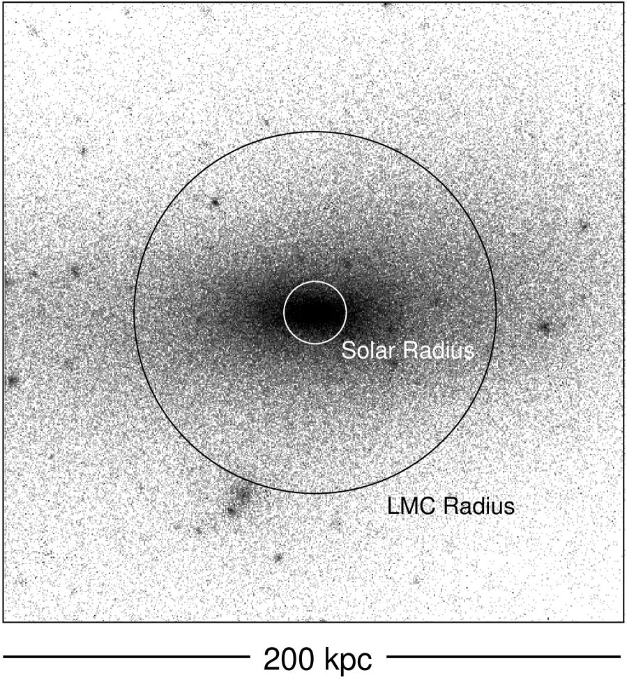
Figure 1: The N-body galaxy in projection. This projection is along the intermediate axis of the galaxy so that its prolate nature is readily apparent. The inner circle represents the positions of hypothetical observers; the outer circle represents the positions of hypothetical LMCs.

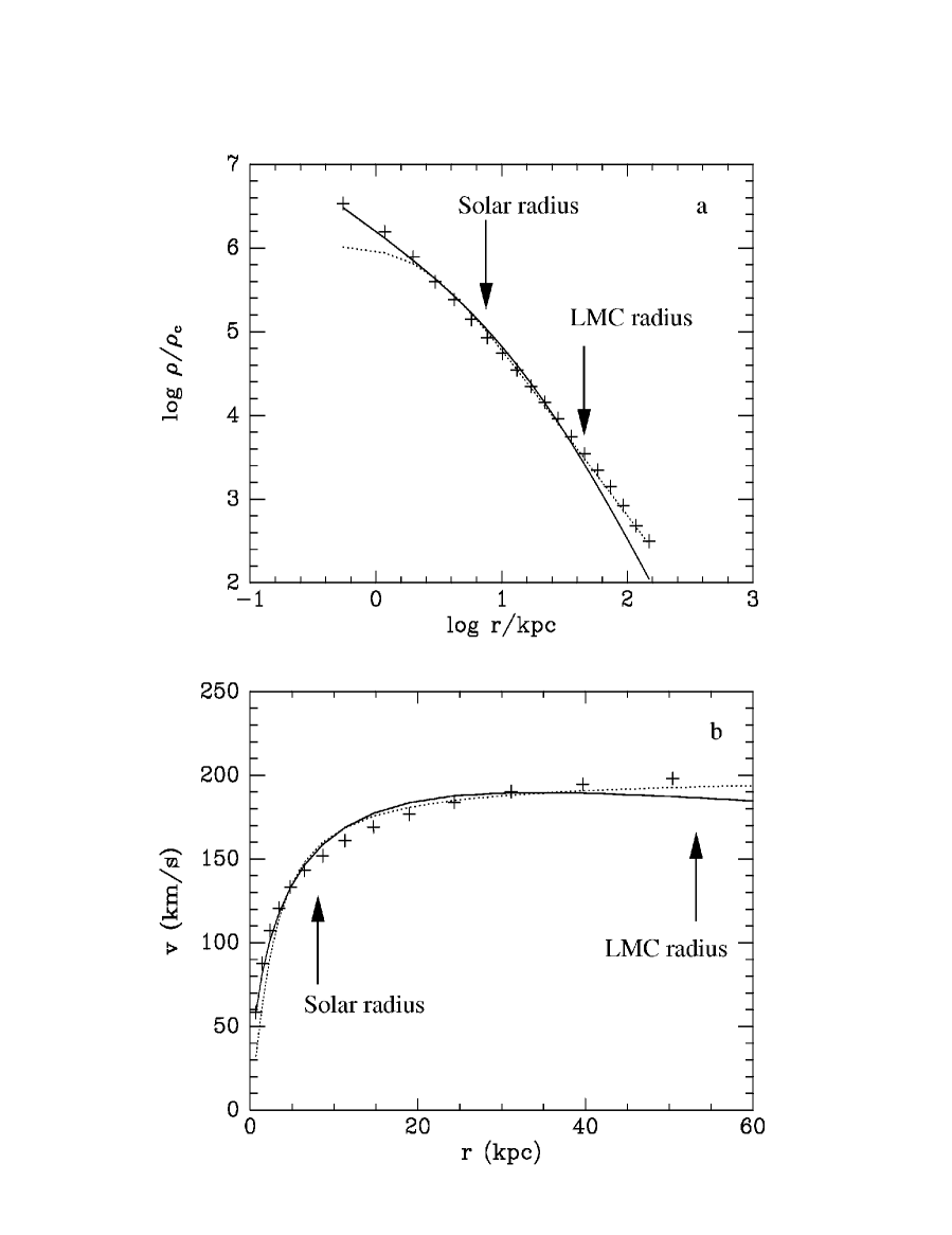
Figure 2: (a) Density profile and (b) rotation curve for the simulated halo. Crosses represent the spherically averaged density and circular rotation speed for the halo. The solid lines are for the NFW profile discussed in the text. The dotted lines are for the best-fit cored isothermal sphere ($r_{c}=2.4{\rm\,kpc}$, $v_{\infty}=200{\rm\,km/sec}$).

The halo is extracted from cosmological collapse simulation run with a parallel treecode on the Pittsburgh Cray T3E (Dubinski 1996). The halo is comprised of roughly 700,000 particles within the virial radius though there are only 260,000 particles within the radius of the LMC (Figure 1). Each particle has a mass $M_{\rm P}=2.7\times 10^{6}\,M_{\odot}$. The experiments are conducted at two different epochs corresponding to ages of $9.7\,{\rm Gyr}$ and $16.0\,{\rm Gyr}$. The results are essentially the same for the two time frames and we present only those from the latter. The galaxy is prolate-triaxial and has a relatively flat rotation curve out to large radii (Figure 2). We model the mass distribution of the galaxy by assuming that isodensity surfaces are ellipsoidal so that $\rho=\rho(m)$ where $m^{2}=x^{2}+y^{2}/q_{1}^{2}+z^{2}/q_{2}^{2}$ provided we have chosen the axes to coincide with the principle axes of the Galaxy. The density profile is fit to an NFW profile (Navarro, Frenk, & White 1996):

$$\rho(m)~{}=~{}\frac{M_{s}}{4\pi q_{1}q_{2}}\,\frac{1}{m\left(m+a_{s}\right)^{2}}$$ (4)

where $M_{s}$ is equal to the mass inside an ellipsoidal radius $m=3a_{s}$. $M_{s},\,a_{s},\,q_{1},$ and $q_{2}$ determined directly from the simulation. We also use less sophisticated models, specifically, a spheroidal model ($q_{1}=q_{2}=0.5$) and a spherical one. The model parameters are summarized in Table 1.

Model	$q_{1}$	$q_{2}$	$M_{s}(10^{11}M_{\odot})$	$a_{s}({\rm\,kpc})$
I (triaxial)	0.55	0.44	5.2	21.4
II (spheroidal)	0.5	0.5	5.2	21.2
III (spherical)	1.0	1.0	6.5	15.9

Table 1: Model parameters

$M_{s}$ and $a_{s}$ depend sensitively on the region of the halo used in the fit. In other words, Eq. (4) does not provide a very good global model for this particular galaxy. This is especially true for the $16\,{\rm Gyr}$ time frame where the halo is merging with a satellite. Of course, microlensing experiments only probe the region of the halo between the observer and the target stars (i.e., between $8.5{\rm\,kpc}$ and $50{\rm\,kpc}$) where the density profile is close to a power law. The parameters in Table 1 are chosen to fit the density profile in this region. In fact, any number of fitting formulae could be used. For example, a cored isothermal sphere (Eq. (2)) with $r_{c}=2.4{\rm\,kpc}$, ${\cal F}=1$, and $v_{\infty}=200{\rm\,km/sec}$ does just as well since the observer is outside the core radius and the LMC is inside the radius where the density profile becomes steeper than $r^{-2}$. In Figure 2 we show the circular rotation speed $v_{c}\,\left(\equiv(GM(r)/r)^{1/2}\right)$ for the halo, Model I, and the “best-fit” cored isothermal sphere.

A galactic coordinate system is set up in the usual way. Our hypothetical observer is at the origin, the center of the galaxy is on the $y$-axis a distance $r_{s}=8.5{\rm\,kpc}$ away, and the $z$-axis points “north”. The hypothetical LMC is at galactic coordinates $(l,\,b)=(-32.8^{\circ},\,281^{\circ})$ a distance $L$ from the origin. For simplicity we assume that the hypothetical LMC, in projection as seen from the observer, is a circle of radius $R_{\rm LMC}$. The foreground of the LMC is a conical volume $\Omega$ with base diameter $2R_{\rm LMC}$ and height $L$.

Different realizations of the experiment are performed by varying the orientation of the halo keeping the observer, LMC, and center of the halo fixed. Since our halo does not have a disk, the observer is not constrained to any particular plane. We therefore have three degrees of freedom (the Euler angles) in choosing the orientation of the halo. Equivalently, we can imagine keeping the halo fixed and considering a family of hypothetical observers positioned on the surface of a sphere a distance $r_{s}$ from the center of the halo. The hypothetical LMCs lie on a concentric sphere of radius $\left(L^{2}-2r_{s}L\cos{b}\cos{l}+r_{s}^{2}\right)^{1/2}$ (Figure 1). For each observer, there is a circle of LMCs a distance $L$ away that have the correct orientation.

3.2 Optical Depth

The optical depth $\tau$ is the probability that light from a star in the LMC will be amplified by a factor $A$. This requires that a Macho pass within a distance $R=uR_{\rm E}$ from the line of sight where $u=2^{1/2}\left[A\left(A^{2}-1\right)^{-1/2}-1\right]^{1/2}$, $R_{\rm E}$ is the Einstein radius:

$$R_{\rm E}(z^{\prime})=9.65\times 10^{-8}\left(\frac{M}{M_{\odot}}\frac{L}{50{\rm\,kpc}}\frac{z^{\prime}\left(L-z^{\prime}\right)}{L^{2}}\right)^{1/2}{\rm\,kpc}~{},$$ (5)

and $z^{\prime}$ is the distance to the Macho. For definiteness we set $A=1.34~{}(u=1)$ and $L=50{\rm\,kpc}$. If all of the Machos have the same mass then $\tau$ is equivalent to the number of Machos in a tube (the so-called lensing tube) whose axis is the line of sight and whose radius is $R_{\rm E}$. The expectation value of $\tau$, given an analytic model for $f$, is

$$\langle\tau\rangle = \frac{1}{M}\int d^{3}{\bf x}\rho({\bf x})$$ (6)

$$= \frac{1}{M}\int_{0}^{L}dz^{\prime}\rho(z^{\prime})\pi R_{\rm E}^{2}(z^{\prime})$$ (7)

where $\rho({\bf x})=\int d^{3}{\bf v}f({\bf x},{\bf v})$. We also calculate $\sigma_{\tau}$, the standard deviation one expects for $\tau$ assuming particles are chosen at random from the model DF. The relevant equations for this are derived in the Appendix.

We can measure $\tau$ in our N-body halo by counting the number of particles in a lensing tube whose radius is given by Eq. (5) with $M=M_{\rm P}$. (Recall that, for fixed mass density in Machos, $\tau$ is independent of $M$.) Of course only a very small fraction of the tubes will contain a particle. We can mimic what is done in the MACHO experiment by counting the number of particles in a large number $(\sim 10^{6})$ of tubes each of which lies, more or less, in the volume $\Omega$. However, it is more efficient to use all of the particles in $\Omega$, weighting them by an appropriate geometric factor. To be precise we write the DF for our N-body galaxy as the sum of $\delta$-functions:

$$f=M_{\rm P}\sum_{i}\delta\left({\bf x}-{\bf x}_{i}\right)\delta\left({\bf v}-{\bf v}_{i}\right)$$ (8)

where $i$ labels the particles in the simulation. Substituting into Eq. (6) we have

$$\tau=\sum_{i}\left(\frac{R_{\rm E}(z_{i})}{\theta_{\rm LMC}z^{\prime}_{i}}\right)^{2}$$ (9)

where the sum is over all particles in $\Omega$ and we use $M=M_{\rm P}$ in calculating $R_{\rm E}$.

An alternative strategy is to replace $\Omega$ with a volume $\tilde{\Omega}$ whose shape is the same as that of a lensing tube. For example, we can choose $\tilde{\Omega}$ to be a tube of radius $R_{\rm tube}(z^{\prime})=2R_{\rm LMC}\left(z^{\prime}(L-z^{\prime})/L^{2}\right)^{1/2}$ so that the maximum radius of the tube is equal to the radius of the LMC. In this case all particles contribute equally to $\tau$ making it easy to visualize the phase space distribution of objects in the tube. Furthermore, near the observer, where the density of halo objects is presumably highest, $\tilde{\Omega}$ is fatter than $\Omega$. We therefore expect more objects in the tube and hence better statistics. The main disadvantage of this strategy is that it distorts the geometry of a realistic microlensing experiment. The angular diameter of $\tilde{\Omega}$ is $\tilde{\theta}=2\tan^{-1}\left((L-z^{\prime})/z^{\prime}\right)$ which is far too big near the observer. We will therefore use $\Omega$ to calculate the optical depth. However we use $\tilde{\Omega}$ to calculate the event rate where it is difficult to estimate statistical uncertainties when $\Omega$ is used (see Appendix and the next section).

3.3 Event Rate

In practice the expected number of events, $N_{\rm exp}$, is more useful than the optical depth when comparing predictions with observations. $N_{\rm exp}$ is given by

$$N_{\rm exp}=E\int_{0}^{\infty}\frac{d\Gamma}{d\hat{t}}\epsilon(\hat{t})d\hat{t}$$ (10)

where $\hat{t}=2R_{\rm E}/v_{\varpi}$ is the event duration, $v_{\varpi}$ is the magnitude of the transverse Macho velocity in the lensing tube rest frame, $\epsilon(\hat{t})$ is the detection efficiency, and $E$ is the “exposure” for the experiment given in units of “star-yr”. The differential event rate is given by

$$d\Gamma=\frac{1}{M}d\sigma d{\bf v}f({\bf x},{\bf v})v_{\varpi}\cos{\theta}$$ (11)

where $d\sigma=R_{\rm E}d\phi dz^{\prime}$ is a surface element on the lensing tube and $d^{3}{\bf v}=dv_{z^{\prime}}v_{\varpi}dv_{\varpi}d\theta$. Given an analytic function for $f$, the total event rate $\Gamma$ is found by integrating over ${\bf v}$ and $\sigma$. To calculate $d\Gamma/d\hat{t}$, the event rate as a function of event duration, we change variables from $v_{\varpi}$ to $\hat{t}$, differentiate with respect to $\hat{t}$, and integrate over the remaining variables.

If the velocities of the Machos are isotropic and Maxwellian (Eq. (3)) than the expectation values for $\Gamma$ and $d\Gamma/d\hat{t}$ are

$$\langle\Gamma\rangle=\frac{\pi^{1/2}v_{\infty}}{M}\int_{0}^{L}dz^{\prime}\rho(z^{\prime})R_{\rm E}(z^{\prime})$$ (12)

and

$$\left\langle\frac{d\Gamma}{d\hat{t}}\right\rangle=\frac{32}{\hat{t}^{4}Mv_{\infty}^{2}}\int_{0}^{L}\rho(z^{\prime})R_{\rm E}(z^{\prime})\exp{\left[-\frac{rR_{\rm E}^{2}(z^{\prime})}{\hat{t}^{2}v_{\infty}^{2}}\right]}dz^{\prime}~{}.$$ (13)

An expression for $\sigma_{\Gamma}$, the standard deviation for $\Gamma$ assuming particles are chosen at random from an analytic DF, is derived in the appendix.

Eq. (11) represents a flux of particles through a surface, something that is difficult to measure in an N-body simulation. To circumvent this problem we multiply both sides of Eq. (11) by $\varpi d\varpi$ where $\varpi$ is the distance from the axis of the lensing tube:

$$\varpi d\varpi d\Gamma=\frac{1}{M_{\rm P}}d^{3}{\bf x}d^{3}{\bf v}f({\bf x},{\bf v})v_{\varpi}\cos{\theta}R_{\rm E}(z^{\prime})~{}.$$ (14)

Substituting Eq. (8) for $f$ and integrating over the volume $\tilde{\Omega}$ yields an expression for $\Gamma$ that is directly applicable to an N-body galaxy:

$$\Gamma=\frac{2}{\pi}\sum_{i}\frac{R_{\rm E}(z_{i})v_{\varpi,i}}{R_{\rm tube}^{2}(z_{i})}~{}.$$ (15)

$d\Gamma/d\hat{t}$ is estimated by binning the events according to event duration.

3.4 An Illustrative Example

We illustrate the techniques developed above in a toy galaxy where the positions and velocities of the particles are chosen at random from a known analytic DF. For definiteness we assume that this DF is given by Eqs.(1-3) with ${\cal F}=1$, $v_{\infty}=200\,{\rm\,km/sec}$, and $r_{c}=5{\rm\,kpc}$. The galaxy is represented by 200,000 $M_{\rm P}=2.2\times 10^{6}M_{\odot}$ mass particles. 1000 individual microlensing experiments are performed, each of which assumes a different orientation for the galaxy. To be precise, let $(\alpha,\,\beta,\,\gamma)$ be the three Euler angles which describe the galaxy’s orientation. We take $10$ even steps in $\alpha$ (from $0$ to $2\pi$), $\cos{\beta}$ (from $-1$ to $1$), and $\gamma$ (from $0$ to $2\pi$). We choose $R_{\rm LMC}=4{\rm\,kpc}$. This is roughly a factor of two larger than the real LMC, a choice made to increase the number of particles in the experimental volume $\Omega$.

From the analytic DF we calculate $\langle\tau\rangle$, $\langle\Gamma\rangle$, and $\langle d\Gamma/d\hat{t}\rangle$ as well as $\sigma_{\tau}$ and $\sigma_{\Gamma}$. We next compute, for each experiment, the normalized errors

$$\varepsilon_{\tau}~{}=~{}\frac{\tau-\langle\tau\rangle}{\sigma_{\tau}}$$ (16)

$$\varepsilon_{\Gamma}~{}=~{}\frac{\Gamma-\langle\Gamma\rangle}{\sigma_{\Gamma}}~{}.$$ (17)

Figures 3a and 3b give the probability distributions $P(\varepsilon_{\tau})$ and $P(\varepsilon_{\Gamma})$ for the 1000 experiments. $P(\varepsilon_{\tau})$ and $P(\varepsilon_{\Gamma})$ are each well-approximated by a Gaussian of unit variance as they should given that the particles are drawn at random from the same distribution used in the model calculations.

It is also useful to calculate the fractional error

$$\mu_{\tau}~{}=~{}\frac{\tau-\langle\tau\rangle}{\langle\tau\rangle}$$ (18)

$$\mu_{\Gamma}~{}=~{}\frac{\Gamma-\langle\Gamma\rangle}{\langle\Gamma\rangle}~{}.$$ (19)

$\mu_{\tau}$ and $\mu_{\Gamma}$ translate directly to the fractional error in the hypothetical observer’s estimate for the mass fraction in Machos. In this example, where the model is spherically symmetric, $\langle\tau\rangle$, $\langle\Gamma\rangle$, $\sigma_{\tau}$, and $\sigma_{\Gamma}$ are the same in each experiment. We can therefore obtain $P(\mu)$ from $P(\epsilon)$ simply by substituting $\mu_{\tau}=\epsilon_{\tau}\sigma_{\tau}/\langle\tau\rangle$ and $\mu_{\Gamma}=\epsilon_{\Gamma}\sigma_{\Gamma}/\langle\Gamma\rangle$. The situation is more complicated when an aspherical model is used since $\langle\tau\rangle$, $\langle\Gamma\rangle$, $\sigma_{\tau}$, and $\sigma_{\Gamma}$ will then depend on the orientation of the galaxy. In the analysis below, we use $\epsilon_{\tau}$ and $\epsilon_{\Gamma}$ to illustrate deviations from Gaussian statistics and $\mu_{\tau}$ and $\mu_{\Gamma}$ to indicate the potential errors one might encounter in determining the mass fraction of Machos.

Figure 4 shows the measured $d\Gamma/d\hat{t}$ for one of the experiments as compared with the predicted $d\Gamma/d\hat{t}$ from Eq. (13).

4 Results

$12^{3}=1728$ microlensing experiments are performed in the N-body halo described in Section 3.1. The optical depth and event rate are measured and compared with predictions made assuming one of the three models of Table 1. The results for our best-fit triaxial model (Model I) are presented in Figures 5a, 5b, and 5c. Figure 5a is a scatter plot of measured versus predicted $\tau$ for the $1728$ experiments. The probability distribution $P(\varepsilon_{\tau})$ for the normalized error is reasonably well approximated by a Gaussian of unit variance (Figure 5b). There are, however, two experiments where the deviations between measured and predicted $\tau$ differ by more than $4\sigma_{\tau}$ and $14$ experiments where the deviations differ by more than $3\sigma_{\tau}$, significantly more than what is expected from Gaussian statistics. The fractional error $\mu_{\tau}$ in most of the experiments is $\mathrel{\mathchoice{\lower 3.6pt\vbox{\halign{$\mathsurround=0pt\displaystyle\hfill#\hfil$\cr<\crcr\sim\crcr}}}{\lower 3.6pt\vbox{\halign{$\mathsurround=0pt\textstyle\hfill#\hfil$\cr<\crcr\sim\crcr}}}{\lower 3.6pt\vbox{\halign{$\mathsurround=0pt\scriptstyle\hfill#\hfil$\cr<\crcr\sim\crcr}}}{\lower 3.6pt\vbox{\halign{$\mathsurround=0pt\scriptscriptstyle\hfill#\hfil$\cr<\crcr\sim\crcr}}}}0.3$ (Figure 5c) and comes primarily from statistical fluctuations (cf. Figure 5b). However, in the rare experiments where $\varepsilon_{\tau}\mathrel{\mathchoice{\lower 3.6pt\vbox{\halign{$\mathsurround=0pt\displaystyle\hfill#\hfil$\cr>\crcr\sim\crcr}}}{\lower 3.6pt\vbox{\halign{$\mathsurround=0pt\textstyle\hfill#\hfil$\cr>\crcr\sim\crcr}}}{\lower 3.6pt\vbox{\halign{$\mathsurround=0pt\scriptstyle\hfill#\hfil$\cr>\crcr\sim\crcr}}}{\lower 3.6pt\vbox{\halign{$\mathsurround=0pt\scriptscriptstyle\hfill#\hfil$\cr>\crcr\sim\crcr}}}}3\sigma_{\tau}$, the fractional error can be as high as $0.7$.

Figures 6 presents the results for the spheroidal model (II). Because of the symmetry in the model, different orientations of the galaxy can lead to identical predictions. This accounts for the vertical stripes in Figure 6a. Model II is fairly close to the triaxial model: The axial ratios $q_{1}$ and $q_{2}$ have changed by roughly $10\%$. Nevertheless, there are noticeable systematic effects, as can be seen by comparing Figures 6b and 6c with 5b and 5c.

The results for the spherical model (III) are presented in Figure 7. As in the toy model discussed above, the predicted quantities are the same for each of the experiments. We show the normalized error distribution $P(\epsilon_{\tau})$. We can obtain the probability distributions for $\tau$ and $\mu_{\tau}$ through the relations $\tau=\sigma_{\tau}\varepsilon_{\tau}+\langle\tau\rangle$ and $\mu_{\tau}=\sigma_{\tau}\varepsilon_{\tau}/\langle\tau\rangle$ where $\sigma_{\tau}=6.54\times 10^{-8}$ and $\langle\tau\rangle=5.31\times 10^{-7}$. In a large number of experiments the model overestimates the optical depth ($\varepsilon_{\tau}<0$). These correspond to orientations of the halo where the long axis is near the “galactic plane”. Likewise, experiments where the model underestimates $\tau$ find the LMC close to the long axis. (This is the orientation considered by Holder & Widrow (1996).) On the whole, agreement between the measured and predicted optical depths is rather poor: The rms normalized error $\sqrt{\overline{\varepsilon_{\tau}^{2}}}=2.65$ corresponding to an rms fractional error of $\sqrt{\overline{\mu_{\tau}^{2}}}=0.33$.

Figure 8 presents results for the total event rate $\Gamma$. The triaxial model is used for the mass distribution and the velocities are assumed to be isotropic and Maxwellian (Eq. (3)). For this model we take $v_{\infty}=212{\rm\,km/sec}$ which is found by computing the rms velocity for all of the particles in the halo.

The experiments with high event rate correspond to orientations of the galaxy which put the LMC on the long axis and the observer in the plane containing the two short axes. In these experiments, the model overestimates the event rate by as much as $20\%$. As discussed in Section 3.1, the parameters in the NFW profile depend sensitively on the region of the galaxy used in the fit. The fits in Table 1 are based on the region of the halo inside an ellipsoidal radius of $50\,{\rm kpc}$. However, the high $\Gamma$ experiments probe smaller ellipsoidal radii where the model tends to overestimate the density. A similar problem might arise in actual microlensing experiments since the density profile for the Galaxy is determined from observations of stars and gas near the Galactic disk while the LMC lies close to the south Galactic pole.

The triaxial structure of our simulated galaxy is supported by anisotropic velocity dispersion. Indeed the velocity dispersion in the $x$-direction is a factor $1.25$ higher than in the $y$ and $z$ directions, in agreement with what one expects from the tensor virial theorem for a galaxy of this shape. A simple prescription for taking velocity anisotropy into account has the velocity distribution in Eq. (3) replaced by a modified Maxwellian function of the form (Holder & Widrow 1996):

$$F({\bf v})=\frac{1}{\left(\pi\xi_{1}\xi_{2}v_{\infty}^{2}\right)^{3/2}}\exp{\left(-\frac{v_{x}^{2}}{v_{\infty}^{2}}-\frac{v_{y}^{2}}{\xi_{1}^{2}v_{\infty}^{2}}-\frac{v_{z}^{2}}{\xi_{2}^{2}v_{\infty}^{2}}\right)}~{}.$$ (20)

$\xi_{1}$ and $\xi_{2}$ are related to $q_{1}$ and $q_{2}$ through the tensor virial theorem. While this model still makes the rather dubious assumption that the distribution of Machos in velocity space is independent of position it does connect the shape of the halo with its velocity space structure in a reasonable way. Unfortunately calculating model predictions with Eq. (20) is quite cumbersome. We choose instead to consider a model in which the velocity distribution is assumed to be isotropic but with $v_{\infty}$ determined separately for each experiment using the particles in the “experimental” volume $\tilde{\Omega}$. The results, presented in Figure 9, show a clear improvement over those in Figure 8 where the same $v_{\infty}$ was used for all experiments. While ad hoc, this comparison suggests that velocity anisotropy can lead to systematic errors in a microlensing experiment. To further illustrate this point we measure $d\Gamma/d\hat{t}$ for a single experiment and compare with model predictions. This is done in Figure 10. Two models are chosen, one with $v_{\infty}$ taken from the simulation as a whole, and the other with $v_{\infty}$ measured locally (i.e., in the volume $\tilde{\Omega}$). Clearly the latter provides better agreement between theory and experiment though the net effect on $N_{\rm exp}$ (which is calculated by integrating over $\hat{t}$) may be rather small.

As noted above, even with the triaxial model, the number of experiments with a relatively high ($\varepsilon_{\tau}>3\sigma$) discrepancy between measured and observed optical depth is greater than expected had the particles been chosen at random from the model DF. We have looked in detail at the phase space distribution of particles in these lensing tubes. (Here, we use the volume $\tilde{\Omega}$ which has the same shape as the lensing tube. This avoids the complication of having particles of different weight in the sum for $\tau$.) In Figure 11a we show the distribution of particles as a function of $v_{\varpi}$ and $z^{\prime}$, the two relevant phase space coordinates for microlensing experiments. A clump of approximately $50$ particles ($M_{\rm clump}\sim 10^{8}M_{\odot}$), 2/3 of the way to the LMC and moving through the lensing tube with a velocity of $450\,{\rm km/sec}$, is clearly visible. With enough events, one might “see” such a clump in a plot of the event rate as a function of event duration (Figure 11b). However, the clump is not nearly so pronounced in an “observer’s-eye” view of this region of the sky (Figure 11c).

Substructure of this type is entirely expected in hierarchical clustering models such as CDM. The object shown in Figure 11 is a dwarf halo that will spiral, under the influence of dynamical friction, toward the center of the main halo, eventually being stripped apart by tidal interactions. Objects of this type arise in about $1\%$ of our experiments, a small but still significant fraction. Of course substructure in the stellar halo of the Galaxy has already been observed (see, for example, Majewski, Munn, & Hawley 1994; Ibata, Gilmore, & Irwin 1995). Indeed, observations by Zaritsky $ Lin (1997) indicate that there may be an excess of stars between us and the LMC. Though these observations are somewhat controversial (Alcock et al. 1997a) they do suggest an alternative explaination for MACHO’s results: microlensing by foreground stars of a “lumpy” halo (Zaritsky & Lin 1997; Zhao 1997).

5 WIMP and Axion Search Experiments in a Simulated Galaxy

There are currently a large number of experiments, either in operation or in construction, designed to search for elementary particle dark matter candidates such as weakly-interacting massive particles (WIMPs) and axions (Dougherty 1995; Rosenberg 1995). Typically these experiments measure the density and kinetic energy distribution of dark matter particles passing through a terrestrial laboratory. The results of such experiments are therefore subject to systematic effects similar to the ones discussed in the previous sections. Clearly, the large scale structure of the halo, such as its shape, density profile, and velocity space structure, will determine the local density and energy distribution of dark matter particles. Small scale structures such as those found in our microlensing experiments can also affect the outcome of dark matter search experiments. Along similar lines, Sikivie, Tkachev, and Wang (1996) have suggested that there may be discrete peaks in the local energy distribution of dark matter particles. Their analysis is based on the secondary infall model of Fillmore & Goldreich (1984) and Bertschinger (1985) which is characterized by an intricate fine-grained structure in phase space. This model assumes spherical symmetry, radial orbits, and smooth accretion of matter and no doubt provides a highly idealized description of the Galactic halo. Still the work raises the interesting possibility that phase space structure can have an impact on dark matter search experiments.

We can test some of these possibilities by performing dark matter search experiments in an N-body halo. We measure the kinetic energy distribution of particles in a volume $V$ centered on a hypothetical observer and compare the results with model predictions. Let ${\bf x}_{s}$ be the position vector of a hypothetical observer as measured from the center of the halo, $\rho({\bf x}_{s})$ be the density of dark matter in the region of the observer, and $F({\bf v})$ be the local velocity distribution function, i.e., $f({\bf x}_{s},{\bf v})\equiv\rho({\bf x}_{s})F({\bf v})$. The number of particles with kinetic energy per unit mass between $\kappa$ and $\kappa+\Delta\kappa$ is

$$N(\kappa) = \frac{dn}{d\kappa}\Delta\kappa$$ (21)

$$= \frac{\rho({\bf x}_{s})V\sqrt{2\kappa}}{\Delta}\kappa{M_{P}}\int F({\bf v})d\cos{\theta_{v}}d\phi_{v}$$ (22)

where $d^{3}{\bf v}=v^{2}dv\,d\cos{\theta_{v}}\,d\phi_{v}=\sqrt{2\kappa}d\kappa\,d\cos{\theta_{v}}\,d\phi_{v}$. As an illustrative example, we perform $100$ dark matter search experiments taking $V$ to be a sphere of radius $2{\rm\,kpc}$. Figure 12a shows the results for the total number of particles $N_{V}$ in the volume $V$. Each point in the plot displays the measurement and prediction for a different observer. The model used in making the predictions is the same triaxial model discussed above. In addition, we assume that the velocities are isotropic and Maxwellian. Figure 12b shows normalized energy spectra as measured by 4 different observers. The results are consistent with what one would expect from statistical fluctuations.

The difficulty we face is that with only $700,000$ particles in the halo, the spatial and energy resolution is rather poor. A detailed energy spectrum would require $N_{V}\gg 100$ while the structures we are interested in may well have a scale significantly less than a kiloparsec. Unfortunately, for this simulation, the number of particles in a sphere of radius $R$ is $N_{V}\sim 100\,(R/1{\rm\,kpc})^{3}$.

6 Conclusions and Caveats

The dark Galactic halo is, in all likelihood, a very complicated system. Most theories of galaxy formation would predict that it is triaxial in shape and that the velocity distribution varies from point to point and is generally anisotropic. Moreover, if the Galactic halo is built up from smaller collapsed objects, as in hierarchical clustering models, it will contain substructure on a wide range of subgalactic scales.

Traditionally dark matter search experiments such as MACHO have assumed some idealized model for the dark matter DF (e.g., Eqs. (1-3)) leading to potentially large systematic errors. These errors can be estimated by considering alternative models for the halo such as those discussed in Section 2. Our goal has been to test this programme by performing microlensing experiments in an N-body realization of a CDM galaxy and comparing the results with predictions made assuming a variety of halo models. Our conclusions are as follows:

• The success of a gravitational microlensing experiment depends crucially on the quality of the model chosen for the distribution function of the Machos. The galaxy in our simulated experiment is highly asymmetric. By accurately modeling the shape and density profile of the galaxy we can achieve excellent agreement between measured and predicted quantities such as the optical depth and event rate. If instead, a spherical model is used, the agreement is rather poor, the typical systematic errors in the determination of $\tau$ and $\Gamma$ being $30-50\%$.

• A wide range of fitting formulae will adequately describe the density profile of the halo in the region between the observer and the LMC. In this work, we use the NFW profile though a cored isothermal sphere, fit to the measured density profile in this region, will work just as well. An accurate global fit to the density profile is required only if one plans to use observations well outside this region. This suggests that, for actual microlensing experiments, one should use a model density profile based on observations of the Galaxy between $8.5$ and $50{\rm\,kpc}$. However most of these observations are of material in the Galactic plane whereas the LMC is at high Galactic latitude. Systematic errors, such as those seen in Figures 8 and 9, will arise if the halo is far from spherical and the model density profile does not provide a good global fit even if we have correctly modeled the shape of the halo.

• The distribution of Machos in velocity space affects the event rate and event duration both of which are used to estimate the mass and density of the Machos. The triaxial shape of our N-body galaxy is supported by velocity space anisotropy. By properly taking this into account one can improve the agreement between measurements and predictions.

• Substructure in the distribution of Machos can affect the outcome of a microlensing experiment. In particular, a clump of Machos passing between us and the LMC can significantly bias the results. Though this situation arises in only $\sim 1\%$ of our experiments, it can lead to errors as large as $50\%$ in estimates of the optical depth and event rate.

One should not take the quantitative results in this work too literally. First, the simulation was done in the context of a standard cold dark matter universe which may not be applicable if Machos are a significant fraction of the dark matter. A baryon dominated universe might be more appropriate. Of course, these models tend to have more power on small scales suggesting even more halo substructure. Second, our galaxy was created in a pure dissipationless simulation so that there is no gaseous or stellar disk. Disk formation will affect the both shape of the halo and the density profile. For example, the presence of a disk will probably drive our prolate halo toward a more triaxial shape (Katz & Gunn 1991; Dubinski 1994) which might improve the performance of the spherical model. Nevertheless, it is probably optimistic to think that we know the shape of the halo well enough to be able to use Gaussian or Poisson statistics for a microlensing experiment. Finally, our simulation, with particles of mass $M_{\rm P}=2.7\times 10^{6}M_{\odot}$, is not able to resolve all of the substructure relevant to a microlensing experiment.

Despite these caveats we believe our conclusions to be at least qualitatively correct. It will be interesting to perform microlensing experiments in other simulated galaxies and in particular, simulations that include gas. In a simulated spiral galaxy, for example, one can place hypothetical observers in the disk. These observers can then “measure” the rotation curve of the galaxy and use this to model the density profile adding another layer of realism to the exercise. Along these lines, it would be interesting to choose lines of sight in the simulation toward actual satellite galaxies to see if tidal debris of the type discussed by Zhao (1997) and Zaritsky & Lin (1997) can indeed affect microlensing experiments.

ACKNOWLEDGEMENTS

It is a pleasure to thank S. Columbi, J. Dursi, G. Holder, and S. Tremaine for useful discussions. This work was supported in part by a grant from the Natural Sciences and Engineering Research Council of Canada. LMW acknowledges the hospitality of the Canadian Institute for Theoretical Astrophysics during a recent visit when much of this work was completed. JD acknowledges a supercomputing grant at the Pittsburgh Supercomputing Center where the N-body simulations were run.

APPENDIX

We begin by deriving an expression for the standard deviation $\sigma_{\tau}$. The expectation value of $\tau$ is given by Eq. (6). In our simulated experiment, we count particles in the conical line-of-sight volume $\Omega$. Let $k$ be the region in $\Omega$ such that $z_{k}\leq z^{\prime}\leq z_{k}+\Delta_{k}$. The probability of finding a particle in $k$ is ${\cal P}_{k}\Delta_{k}=\pi\left(\theta_{\rm LMC}z_{k}\right)^{2}\Delta_{k}\rho(z_{k})/M_{\rm P}$. (We assume $\Delta_{k}$ is small enough so that the probability of finding two particles in $k$ is negligible.) A particle in $k$ contributes an amount $T_{k}=R^{2}_{\rm E}(z_{k})/\left(\theta_{\rm LMC}z_{k}\right)^{2}$ to $\tau$. We can therefore write

$$\langle\tau\rangle=\sum_{k}T_{k}{\cal P}_{k}\Delta_{k}$$ (1)

The characteristic function for $\tau$ is

$$\varphi_{\tau}(s)=\prod_{k}\left(1-{\cal P}_{k}\Delta_{k}+{\cal P}_{k}\Delta_{k}e^{isT_{k}}\right)~{}.$$ (2)

Moments of $\tau$ are found by differentiating $\varphi_{\tau}$ with respect to $s$ and setting $s=0$. For example $\langle\tau\rangle=\varphi_{\tau}^{\prime}(0)/i$ in agreement with Eq. (6). A straightforward calculation gives

$$\langle\tau^{2}\rangle = \frac{\varphi_{\tau}^{\prime\prime}(0)}{i^{2}}$$ (3)

$$= \sum_{k}T_{k}^{2}{\cal P}_{k}\Delta_{k}+\sum_{k}\sum_{j\neq k}T_{k}{\cal P}_{k}\Delta_{k}T_{j}{\cal P}_{j}\Delta_{j}~{}.$$ (4)

$\sigma_{\tau}$ is given by the expression

$$\sigma_{\tau} = \left[\langle\left(\tau-\langle\tau\rangle\right)^{2}\right]^{1/2}$$ (5)

$$\simeq \left[\int dz^{\prime}T^{2}(z^{\prime}){\cal P}(z^{\prime})\right]^{1/2}$$ (6)

where in the last line we let $\Delta_{k}\to 0$.

We next calculate the standard deviation $\sigma_{\Gamma}$ for the total event rate $\Gamma$. For simplicity, we assume that the velocity distribution of the Machos is isotropic and Maxwellian. We can write $\Gamma$ as the following double integral:

$$\Gamma=\frac{4}{M}\int R_{\rm E}(z^{\prime})\rho(z^{\prime})dz^{\prime}\int\frac{v_{\varpi}^{2}dv_{\varpi}}{v_{\infty}^{2}}\exp{\left(-\frac{v_{\varpi}^{2}}{v_{\infty}^{2}}\right)}$$ (7)

In this case ${\cal P}_{k}\Delta_{k}=\pi R^{2}_{\rm tube}(z_{k})\Delta_{k}\rho(z_{k})/M_{\rm P}$ where we are using the volume $\tilde{\Omega}$ rather that $\Omega$ (cf. Section 3.2). Similarly the probability that a particle will have $v_{\varpi}^{2}$ between $v_{\infty}^{2}u_{n}$ and $v_{\infty}^{2}\left(u_{n}+\Delta_{n}\right)$ is ${\cal V}_{n}\Delta_{n}\equiv\exp{(-u_{n})}\Delta_{n}$. The characteristic function for $\Gamma$ is

$$\varphi_{\Gamma}(s)=\prod_{n}\prod_{k}\left(1-{\cal P}_{k}\Delta_{k}{\cal V}_{n}\Delta_{n}+{\cal P}_{k}\Delta_{k}{\cal V}_{n}\Delta_{n}e^{iG_{nk}s}\right)$$ (8)

where $G_{kn}\equiv 2v_{\infty}u_{m}^{1/2}R_{\rm E}(z_{k})/\pi R^{2}_{\rm tube}$ The expectation value of $\Gamma$ is

$$\langle\Gamma\rangle=\frac{\varphi_{\Gamma}^{\prime}(0)}{i}=\sum_{kn}{\cal P}_{k}\Delta_{k}{\cal V}_{n}\Delta_{n}G_{kn}$$ (9)

in agreement with Eq. (7). The standard deviation of $\Gamma$ is

$$\sigma_{\Gamma} = \left[4v_{\infty}^{2}\int dz^{\prime}\left(\frac{R_{\rm E}(z^{\prime})}{R^{2}_{\rm tube}}\right)^{2}\frac{\rho(z^{\prime})}{M_{\rm P}}\right]^{1/2}$$ (10)

$$= 2v_{\infty}\left(\frac{M_{\rm P}}{M_{\rm tube}}\right)^{1/2}\left[\int dz^{\prime}\frac{\rho(z^{\prime})}{M_{\rm P}}\right]^{1/2}$$ (11)

where $M_{\rm tube}/M_{\odot}=\left(R_{\rm LMC}/9.65\times 10^{-8}\right)^{2}\left(L/50{\rm\,kpc}\right)$. Had we used $\Omega$ rather than $\tilde{\Omega}$, we would have found a logarithmic divergence.

REFERENCES

Alcock, C. et al. 1993, Nature, 365, 621

Alcock, C. et al. 1995, ApJ, 449, 28

Alcock, C. et al. 1996, astro-ph/9606165

Alcock, C. et al. 1997a, astro-ph/9707310

Alcock, C. et al. 1997b, astro-ph/9708190

Aubourg, E. et al. 1993, Nature, 365, 623

Bertschinger, E. 1985, ApJS 58, 39

Dougherty, B. L. 1995, in Particle and Nuclear Astrophysics and Cosmology in the Next Millennium, eds. E. W. Kolb & R. D. Peccei: World Scientific, Singapore

Dubinski, J. 1996, New Astronomy, 1, 133

Dubinski, J. 1994, ApJ, 431, 617

Dubinski, J. & Carlberg, R. G. 1991, ApJ, 378, 496

Evans, N. W. 1996, MNRAS, 260,191

Evans, N.W.,& Jijina, J. 1994, MNRAS, 267, L21

Evrard, A. E., Summers, F. J., & Davis, M. 1994, ApJ, 422, 11

Fillmore, J. A. & Goldreich, P. 1984, ApJ 281, 1

Frieman, J. A. & Scoccimarro, R. 1994, ApJ, 431, L23

Gates, E., Gyuk, G.,& Turner, M. S. 1995, ApJ, 449, L123

Gilmore, G., Wyse, R. F. G.,& Kuijken, K. 1989, ARAA, 27, 555

Griest, K. 1991, ApJ, 366, 412

Hartwick, F. D. A. 1996 in Formation of the Galactic Halo…Inside and Out, eds. H. Morrison & A. Sarajedini

Holder, G. P. & Widrow, L. M. 1996, ApJ, 473, 828

Ibata, R. A., Gilmore, G., & Irwin, M. J. 1995, MNRAS, 277, 781

Katz, N. & Gunn, J. E. 1991, ApJ, 377, 365

Maoz, E. 1994, ApJ, 428, 454

Majewski, S. R., Munn, J. A., & Hawley, S. L. 1994, ApJ, 427, L37

Merrifield, M. R. & Olling, M., 1997, private communication

Metcalf, R. B & Silk, J. 1996, ApJ, 464, 218

Navarro, J. F., Frenk, C. S., & White, S. D. M. 1996, ApJ, 462, 563

Paczynski, B. 1986, ApJ, 304, 1

Rosenberg, L. J. 1995, in Particle and Nuclear Astrophysics and Cosmology in the Next Millennium, eds. E. W. Kolb & R. D. Peccei: World Scientific, Singapore

Sackett, P. D. & Gould, A. 1994, ApJ, 419, 648

Sikivie, P., Tkachev, I. I., & Wang, Y. 1996, Phys. Rev. Lett., 75, 2911

van der Marel, R. P. 1991, MNRAS, 248, 515

Warren, M. S., Quinn, P. J., Salmon, J. K., & Zurek, W. H. 1992, ApJ, 399, 405

Wasserman, I. & Salpeter, E. E. 1994, ApJ, 433, 670

Zaritsky, D. & Lin, D. N. C. 1997, astro-ph/9709055

Zhao, H.-S. 1996, astro-ph/9606166

Zhao, H.-S. 1997, astro-ph/9703097

Figure 3: Results of hypothetical microlensing experiments in the “toy” model galaxy. (a) $P(\varepsilon_{\tau})$ as a function of $\varepsilon_{\tau}$; (b) $P(\varepsilon_{\Gamma})$ as a function of $\varepsilon_{\Gamma}$. The solid lines are the measured distributions for the 1000 experiments. The dotted lines are Gaussians of unit variance.

Figure 4: Event rate as a function of event duration for a particular microlensing experiment. The solid line gives the measured $\Gamma^{-1}d\Gamma/d\hat{t}$ as a function of $\hat{t}$. The dotted line is the model prediction.

Figure 5: (a) Measured versus predicted optical depth $\tau$ using the “best-fit” triaxial model for the galaxy. Each point represents a different microlensing experiment (i.e., different orientation of the simulated galaxy). $\tau$ is given in units of $10^{-7}$. There are 1728 experiments in total. In a typical experiment, $100-200$ particles contribute to the optical depth. (b) $P(\varepsilon_{\tau})$ as a function of $\varepsilon_{\tau}$. (c) $P(\mu_{\tau})$ as a function of $\mu_{\tau}$.

Figure 6: Same as Figure 5 but for Model II.

Figure 7: $P(\varepsilon_{\tau})$ versus $\varepsilon_{\tau}$ for Model III. In this case, the predicted $\tau$ is the same for all experiments. It is therefore easy to translate this figure into a probability distribution for either $\tau$ or $\mu_{\tau}$ (see text).

Figure 8: Measured versus predicted event rate $\Gamma$. The velocity distribution is assumed to be isotropic, Maxwellian, and independent of position. We use $v_{\infty}=212{\rm\,km/sec}$ as determined from the halo as a whole. Model I (the triaxial model) is used for the mass distribution. (a) Scatter plot of measured versus predicted total event rates for the 1728 experiments. (b) $P(\varepsilon_{\Gamma})$ as a function of $\varepsilon_{\Gamma}$. (c) $P(\mu_{\Gamma})$ as a function of $\mu_{\Gamma}$.

Figure 9: Same as Figure 7 but this time we choose the rms velocity separately for each lensing tube.

Figure 10: Event rate as a function of event duration, $d\Gamma/d\hat{t}$ for one of the experiments. The solid line gives the measured $d\Gamma/d\hat{t}$. The dotted line is the model prediction with $v_{\infty}=212{\rm\,km/sec}$ (from the velocity dispersion of all of the particles in the halo). The dashed line is the model prediction with $v_{\infty}=180{\rm\,km/sec}$ (from the velocity dispersion in this particular lensing tube).

Figure 11: (a) Phase space distribution of particles where there is a coherent clump in the lensing tube. In this experiment the deviation between measured and observed optical depth is over $3\sigma_{\tau}$. (a) Distribution of particles in the lensing tube as a function of $v_{\varpi}$ and $z^{\prime}$. (b) $d\Gamma/d\hat{t}$ for this experiment. The clump would show up as an excess of $70\,{\rm day}$ events. (c) Map of the sky in the region of this hypothetical LMC. The plot gives the angular distribution (measured in radians) of all objects in the foreground of the LMC.

Figure 12: (a) Results for $100$ dark matter search experiments. A comparison is made of the total number of particles measured in a volume $V$ centered on a given observer with the number predicted by the model. The lower and upper solid lines give $2\sigma$ error bars. (b) Normalized energy spectra for 4 of the observers. The dotted lines are model predictions assuming a Maxwellian distribution for the velocities.