Abstract

The properties of spatial distribution of luminous matter are investigated analysing all the available three dimensional catalogues of galaxies. In standard view, galaxies are believed to have a fractal distribution at small scale with a crossover to an homogeneous one at large scale. However up to now, the quantitative determination of this presumed homogeneity scale is still lacking. Contrary to such expectations, observational results show, in fact, a very inhomogeneous galaxy distribution. Some years ago we criticise the standard statistical approach and proposed a new one based on the concepts and methods of modern statistical analysis. The main result of new analysis is that, contrary to the conclusion of standard methods, the distribution of galaxies in the available samples, does not show any crossover to homogeneity, but has fractal correlations (with dimension $D\approx 2$) up to the limits of present three dimensional catalogs ($\approx 1000h^{-1}Mpc$). The very first consequence of this result is that the standard approach is incorrect for all the length scale probed until now; moreover it calls for fascinating conceptual implication for the theoretical challenge in this field.

1 Introduction

The question of matter homogeneity on large scale is a very important one, since it is the basic assumption of standard cosmological model. Redshift surveys of galaxies and clusters are naturally the main tools for this study, since they allow a direct analysis of spatial properties of luminous matter distribution. Galaxy distribution is far from homogeneous on small scale and large scale structures (filaments and walls) appear to be limited only by the boundary of the sample in which they are detected. There is currently an acute debate on the result of the statistical analysis of large scale features. The standard interpretation assests that large scale homogeneity can be derived from isotropy of 2D data [Davis (1997)]. We would point out that angular homogeneity does not imply homogeneity in the corresponding 3D sets [Sylos Labini et al. (1997)], [Montuori and Sylos Labini (1997)]. At this point, it is more reliable to analyse 3D catalogs. In such a study there are two main open issues:

• the first is whether the 3D data are reliable or not. Some authors [Davis (1997)] consider many 3D catalogues too small to represent a fair statistical sample of the universe, or biased by several effects (non uniformity in luminosity, extinction from our galaxy, incompleteness, etc..).

• the second point regards how to analyse these catalogs. The standard approach consists of the evaluation of the two point correlation function $\xi(r)$ [Davis and Peebles (1983)]. On what follows, we show that this is not the correct analysis and we introduce a new one based on the concepts of modern statistical mechanics.

Leaving aside these open controversies, it is broadly believed that galaxies have fractal distribution extending up to $10h^{-1}Mpc$, with a crossover to homogeneity at nearly $20h^{-1}Mpc$.

Contrary to this conclusion, the statistical analysis we propose, shows that the fractal structure, observed on smaller scales, extends also to distance beyond to $20h^{-1}Mpc$ and that there is no evidence of homogeneity from the available redshift samples. All the current 3D survey are consistent with each other, with a fractal dimension $D\approx 2$ up to the sample boundaries ($\approx 1000h^{-1}Mpc$).

In section 2 and 3 we introduce the statistical methods we will employ later on. The criticism to the standard tools, i.e. the $\xi(r)$, is the argument of section 4. The results of our analysis and comparison with the standard approach are reported in section 5. Finally, section 6 contains our main conclusions.

2 Statistical Methods and Correlation Properties

In this section we mention the essential properties of fractal structures because they will be necessary for the correct interpretation of the statistical analysis. However in no way these properties are assumed or used in the analysis itself.

A fractal consists of a system in which more and more structures appear at smaller and smaller scales and the structures at small scales are similar to the ones at large scales. The first quantitative description of these forms is the metric dimension. One way to determine it, is the computation of mass-length relation. Starting from an point occupied by an object of the distribution, we count how many objects $N(r)$ (”mass”) are present, in average, within a volume of linear size $r$ (”length”) [Mandelbrot (1982)]:

$$<N(r)>=B\cdot r^{D}$$ (1)

$D$ is the fractal dimension and characterises in a quantitative way how the system fills the space. The prefactor $\>B$ depends to the lower cut-offs of the distribution; these are related to the smallest scale above which the system is self-similar and below which the self similarity is no more satisfied. In general we can write:

$$B=\frac{N_{*}}{{r_{*}}^{D}}$$ (2)

where $r_{*}$ is this smallest scale and $N_{*}$ is the number of object up to $r_{*}$. For a deterministic fractal this relation is exact, while for a stochastic one it is satisfied in an average sense. Eq.(1) corresponds to a average behaviour of $N(r)$, that is a very fluctuating function; a fractal is, in fact, characterised by large fluctuations and clustering at all scales. We stress that eq.(1) is completely general, i.e. it holds also for an homogeneous distribution, for which $D=3$. From eq.(1), we can compute the average density $\><n>$ for a sample of radius $\>R_{s}$ which contains a portion of the structure with dimension $D$. Assuming for simplicity a spherical volume ($\>V(R_{s})=(4/3)\pi R_{s}^{3}$), we have

$$<n>=\frac{N(R_{s})}{V(R_{s})}=\frac{3}{4\pi}BR_{s}^{-(3-D)}$$ (3)

If the distribution is homogeneous ($D=3$) the average density is constant and independent from the sample volume; in the case of a fractal, the average density depends explicitly on the sample size $\>R_{s}$ and it is not a meaningful quantity. In particular, for a fractal the average density is a decreasing function of the sample size and $<n>\rightarrow 0$ for $R_{s}\rightarrow\infty$.

It is important to note that eq.(1) holds from every point of the system, when considered as the origin. This feature is related to the non-analyticity of the distribution. In a fractal every observer is equivalent to any other one, i.e. it holds the property of local isotropy around any observer [Sylos Labini (1994)].

3 The conditional and conditional average density

The first quantity able to analyze the spatial properties of point distributions is the average density. Coleman & Pietronero (1992) introduced the conditional density as:

$$\Gamma(r)=\frac{<n(\vec{r}+\vec{r}_{i})n(\vec{r}_{i})>_{i}}{<n>}$$ (4)

where the index $i$ means that the average is performed over the points $r_{i}$ of the distribution. In other words, we consider spherical volumes of radius $r$ around each points of the sample and we measure the average density of points inside them. Such spherical volumes have to be fully contained in the sample boundaries. $\><n>$ is the average density of the sample; this normalisation does not introduce any bias even if the average density is sample-depth dependent, as in the case of fractal distributions, as one can see from Eq. 5. The $\Gamma(r)$ (Eq. 4) can be computed by the following expression

$$\Gamma(r) =lim_{\Delta r\rightarrow 0} \frac{1}{M(r)}\sum_{i=1}^{M(r)}\frac{1}{4\pi r^{2}\Delta r}\int_{r}^{r+\Delta r}n(\vec{r}_{i}+\vec{r^{\prime}})d\vec{r^{\prime}}=$$ (5)

$$=\frac{1}{M(r)}\sum_{i=1}^{M(r)}S(r)^{-1}_{i}\frac{dN(r)_{i}}{dr}=\frac{1}{M(r)}S(r)^{-1}\frac{d<N(r)>}{dr}$$

$$=\frac{DB}{4\pi}r^{3-D}$$

where $S(r)$ is the area of a spherical shell of radius $r$, $M(r)$ is the number of spheres of radius $r$ and $N(r)_{i}$ is the number of points in the sphere of radius $r$ centered on the $i_{th}$ point. $\Gamma(r)$ is a smooth function away from the lower and upper cutoffs of the distribution ($r_{*}$ and the dimension of the sample). From Eq.(5), we can see that $\Gamma(r)$ is independent from the sample size, depending only by the intrinsic quantities of the distribution ($B$ and $D$). If the sample is homogeneous,$D=3$, $\>\Gamma(r)=(DB)/(4\pi)=(3B)/(4\pi)=(N_{*})/(4\pi r_{*}/3)$ and then is constant. If the sample is fractal, then $D<3$, $\>\gamma>0$ and $\Gamma(r)$ is a power law. For a more complete discussion we refer the reader to [Coleman and Pietronero (1992)], [Sylos Labini et al. (1997)]. If the distribution is fractal up to a certain distance $\lambda_{0}$, and then it becomes homogeneous, we have that:

$$\Gamma(r)=\frac{BD}{4\pi}r^{D-3}\;r<\lambda_{0}$$

$$\Gamma(r)=\frac{BD}{4\pi}\lambda_{0}^{D-3}\;r\geq\lambda_{0}$$ (6)

It is also very useful to use the conditional average density defined as:

$$\Gamma^{*}(r)=\frac{3}{4\pi r^{3}}\int_{0}^{r}4\pi r^{\prime 2}\Gamma(r^{\prime})dr^{\prime}$$ (7)

This function produce an artificial smoothing of $\Gamma(r)$ function, but it correctly reproduces global properties [Coleman and Pietronero (1992)].

Given a certain sample of solid angle $\Omega$ and depth $R_{d}$, it is important to define which is the maximum distance up to which it is possible to compute the correlation function ($\Gamma(r)$ or $\xi(r)$). We have limited our analysis to an effective depth $R_{s}$ that is of the order of the radius of the maximum sphere fully contained in the sample volume [Coleman and Pietronero (1992)].

The reason why $\Gamma(r)$ (or $\xi(r)$) cannot be computed for $r>R_{s}$ is essentially the following. When one evaluates the correlation function beyond $R_{s}$, then one makes explicit assumptions on what lies beyond the sample’s boundary. In fact, even in absence of corrections for selection effects, one is forced to consider incomplete shells calculating $\Gamma(r)$ for $r>R_{s}$, thereby implicitly assuming that what one does not see in the part of the shell not included in the sample is equal to what is inside (or other similar weighting schemes)[Sylos Labini et al. (1997)].

4 Standard analysis

At this point it is instructive to consider the behaviour of the standard correlation function $\xi(r)$. Coleman & Pietronero (1992) clarify some crucial points of the such an analysis, and in particular they discuss the meaning of the so-called ”correlation length” $\>r_{0}$ found with the standard approach (Davis & Peebles, 1983; Peebles, 1993) and defined by the relation:

$$\xi(r_{0})=1$$ (8)

where

$$\xi(r)=\frac{<n(\vec{r_{i}})n(\vec{r_{i}}+\vec{r})>_{i}}{<n>^{2}}-1$$ (9)

is the two point correlation function used in the standard analysis. If the average density is not a well defined intrinsic property of the system, the analysis with $\xi(r)$ gives spurious results. In particular, if the system has fractal correlations, the average density is simply related to the sample size as shown by Eq.(3). In other words, it is meaningless to define the correlation length of the distribution by comparing the average correlation $<n(\vec{r_{i}})n(\vec{r_{i}}+\vec{r})>_{i}$ to the average density of the sample $<n>^{2}$, if the latter depends on the sample volume. Following [Coleman and Pietronero (1992)], the expression of the $\>\xi(r)$ for a fractal distribution, is:

$$\xi(r)=((3-\gamma)/3)(r/R_{s})^{-\gamma}-1$$ (10)

where $\>R_{s}$ (the effective sample radius) is the radius of the spherical volume where one computes the average density from Eq. (3). From Eq. (10) it follows that:

i.) the so-called correlation length $\>r_{0}$ (defined as $\>\xi(r_{0})=1$) is a linear function of the sample size $\>R_{s}$

$$r_{0}=((3-\gamma)/6)^{\frac{1}{\gamma}}R_{s}$$ (11)

and hence it is a quantity without any correlation meaning, but it is simply related to the sample size.

ii.) the amplitude of the $\xi(r)$ is:

$$A(R_{s})=((3-\gamma)/3)R_{s}^{\gamma}$$ (12)

iii.) $\>\xi(r)$ is a power law only for

$$((3-\gamma)/3)(r/R_{s})^{-\gamma}>>1$$ (13)

hence for $\>r\mathrel{\hbox to0.0pt{\lower 3.0pt\hbox{$\mathchar 536\relax$}\hss}\raise 2.0pt\hbox{$\mathchar 316\relax$}}r_{0}$: for larger distances there is a clear deviation from a power law behavior due to the definition of $\>\xi(r)$. This deviation, however, is just due to the size of the observational sample and does not correspond to any real change of the correlation properties. It is clear that if one estimates the exponent of $\xi(r)$ at distances $r\mathrel{\hbox to0.0pt{\lower 3.0pt\hbox{$\mathchar 536\relax$}\hss}\raise 2.0pt\hbox{$\mathchar 318\relax$}}r_{0}$, one systematically obtains a higher value of the correlation exponent due to the break of $\xi(r)$ in the log-log plot. This is actually the case for the analyses performed so far: in fact, usually, $\xi(r)$ is fitted with a power law in the range $0.5r_{0}\mathrel{\hbox to0.0pt{\lower 3.0pt\hbox{$\mathchar 536\relax$}\hss}\raise 2.0pt\hbox{$\mathchar 316\relax$}}r\mathrel{\hbox to0.0pt{\lower 3.0pt\hbox{$\mathchar 536\relax$}\hss}\raise 2.0pt\hbox{$\mathchar 316\relax$}}2r_{0}$, where we get an higher value of the correlation exponent. In particular, the usual estimation of this exponent by the $\xi(r)$ function leads to $\gamma\approx 1.7$, different from $\gamma\approx 1$ (corresponding to $D\approx 2$), that we found by means of the $\Gamma(r)$ analysis [Sylos Labini et al. (1997)].

5 Average density of galaxies

Here we report the measure the average density of galaxies in all the three dimensional catalogs avalaible. Our analysis is performed in Volume Limited samples [Davis and Peebles (1983)]; they obsiouvly contain fewer galaxies with respect the magnitude limited sample, but their statistical analysis is straigthforward and free of any assumptions. The main data of our correlation analysis are collected in Fig.1 in which we report the galaxy density as a function of scale for the various catalogues. We show two different kind of measure of the density of galaxies, the conditional average density and the radial density. The former is $\Gamma^{*}(r)$, i.e. the computation of the average density of galaxies. In this case, we have an average quantity and then a reliable statistical result. However, we have to stop our analysis to a scale which is in general smaller than the depth of the sample (see Sect.3). For the present catalogues this scale is $\approx 150h^{-1}Mpc$. At larger distances we can measure the radial density. In this case, the density at scale $r$ is given by the number of galaxies up to distance $r$ from the Earth, divided for the corresponding volume. Of course, this measure can be prformed up to the whole depth of the sample. Since it is not an average quantity it is more noisy than the $\Gamma^{*}(r)$ and then less statistically reliable [Montuori et al. (1997)]. (For the clarity’s sake, we have reported the radial density only for the deepest catalogues i.e.$ESP$ and $LCRS$).

In the insert we show the schematic behaviour of radial density. At small scale, where the number of galaxies is low, the radial density is dominated by poissonian noise. At larger scale, where the statistics is large, we get the right behaviour. If the distribution is a fractal, the radial density has a power law decay as function of the scale like the $\Gamma^{*}(r)$.

The results of the standard analysis for the same galaxy catalogues are shown in Fig.2. Here we report the estimate of $\xi(r)$ for the various volume limited samples of Fig. 1. The various data have different correlation length and then appear to be in strong disagreement with the each other. This is due to the fact that the usual analysis looks at the data from the perspective of analyticity and large scale homogeneity (within each sample). These properties are never tested and they are actually not present in the real galaxy distributions, so the result is rather confusing (Fig.2). Once the same data are analyzed within a broader perspective the situation becomes clear (Fig.1) and the data of different catalogues result in agreement with each other. In addition in the insert of Fig.2 we show the dependence of $r_{0}$ on $R_{s}$ for all the catalogs. The linear behaviour is a consequence of the correlation properties of Fig.1 and it provides an additional evidence of fractal behaviour to all scales.

6 conclusion

In summary our conclusions are:

• The properties derived from different catalogues show a power law decay of the conditional density ($\Gamma(r)^{*}$)as function of the scale, from $1h^{-1}Mpc$ to $150h^{-1}Mpc$, without any tendency towards homogenization (flattening). The same scaling behaviour with the same amplitude is found at larger scales with the measure of radial density. In addition essentially all the catalogues show well defined fractal correlations up to their limits, with the fractal dimension $D\simeq 2$.

• all the samples analysed are statistically rather good and their properties are in agreement with each other. The relative position of the various lines is not arbitrary but it is fixed by the luminosity function, a part for the cases of IRAS and SSRS1 for which this is not possible This whole agreement gives a new perspective because, using the standard methods of analysis, the properties of different samples appear contradictory with each other and often this is considered to be a problem of the data (unfair samples) while, we show that this is due to the inappropriate methods of analysis.

• These results imply necessarily that the value of $r_{0}$ (derived from the $\xi(r)$ approach) will scale with the sample size $R_{s}$ as shown also from the specific analysis of the various catalogues [Sylos Labini et al. (1997)]. The behaviour observed corresponds to a fractal structure with dimension $D\simeq 2$.

  

  Figure 1.  : Full correlation for the various available redshift catalogues in the range of distances $0.1\div 1000h^{-1}Mpc$. A reference line with a slope $-1$ is also shown (i.e. fractal dimension $D=2$). Up to $\sim 150h^{-1}Mpc$ the density is computed by the full correlation analysis, while above $\sim 150h^{-1}Mpc$ it is computed through the radial density. For the full correlation the data of the various catalogues are normalized with the luminosity function and they match very well with each other. This is an important test of the statistical validity and consistency of the various data. In the insert panel it is shown the schematic behavior of the radial density versus distance computed from the vertex (see text). The behaviour of the radial density allows us to extend the power law correlation up to $\sim 1000h^{-1}Mpc$. However a rescaling is necessary to match the radial density to the conditional density.

  

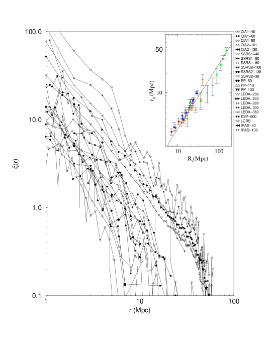
  Figure 2.  : Usual analysis based on the function $\xi(r)$ of the same galaxy catalogues of Fig.1. This analysis is based on the a priori and untested assumption of the analyticity and homogeneity. These properties are not present in the real galaxy distributions and the results appear therefore rather confusing. This lead to the impression that galaxy catalogues are not good enough and to a variety of theoretical problems like the galaxy cluster mismatch, luminosity segregation, the linear and non linear evolution, etc.. The situation changes completely and it becomes rather clear if one adopts the more general framework that is at the basis of Fig.1. In the insert panel we show the dependence of $r_{0}$ on $R_{s}$ for all the catalogs. The linear behaviour is a consequence of the fractal nature of galaxy distribution in these samples.

• A possible explanation of the shift of $r_{0}$ is based on the luminosity segregation effect [Davis et al. (1988)] [Park et al. (1994)] [Benoist et al. (1996)]. The fact that the giant galaxies are more clustered than the dwarf ones, i.e. that they are located in the peaks of the density field, has given rise to the proposition that larger objects may correlate up to larger length scales and that the amplitude of the $\>\xi(r)$ is larger for giants than for dwarfs one. The deeper VL subsamples contain galaxies that are in average brighter than those in the VL subsamples with smaller depths. As the brighter galaxies should have a larger correlation length the shift of $r_{0}$ with sample size could be related, at least partially, with the phenomenon of luminosity segregation. The insert of Fig.2 show clearly the linear dependence of $r_{0}$ on $R_{s}$, which completely consistent with power law decay of $\Gamma(r)$. In this respect, the proposed luminosity bias effect appears essentially irrelevant.

References

- Benoist et al. (1996) Benoist C. et al.(1996) Astrophys. J., in print
- Coleman and Pietronero (1992) Coleman, P.H. and Pietronero, L., (1992) Phys.Rep. 231, pp.311-391
- Da Costa et al. (1994) Da Costa L.N., et al.(1994) Astrophys. J. 424 L1-L4
- Davis and Peebles (1983) Davis, M., Peebles, P. J. E. (1983) Astrophys. J. 267, 465-482
- Davis et al. (1988) Davis M. et al., (1988) Astrophys. J. 333, L9-L12
- Davis (1997) Davis M., (1997)(astro-ph/9610149) in the Proc. of the Conference ”Critical Dialogues in Cosmology” N. Turok ed.
- Mandelbrot (1982) Mandelbrot, B. (1982) The Fractal Geometry of Nature, Freeman, New York
- Montuori et al. (1997) Montuori M., Sylos Labini, F., Gabrielli, A., Amici A., Pietronero,L. (1997) Europhys. Lett. 39 103-108
- Montuori and Sylos Labini (1997) Montuori M. & Sylos Labini F.(1997) Astrophys. J. in print
- Park et al. (1994) Park, C., Vogeley, M.S., Geller, M., Huchra, J. (1994) Astrophys. J. 431 569
- Peebles (1993) Peebles, P.E.J., (1993) Principles of physical Cosmology Princeton Univ.Press.
- Sylos Labini (1994) Sylos Labini, F., (1994), Astrophys. J., 433, 464-467
- Sylos Labini et al. (1997) Sylos Labini, F., Montuori, M.and Pietronero, L. (1996), Phys. Rep. in print