Matter Mixing in Axisymmetric Supernova Explosion

Abstract

Growth of Rayleigh-Taylor (R-T) instabilities under the axisymmetric explosion are investigated by two-dimensional hydrodynamical calculations. The degree of the axisymmetric explosion and amplitude of the initial perturbation are varied parametrically to find the most favorable parameter for reproducing the observed line profile of heavy elements. It is found that spherical explosion can not produce $\rm{}^{56}Ni$ travelling at high velocity ($\sim 3000$km/sec), the presence of which is affirmed by the observation, even if the amplitude of initial perturbation is as large as $30\%$. On the other hand, strong axisymmetric explosion model produce high velocity $\rm{}^{56}Ni$ too much. Weak axisymmetric explosion are favored for the reproduction of the observed line profile. We believe this result shows upper limit of the degree of the axisymmetric explosion. This fact will be important for the simulation of the collapse-driven supernova including rotation, magnetic field, and axisymmetric neutrino radiation, which have a possibility to cause axisymmetric supernova explosion. In addition, the origin of such a large perturbation does not seem to be the structure of the progenitor but the dynamics of the core collapse explosion itself since small perturbation can not produce the high velocity element even if the axisymmetric explosion models are adopted.

Department of Physics, School of Science, University of Tokyo, 7-3-1 Hongo, Bunkyoku, Tokyo 113, Japan
The Institute of Physical and Chemical Research, Wako, Saitama, 351-01, JAPAN
Research Center for the Early Universe, Faculty of Science, University of Tokyo, 7-3-1 Hongo, Bunkyoku, Tokyo 113, Japan

1 Introduction

It is SN 1987A in Large Magellanic Cloud that provided us the apparent evidence of large-scale mixing in the ejecta for the first time. For example, the unexpected early detection of X-rays (Dotani et al (1987); Sunyaev et al (1987); Wilson et al (1988)) and gamma-rays (Matz et al (1988)) suggest the radioactive nuclei, which are synthesised at the bottom of the ejecta, are mixed up to the outer layer. The form of the X-ray light curve is also thought to be the indirect evidence of mixing and clumping of the heavy elements (e.g., Itoh et al (1987); Kumagai et al (1988)). Moreover, it is reported that a part of heavy elements, such as $\rm Fe_{II}$, $\rm Ni_{II}$, $\rm Ar_{II}$, and $\rm Co_{II}$, is mixed up to the fast moving ($\sim$3000-4000 km/s) outer layers from the observation of the width of its infrared spectral lines (Erickson et al (1988)). On the other hand, hydrogen which has the expansion velocity as low as 800 km/s is observed (H$\rm\ddot{o}$flich (1988)).

At present, the growth of R-T instability is thought to be the most promising mechanism for the explanation of the matter mixing. Although the idea that the instability grows during explosion in Type II supernova was not new (e.g., Falk & Arnett (1973); Chevalier (1976); Bandiera (1984)), there was necessity to calculate numerically the growth of the instability using realistic stellar models in multi-dimensions to see its effect quantitatively. With the improvement of the supercomputer, many people have done such calculations. Early two-dimensional simulations of the first few hours of the explosion showed that the R-T instabilities indeed grows (Arnett, Fryxell, & M$\rm\ddot{u}$ller (1989); Hachisu et al (1990); M$\rm\ddot{u}$ller, Fryxell, & Arnett (1990); Fryxell, Arnett, & M$\rm\ddot{u}$ller (1991); and M$\rm\ddot{u}$ller, Fryxell, & Arnett (1991)).

However, there are some points which are still open to arguments. For example, the location and amplitude of the seed of the R-T instability are still unknown. Up to the present, two candidates have been proposed for that seed. One is that the convection during the steady stellar evolution produces such seed. It is reported that the density fluctuation, $\delta\rho/\rho$, will be $\sim 5\%$ (up to $8\%$) at the beginning of the core collapse (Bazan & Arnett (1994); Bazan & Arnett (1997)) at the inner and outer boundaries of the convective O– rich shell, where the radioactive nuclei, such as $\rm{}^{56}Ni$, are mainly synthesised. The other is that core collapse will amplify the initial fluctuation in Fe core to the degree of $\delta R_{s}/R_{s}\sim 30\%$, where $R_{s}$ is shock radius (Burrows & Hayes (1995)).

Another problem is the reproduction of line profiles of heavy elements. The line profile of Co and Fe have shown that a small fraction of them is expanding at 3000-4000 km/s. On the other hand, numerical simulations can produce Co and Fe whose velocities are of order 2000 km/s at most even if the acceleration by the energy release of the radioactive nuclei is taken into account (Herant & Benz (1991); Herant & Benz (1992)). Although they insist that pre-mixing of $\rm{}^{56}Ni$ will be necessary for the reproduction, the problem of the high velocity heavy elements seems to be unresolved.

There is another approach to that solution. If the explosion itself is not spherical symmetry, the situation will change dramatically. There are some reasons we should take account of the asymmetry in supernova explosion. Among them is a well-known fact that most massive stars are rapid rotators (Tassoul (1978)). It is well known that stars spin down as they evolve, especially through the red supergiant stage, meaning loss of their total angular momentums. However, pulsars which are found in supernova remnants are rotating rapidly, to be sure. This fact suggests that a large angular momentum is still in the center region of the star when it collapses. Since stars are rotating in reality, the effect of rotation should be investigated in numerical simulations of a collapse-driven supernova. Thus far, several simulations have been done by a few groups in order to study rotating core collapse (M$\rm\ddot{u}$ller, Rozyczka, & Hillebrandt (1980); Tohline, Schombert, & Boss (1980); M$\rm\ddot{u}$ller & Hillebrandt (1981); Bodenheimer & Woosley (1983); Symbalisty (1984); M$\rm\ddot{o}$nchmeyer $\&$ M$\rm\ddot{u}$ller (1989); Finn & Evans (1990); and Yamada & Sato (1994)). As a result, some numerical simulations of a collapse-driven supernova show the possibility of jet-like explosion if the effect of a stellar rotation and/or stellar magnetic field is taken into consideration. There is also a possibility that the axisymmetrically modified neutrino radiation from a rotating proto-neutron star causes asymmetric explosion (Shimizu, Yamada, & Sato (1994)). We note these effects mentioned above tend to cause axisymmetric explosion. In addition, axisymmetric explosion has an advantage to the explanation of some observational facts. For example, it is reported that axisymmetric explosion has a possibility to produce $\rm{}^{44}Ti$ so much as to explain the tail of the light curve of SN 1987A (Nagataki et al. (1997)). Furthermore, some observations of SN 1987A suggest the asymmetry of the explosion. The clearest is the speckle images of the expanding envelope with high angular resolution (Papaliolis et al. (1989)), where an oblate shape with an axis ratio of $\sim 1.2-1.5$ was shown. Similar results were also obtained from the measurement of the linear polarization of the scattered light from the envelope (Cropper et al. (1988)). If the envelope is spherically symmetric, there is no net linear polarization induced by scattering. Assuming again that the shape of the scattering surface is an oblate or prolate spheroid, one finds that the observed linear polarization corresponds to an axis ratio of $\sim 1.2$. We must note that the observed non-spherical nature of the morphology in the radio remnant of SN 1987A can be explained by the circumstellar medium inhomogeneities rather than explosion asymmetry (Gaensler et al. (1996)). However, this observation does not necessarily rule out the intrinsic asymmetric explosion. Because of these reasons mentioned above, it is important to investigate the effect of axisymmetric explosion on the mixing of the ejecta.

Based upon these facts, Yamada $\&$ Sato (Yamada & Sato (1991)) did two- dimensional hydrodynamical calculations under the axisymmetric and equatorial symmetric explosion. They found heavy elements could be highly accelerated in an axisymmetric explosion and get velocities of order of 4000km/s when the amplitude of the initial instabilities is as large as $\sim 30\%$.

However, their calculation has some points to be improved as mentioned below. At first, they calculate matter mixing only with one model, that is, the initial velocity behind the shock wave is assumed to be proportional to $r\times\cos^{2}\theta$, where $\theta$ is the zenith angle. This assumption is groundless and is not persuasive. Secondly, although they show the presence of the high velocity heavy elements in the calculation, they do not calculate line profiles of heavy elements, which should be compared with the observation. Thirdly, they assume that the chemical composition of the ejecta and the mass cut are spherically symmetric. Finally, since their numerical algorithm is Donner Cell method, we feel it necessary to make sure their results by more refined algorithm.

In this paper, the degree of the axisymmetric explosion is changed parametrically and the velocity distribution of heavy nuclei is calculated for each model. We will make a limit to the degree of the axisymmetric explosion and the initial fluctuation by comparing the results with observations. In each calculation, the results of explosive nucleosynthesis under its explosion are used for the chemical composition and mass cut (Nagataki et al. (1997)). Moreover, Roe’s scheme of second-order accuracy in space (Hirsch (1990); Shimizu (1995); Shimizu (1996)) is adopted for the calculation.

We show our method of calculation for the matter mixing in section 2. Results are presented in section 3. Summary and discussion are given in section 4.

2 Model and Calculations

2.1 Hydrodynamics

We performed two-dimensional hydrodynamical calculations. The calculated region corresponds to a quarter part of the meridian plane under the assumption of axisymmetry and equatorial symmetry. The number of meshes is $2000\times 100$ (2000 in the radial direction, and 100 in the angular direction). The size of radial meshes is arranged so as to increase like geometrical series. Both of the inner most radius and mesh size are set to be $10^{8}\rm cm$. The outer most radius is set to be $3.3\times 10^{12}\rm cm$, that is, the surface of the progenitor. As for the algorithm, we use the Roe’s scheme of a second-order accuracy in space. The basic equations are as follows:

$$\partial_{t}\rho= -\frac{1}{r^{2}}\partial_{r}(\rho u_{r}r^{2})-\frac{1}{r\sin\theta}\partial_{\theta}(\rho u_{\theta}\sin\theta),$$

$$\partial_{t}(\rho u_{r})= -\frac{1}{r^{2}}\partial_{r}(\rho u_{r}^{2}r^{2})-\frac{1}{r\sin\theta}\partial_{\theta}(\rho u_{r}u_{\theta}\sin\theta)$$

$$-\partial_{r}P+\frac{\rho u_{\theta}^{2}}{r},$$

$$\partial_{t}(\rho u_{\theta})= -\frac{1}{r^{2}}\partial_{r}(\rho u_{\theta}u_{r}r^{2})-\frac{1}{r\sin\theta}\partial_{\theta}(\rho u_{\theta}^{2}\sin\theta)$$

$$-\frac{1}{r}\partial_{\theta}P-\frac{\rho u_{\theta}u_{r}}{r},$$

$$\partial_{t}E= -\frac{1}{r^{2}}\partial_{r}\left[(E+P)u_{r}r^{2}\right]$$

$$-\frac{1}{\sin\theta}\partial_{\theta}\left[(E+P)u_{\theta}\sin\theta\right]$$

where $\rho,P,$ and $E$ are the mass density, pressure, total energy density per unit volume and $u_{r}$ and $u_{\theta}$ are velocities of a fluid in $r$ and $\theta$ direction, respectively. The first equation is the continuity equation, the second and third are the Euler equations and the forth is the equation of the energy conservation. We use the equation of state:

$$P=\frac{1}{3}aT^{4}+\frac{\rho k_{B}T}{A_{\mu}m_{u}}$$

where $a$, $k_{B}$, $A_{\mu}$ and $m_{u}$ are the radiation constant, Boltzmann constant, the mean atomic weight, and the atomic mass unit, respectively.

In this paper, We assume the system is adiabatic after the passage of the shock wave, because the entropy produced during the explosive nucleosynthesis is much smaller than that generated by the shock wave. This means the effect of nickel bubble is not included in this study.

2.2 Post-processing

In order to see how the matter is mixed by R-T instabilities quantitatively, we use a test particle approximation. We will explain this approximation.

At first, test particles are put in the progenitor. It is assumed that test particles are at rest and scattered in the Si– rich and inner O– rich layers, where heavy radioactive elements are mainly synthesised by the explosive nucleosynthesis, with the same interval in the radial and angular directions in each layer. We put $(10(r)\times 100(\theta))$ particles in each layer. Additionally, we also put $(10(r)\times 100(\theta))$ particles in outer O–, He–, and H– rich layers in the same way. The initial positions of test particles are summarized in Table 1.

In calculating the degree of the mixing, we assume that each test particle has its own mass which is determined by the initial distribution of the test particles so that their sum becomes the mass of the Si–, O–, He–, and H– rich layers, and also assume that each test particle has its own composition which is determined by the calculation of explosive nucleosynthesis. We use the results of Nagataki et al. (1997) (hereafter NHSY) for the composition as stated below.

As mentioned above, it is assumed that test particles are at rest at the beginning (t=0). We also assume that they move with the local velocity at their positions after the passage of a shock wave. Thus we can calculate each particle’s path by integrating $\displaystyle{\partial\vec{x}/\partial t}=\vec{v}(t,\vec{x})$, where the local velocity $\vec{v}(t,\vec{x})$ is given from the hydrodynamical calculations. In this way, we can calculate the degree of the mixing quantitatively and can calculate the velocity distribution of each element, such as $\rm{}^{56}Ni$ at each time.

2.3 Hydrodynamical initial condition

At first, we will explain the initial shock wave. Since there is still uncertainty as to the mechanism of Type II supernova, all calculations of matter mixing have not been performed from the beginning of the core collapse. Instead, explosion energy is deposited artificially at the innermost boundary (e.g., Hachicu et al (1992)). In this paper, this method is taken and the explosion energy of $1.0\times 10^{51}\rm erg$ is injected to the region from $1.0\times 10^{8}\rm cm$ to $1.5\times 10^{8}\rm cm$ (that is, at the Fe/Si interface).

As for the axisymmetric explosion, In this paper, the initial velocity of matter behind the shock wave is assumed to be radial and proportional to $r\times[1+\alpha\cos(2\theta)]/[1+\alpha]$, where r, $\theta$, and $\alpha$ are the radius, the zenith angle, and the free parameter which determine the degree of the axisymmetric explosion, respectively. Since the ratio of the velocity in the polar region to that in the equatorial region is 1 : $(1-\alpha)/(1+\alpha)$, more extreme jet-like shock waves are obtained as the $\alpha$ gets larger. In the present study, we take $\alpha=0$ for the spherical explosion and $\alpha=1/3,\;3/5,\;\rm and\;7/9$ (these values mean that the ratios of the velocity are 2:1, 4:1, and 8:1, respectively) for the axisymmetric ones (see Table 2). We assumed that the distribution of thermal energy is same as the velocity distribution and that the total thermal energy is equal to the total kinetic energy.

Next, in order to see the evolution of the fluctuation, we must introduce perturbation artificially. From the linear stability analysis, the linear growth rate is given as (Chankrasekhar (1981))

$$G^{2}_{RT}=\frac{\rho_{+}-\rho_{-}}{\rho_{+}+\rho_{-}}kg_{eff}$$

where $\rho_{+}$, $\rho_{-}$, $k$, and $g_{eff}$ are the densities in the upper and lower layers, the wavenumber of the density perturbation, and effective gravity, respectively. In our calculation, the effective gravity is nearly equal to $-dP/\rho dr$.

As one can see from the growth rate, perturbations of shorter wavelengths grow faster than that of longer ones. So it is very important information what the power spectrum of density perturbation of a star is. However, this power spectrum has not been known from observations. Only some numerical simulations of the progenitor predict the spectrum (Bazan & Arnett (1994); Bazan & Arnett (1997)). Moreover, numerical calculations inherently introduces some amount of viscosity that suppresses the growth of instabilities of wavelength shorter than a certain value, which will grow at fastest rate if such perturbations exist actually. We must keep in mind that numerical calculations of R-T instabilities in a star have uncertainty mentioned above.

Historically speaking, there are two ways of introducing perturbations. One is periodic method and the other is random perturbation method. In the periodic perturbation method, a growing mode is given $a$ $priori$ and characteristic wavelength is not given in the random perturbation method. Anyway, their methods assume a form of power spectrum and there is no guarantee that a real star has such a form.

In this paper, we took a periodic perturbation method since we consider it better rather than random perturbations since we are interested in the different growth rate in different direction (Yamada & Sato (1991)) under the same fluctuation pattern. As many people have done, we perturb only velocity field inside the shock wave when the shock front reaches the He/H interface. When we calculate the axisymmetric explosion, we introduce perturbation when the shock front in polar region reaches that interface. We adopt monochromatic perturbations, i.e., $\delta v\;=\;\varepsilon v(r,\theta)\cos(m\theta)$ (m=20). In this paper, we performed calculations with three values of perturbations, that is, $0\%$, $5\%$, and $30\%$ were taken for the value of $\varepsilon$. These model parameters are summarized in Table 3. We note that it is reported that mixing width, i.e. the length of the mushroom-like ’fingers’, depends on only slightly on the mesh resolution when $\varepsilon$ is larger than $\sim 5\%$ of the expansion speed (Hachicu et al (1992)). Because of this reason, we think that the influence of the power spectrum of the initial perturbation is relatively small in this study.

We note that the form of the initial shock wave and the degree of the initial fluctuation cannot be known directly from both observation and theory. Rather, we will attempt to make a limit to these initial conditions by comparing the results with the observations under the assumption of periodic perturbation.

2.4 Progenitor, Chemical composition, and Mass cut

The progenitor of SN 1987A, Sk-69^∘202, is thought to have had the mass $\sim 20M_{\odot}$ in the main-sequence stage (Shigeyama, Nomoto, & Hashimoto (1988); Woosley & Weaver (1988)) and had $\sim$ (6$\pm$1)$M_{\odot}$ helium core (Woosley (1988)). Thus, we use for the initial density of the progenitor the presupernova model which is obtained from the evolution of a helium core of 6 $M_{\odot}$ (Nomoto & Hashimoto (1988)), and their hydrogen envelope. Total mass of the progenitor corresponds to 16.3 $M_{\odot}$.

The chemical composition of the progenitor is changed by the nuclear burning when the shock wave passes (explosive nucleosynthesis). We used the results of NHSY for the explosive nucleosynthesis. For example, we show in Figure 1 the contour of mass fraction of $\rm{}^{56}Ni$ for S1 and A3 models. We note that this effect of the initial asymmetric chemical composition has never been considered in the previous studies.

As for the mass cut, we use the results of NHSY. We show in Figure 2 the mass cuts for S1 and A3 models. These mass cuts are chosen so as to contain 0.07$M_{\odot}$ $\rm{}^{56}Ni$ in the ejecta. However, we must note that defining the form of the mass cut is very difficult problem since it is sensitive not only to the explosion mechanism, but also to the presupernova structure, stellar mass, and metallicity (Woosley & Weaver (1995)). Moreover, the form of the mass cut has a large influence on the mixing of $\rm{}^{56}Ni$ since it is mainly produced near the mass cut. Because of these reasons, we must investigate the sensitivity of the results on the mass cut as seen in section 3.2.

3 Results

3.1 Global density structure and Position of $\rm{}^{56}Ni$

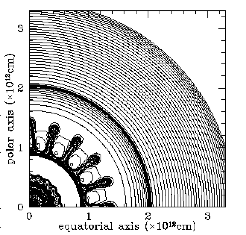
Figure 3: Density contour for S1b model at t = 5000 sec. The shock wave can be seen at the radius $\sim 2\times 10^{12}$ cm. The growth of R-T instabilities can be seen inside the shock wave.

In this paper, 12 models are performed in all. We show the density contours of S1b at time = 5000 sec in Figure 3. Mushroom-like ’fingers’, which are characteristic of the nonlinear growth of Rayleigh-Taylor instability, can be seen in this model. This is consistent with the work done by other groups (e.g., Fryxell, Arnett, & M$\rm\ddot{u}$ller (1991); Hachicu et al (1992)). From this point of view, we think that the resolution of our calculations are high enough to see the global behavior of the matter mixing.

Next, positions of test particles are shown at time = 5000 sec for S1b and S1c in Figure 4. For comparison, we show those for A3b and A3c in Figure 5. As expected, the matter is mixed more in the larger initial perturbation model (S1c and A3c models). We can also see that the matter is mixed more in the polar region than in the equatorial region for the axisymmetric explosion model (A3b and A3c models).

Before we go to the next subsection, we must comment on the effect of two-dimensional calculations. All calculations presented here are performed in two dimensions so as to save our computer’s CPU-time and memory and to allow the extensive exploration of the parameter space carried out in this study. Readers should note here that there is a tendency that three-dimensional modes grow to higher mixing velocities than two-dimensional modes (Remington et al (1991); Yabe (1991); Marinak et al (1995)). This seems to be the reason why the finger at the $\theta=0^{\circ}$ axis is further along than at $\theta=90^{\circ}$ axis even if the spherical explosion model of S1c. However, three-dimensional simulations of the explosion of SN 1987A (M$\rm\ddot{u}$ller, Fryxell, & Arnett (1990)) have shown little change in relation to the two dimensional case. Moreover, by comparing figure 4 with figure 5, we think that the effect of axisymmetric explosion is quite large compared with the two-dimensional effect. It is true that the three-dimensional effect should be investigated with high resolution in the future, but we think our quantitative estimates discussed below are not unreasonable.

3.2 Velocity distribution of $\rm{}^{56}Ni$

We will pay attention to $\rm{}^{56}Ni$, which is responsible for the behavior of the bolometric light curve, the early detection of X-yay and Gamma-ray, and their light curves.

At first, we will make investigation into the velocity distributions of $\rm{}^{56}Ni$ for all models. Figure 6 and Figure 7 are the results of them. We can see that the range of velocity gets wider as the initial perturbation gets larger for any explosion model, that is, irrespective of the value of $\alpha$. However, high velocity $\rm{}^{56}Ni$ of order 3000-4000 km/sec can not be produced in the spherical explosion case even if the initial perturbation is as large as 30$\%$. On the other hand, such high velocity $\rm{}^{56}Ni$ is produced for any axisymmetric explosion for the case of 30$\%$ initial perturbation. However, high velocity $\rm{}^{56}Ni$ seems to be produced too much for strong axisymmetric explosion case (see A2c and A3c model in Figure 7). This might be a constraint for the degree of axisymmetric explosion. We will investigate this suggestion more carefully in the following.

Before we go to the further discussion, we make a comment on the average velocity of $\rm{}^{56}Ni$. In the perturbed models, slower velocity component and higher velocity component appear naturally compared with no perturbed models since the way of perturbation is monochromatic. As $\epsilon$ becomes large, its degree also becomes large. In fact, it can be seen in Figure 4, 5 that the radius of inner most layer is smaller in the $30\%$ models compared with $5\%$ models. At the same time, the mixing width is larger in the $30\%$ models. In other words, it seems that the ram pressure due to ingoing bubbles of lighter elements suppressed the bulk velocity of heavy elements while a part of them are accelerated by the outgoing mushrooms. The average velocity of $\rm{}^{56}Ni$ is determined how much $\rm{}^{56}Ni$ is taken in the mushroom and how much $\rm{}^{56}Ni$ is remained in the inner most region. As a consequence, the average velocity of $\rm{}^{56}Ni$ does not necessarily gets higher together with $\epsilon$. In fact, we can see in Figure 6 that the average velocity of $\rm{}^{56}Ni$ becomes lower in the $5\%$ models compared with no perturbed models.

Next, we calculate line profiles for optically thin ejecta and compare them with observations to examine the suggestion mentioned above. However, interpretation of calculated line profiles is complicated by the line of sight of the observer. The symmetry axis inferred from the observation of the ring of SN 1987A (Plait et al. (1995)) is different from that inferred from the speckle interferometry (Papaliolis et al. (1989)). In this paper, we calculate line profiles seen from $\theta=44^{\circ}$, which is inferred from the ring of SN 1987A. The results are shown in Figure 8 and  9. For comparison, observed infrared line profiles of Fe from SN 1987A is shown in Figure 10. As for the spherical explosion, high velocity element can not be seen. On the other side, as $\alpha$ gets large, the form of line profile becomes to be different from that of observations. In particular, it is unlikely that the strong axisymmetric explosion model ($\alpha=3/5,7/9$ case) can reproduce the line profile. We can say that the model A1c most closely resembles the line profile including high velocity element.

Finally, as mentioned in section 2.4, we must examine the sensitivity of our results on the mass cut. We can easily guess that the small velocity element will get larger if the mass cut is assumed to be spherical since the velocity is small near the equatorial region, which is cut by the axisymmetric mass cut. We show line profiles incorporating the spherical mass cut for comparison in Figure 11 and  12. As we expected, the figure shows the enhancement of small velocity element. However, A2c and A3c model are still far from the observed line profile. From this result, we think A2 and A3 model are rejected by the observation. On the other hand, model A1c begins to resemble to the observations. This supports the proposal that model A1c can reasonably reproduce the observation. We also performed a simulation in order to investigate the effect of asymmetric explosive nucleosynthesis (Nagataki et al. (1997)) on the velocity distribution of $\rm{}^{56}Ni$. It is found, however, that the effect of asymmetric mass cut is of much more importance.

3.3 Minimum velocity of hydrogen

Additionally, we see the minimum velocity of hydrogen. The results are summarized in Table 4. We can identify the tendency for the minimum velocity to become lower as the degree of axisymmetric explosion gets larger when the initial perturbation is set to be zero. It is also seen that as the initial perturbation amplitude is increased, the minimum velocity decreases for the same degree of the axisymmetric explosion. However, we can not say that the minimum velocity decreases as the degree of axisymmetric explosion and initial perturbation are both increased. Although we can not explain the reason clearly, we can only say that all models which have an initial perturbation larger than $5\%$, can explain the observation, which shows the minimum velocity of hydrogen $\sim 800$ km/sec.

4 Summary and Discussion

We have performed a two-dimensional hydrodynamic calculation for an axisymmetric explosion with a periodic perturbation. The degree of the explosion axisymmetry is varied and three perturbation amplitudes are studied for each explosion. We have compared calculated line profiles to observations, with special attention paid to the high velocity element. Limits on initial perturbation amplitude and degree of axisymmetry are established based on our comparison.

We find the high velocity element can not be produced for any spherical explosion model even if the initial perturbation amplitude is as large as $30\%$. On the other hand, it is produced by the axisymmetric explosion, if the initial perturbation amplitude is $30\%$. As for the origin of the perturbation, we cannot attribute such a large perturbation ($\sim 30\%$) to the structure of the progenitor (Bazan & Arnett (1994); Bazan & Arnett (1997)). We feel that only the dynamics of the core-collapse explosion itself can lead such a large perturbation. However, we must note that if other mechanisms, such as nickel bubbles, works effectively, the amplitude to be desired will be less than $30\%$. We also add a comment on another possible source of a large perturbation. It is the offset of the core from the center of mass of the star. This is being studied now by Peter Goldreich as the effect of gravity waves from convective zones acting in constructive interference as they converge towards the core. This leads to some oscillatory behavior of the core about the center of mass. However, the amplitude of its perturbation generated by its effect is not reported yet.

The line profiles also serve as upper limits on the degree of explosion axisymmetry. Line profiles are affected by the presence of a mass cut. However, models of A2c and A3c can not reproduce the observed line profile even if different mass cut positions are incorporated. We think this provides an upper limit of the degree of the axisymmetric explosion. This fact will be important for the simulation of the collapse-driven supernova including rotation, magnetic field, and axisymmetric neutrino radiation.

On the other hand, the weak axisymmetric model, A1c best reproduces the observations, including the high velocity element. Since the line profile is also changed by the angle between our line of sight and polar axis and radiative transfer, the information provided by the line profile is ambiguous. We can only say that there is an axisymmetric explosion model that can reproduce the line profile.

To provide an additional constraint, we calculated the lowest velocity of hydrogen. The results showed that any explosion model can explain the observed value $\sim 800$km/sec if the amplitude of the initial perturbation is larger $5\%$.

We must note that our results are obtained on the assumption of periodic perturbation method. As stated in subsection 2.3, the effect of initial power spectrum of density perturbations should be explored in future. In particular, it will be important to perform R-T calculations using the asymmetric progenitor models (Bazan & Arnett (1994); Bazan & Arnett (1997)) since their two-dimensional models predict the power spectrum of density perturbations. Their models may also have a key for the reproduction of the observed line asymmetry like that in Figure 10. However, we think that the influence of the power spectrum of the initial perturbation is relatively small in this study since the amplitudes of initial perturbations are larger than $5\%$ of the expansion speed (Hachicu et al (1992)).

We also make a comment on the effect of Coriorlis force. When instabilities of other targets that have enough angular velocity, such as an accretion disk around a black hole, are explored (Ruffert $\&$ Arnett (1994)), Coriorlis force will play an important role with respect to the growth of instabilities. However, we neglected the rotation of the mantle and envelope in this paper since the rotation velocity is much smaller than the explosion velocity where the R-T instabilities grow.

We will consider the reliability of our calculations. Grid resolution is relevant since higher resolution can better reproduce the steep gradient of physical quantities, such as those for density, pressure, and temperature. Fryxell, M$\rm\ddot{u}$ller, and Arnett have shown that the minimum resolution required for a ’converged’ model is determined by the hydrodynamic algorithm and that there is a possibility that numerical errors might dominate the physical instability in much work which has already been done. On the other hand, Hachisu et al have shown the mixing width is insensitive to resolution in their Roe’s third order TVD scheme if the initial amplitude of the velocity perturbation is larger than $1\%$ of the local sound speed (Hachicu et al (1992)). It is important to see the structure of the mushrooms in detail, to be sure, but our main purpose is to see the global behavior of the material. We think our calculations have enough resolution for that purpose. For example, we can see the mushroom-like ’Finger’ in the S1b case. Since the finger cannot be seen clearly in Yamada & Sato (1991) under the same condition but can be seen in other groups (e.g., Hachicu et al (1992)), we conclude that our method is an improvement to that in Yamada & Sato (1991) and that our axisymmetric explosion models employ sufficient resolution to accurately describe the global behavior of the material.

Figure 1: Left: Contaur of the mass fraction of ${}^{56}\rm Ni$ in the S1 model. The maximum value of the mass fraction of${}^{56}\rm Ni$ is 9.3$\times 10^{-1}$. The region where mass fraction of ${}^{56}\rm Ni$ becomes 0.9 is noted in the figure. Right : Same as left but for A3 model. The maximum value is 9.1$\times 10^{-1}$. Contours are drawn for the initial position of test particles.

Figure 2: Form of the mass cut for S1 case and A3 case. Dots are plotted for the initial positions of the test particles which will be ejected.

Figure 4: Positions of test particles at time = 5000 sec after explosion. Left: S1b model. Right: S1c model.

Figure 5: Same as Fig.4 but for A3b and A3c models.

Figure 6: Velocity distribution of $\rm{}^{56}Ni$ at time = 5000 sec after explosion. Left: S1 model. Right: A1 model.

Figure 7: Same as Fig.6 but for A2 and A3 model.

Figure 8: Line profile of $\rm{}^{56}Ni$ seen from $\theta=44^{\circ}$ at time = 5000 sec after explosion. Left: S1 model. Right: A1 model.

Figure 9: Same as Fig.8 but for A2 and A3 model.

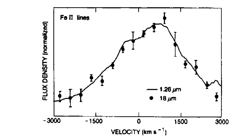
Figure 10: Observed infrared line profiles for Fe at 1.26 $\mu m$ (solid line, t = 377 days: Spyromilio et al. 1990) and at 18 $\mu m$ (data points, t = 407 days; Haas et al. 1990). Positive velocities (km/sec) correspond to a redshift.

Figure 11: Line profile of $\rm{}^{56}Ni$ for A1 model seen from $\theta=44^{\circ}$ at time = 5000 sec after explosion under the spherical mass cut.

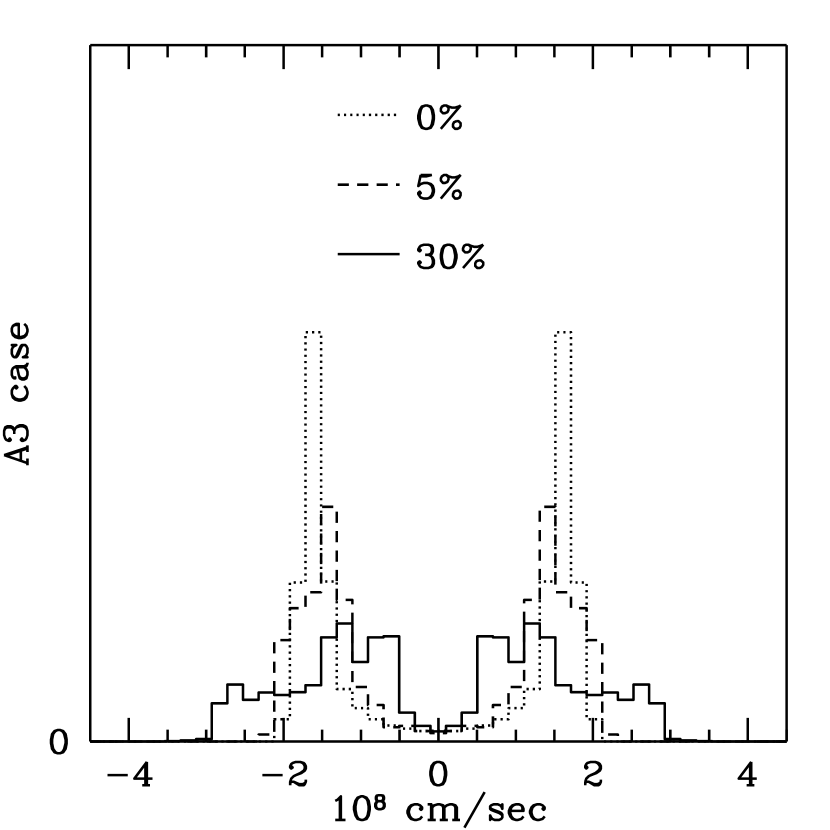
Figure 12: Same as Fig.11 but for A2 and A3 model.

Table 1: Initial positions of test particles

radius [cm]	number
$(1.5-3.0)\times 10^{8}$	1000
$(3.0-9.0)\times 10^{8}$	1000
$9.0\times 10^{8}-6.3\times 10^{9}$	1000
$6.3\times 10^{9}-4.8\times 10^{10}$	1000
$4.8\times 10^{10}-3.3\times 10^{12}$	1000

Model	S1	A1	A2	A3
$\alpha$	0	1/3	3/5	7/9
$V_{p}$:$V_{e}$	1:1	2:1	4:1	8:1

Table 2: Models for the initial shock wave. The first row shows names for each model. Second is the value of $\alpha$ for each model. Third is the ratio of the velocity in the polar region ($\theta=0^{\circ}$) to that in the equatorial region ($\theta=90^{\circ}$).

Model	$\alpha$	Perturbation[$\%$]	Model	$\alpha$	Perturbation[$\%$]
S1a	0	$0$	A2a	3/5	0
S1b	0	$5$	A2b	3/5	5
S1c	0	$30$	A2c	3/5	30
A1a	1/3	$0$	A3a	7/9	0
A1b	1/3	$5$	A3b	7/9	5
A1c	1/3	$30$	A3c	7/9	30

Table 3: Name of each model, the value of $\alpha$, and the amplitude of the initial perturbation.

	S1	A1	A2	A3
a	1.6	1.5	1.3	1.1
b	0.87	0.89	0.86	0.90
c	0.85	0.53	0.57	0.76

Table 4: Minimum velocity of hydrogen at time = 5000 sec. The unit is $10^{8}$cm/sec. ’a’ denotes that the amplitude of initial perturbation = 0$\%$. ’b’ and ’c’ denote $5\%$ and $30\%$, respectively.

References

- Arnett, Fryxell, & Mller (1989) Arnett, W.D., Fryxell, B.A., and Muller, E. 1989, ApJ, 341, L63
- Bandiera (1984) Bandiera, R. 1984, A&A, 139, 368
- Bazan & Arnett (1994) Bazan, G., and Arnett, W.D. 1994, ApJ, 433, L41
- Bazan & Arnett (1997) Bazan, G., and Arnett, W.D. 1997, astro-ph/9702239
- Bodenheimer & Woosley (1983) Bodenheimer, P., Woosley, S.E. 1983, ApJ, 269, 281
- Burrows & Hayes (1995) Burrows, A., and Hayes, J. 1995, ApJ, 450, 830
- Chankrasekhar (1981) Chandrasekhar, S. 1981, Hydrodynamic and Hydromagnetic Stability (New York:Dover)
- Chevalier (1976) Chevalier, R.A. 1976, ApJ, 207, 872
- Cropper et al. (1988) Cropper, M., Bailey, J., McCowage, J., Cannon, R.D., Couch, W.J., Walsh, J.R., Strade, J.O., and Freeman, F. 1988, MNRAS, 231, 695
- Dotani et al (1987) Dotani, T., et al 1987, Nature, 330, 230
- Erickson et al (1988) Erickson, E.F., Haas, M.R., Colgan, S.W.J., Lord, S.D., Burton, M.G., Wolf, J., Hollebach, D.J., and Werner, M. 1988, ApJ, 330, L39
- Falk & Arnett (1973) Falk, S.W., and Arnett, W.D. 1973, ApJ, 180, L65
- Finn & Evans (1990) Finn, L.S., Evans, C.R. 1990, ApJ, 351, 588
- Fryxell, Arnett, & Mller (1991) Fryxell, B., Arnett, W.D., and Mller, E. 1991, ApJ, 367, 619
- Gaensler et al. (1996) Gaensler, B. M., et al. 1997, ApJ, in press.
- Haas et al. (1990) Haas, R., Colgan, J., Erickson, F., Lord, D., Burton, G., and Hollenbach, J. 1990, ApJ, 360, 257
- Hachisu et al (1990) Hachisu, I., Matsuda, T., Nomoto, K., and Shigeyama, T. 1990, ApJ, 358, L57
- Hachicu et al (1992) Hachisu, I., Matsuda, T., Nomoto, K., and Shigeyama, T. 1992, ApJ, 390 230
- Herant & Benz (1991) Herant, M., and Benz, W. 1991, ApJ, 370, L81
- Herant & Benz (1992) Herant, M., and Benz, W. 1992, ApJ, 387, 294
- Hirsch (1990) Hirsch, C. 1990, Numerical Computation of Internal and External Flows, Volume 2 (John Wiley Sons, Chichester)
- Hflich (1988) Hflich, P. 1988, Proc. Astr. Soc. Australia, 7, 434
- Itoh et al (1987) Itoh, M., Kumagai, S., Shigeyama, T., Nomoto, K., and Nishimura, J. 1987, Nature, 330, 233
- Kumagai et al (1988) Kumagai, S., Itoh, M., Shigeyama, T., Nomoto, K., and Nishimura, J. 1988, A&A, 197, L7
- Marinak et al (1995) Marinak, M.M., et al. 1995, Phys. Rev. Lett, 75, 3677
- Matz et al (1988) Matz, S.M., Share, G.H., Leising, M. D., Chupp, E.L., Vestrand, W.T., Purcell, W.R., Strickman, M.S., and Reppin, C. 1988, Nature, 331, 416
- Mnchmeyer Mller (1989) Mnchmeyer, R.M., Mller, E. 1989 in NATO ASI Series, Timing Neutron Stars, p.549, ed.H.gelman E.P.J.van den Heuvel (New York:ASI)
- Mller, Rozyczka, & Hillebrandt (1980) Mller, E., Rozyczka, M., Hillebrandt, W. 1980, A&A, 81, 288
- Mller & Hillebrandt (1981) Mller, E., Hillebrandt, W. 1981, A&A, 103, 358
- Mller, Fryxell, & Arnett (1990) Mller, E., Fryxell, B.A., and Arnett, W.D. 1990, in The Chemical and Dynamical Evolution of Galaxies, ed. Ferrini, F., Matteucci, F., and Franco, J., (Pisa:Casa Editrice Giardini)
- Mller, Fryxell, & Arnett (1991) Mller, E., Fryxell, B.A., and Arnett, W.D. 1991, A&A, 251, 505
- Nagataki et al. (1997) Nagataki, S., Hashimoto, M., Sato, K., and Yamada, S. 1997, ApJ, 486, 1026.
- Nomoto & Hashimoto (1988) Nomoto, K., Hashimoto, M. 1988,Phys. Rep., 163, 13
- Papaliolis et al. (1989) Papaliolis, C., Karouska, M., Koechlin, L., Nisenson, P., Standley, C., Heathcote, S. 1989, Nature, 338, 13
- Plait et al. (1995) Plait, P., Lundqvist, P., Chevalier, R., and Kirshner, R. 1995, ApJ, 439, 730
- Remington et al (1991) Remington, et al, 1991, Phys. Rev. Lett, 67, 3259
- Ruffert Arnett (1994) Ruffert, M., Arnett, W. D. 1994, ApJ, 427, 351
- Shigeyama, Nomoto, & Hashimoto (1988) Shigeyama, T., Nomoto, K., Hashimoto, M. 1988, A&A, 196, 141
- Shimizu, Yamada, & Sato (1994) Shimizu, M.T., Yamada, S., Sato, K. 1994, ApJ, 432, L119
- Shimizu (1995) Shimizu, M.T. 1995, Ph.D.thesis, Univ. of Tokyo
- Shimizu (1996) Shimizu, M.T. 1996, RIKEN Review, 14, 27
- Spyromilio et al. (1990) Spyromilio, J., Meikle, S., and Allen, A. 1990, MNRAS, 242, 669
- Sunyaev et al (1987) Sunyaev, R.A. 1987, Nature, 330, 227
- Symbalisty (1984) Symbalisty, E.M.D. 1984, ApJ, 285, 729
- Tassoul (1978) Tassoul, J.L. 1978, Theory of Rotating stars (Princeton: Princeton Univ. Press)
- Tohline, Schombert, & Boss (1980) Tohline, J.E., Schombert, J.M., Boss, A.P. 1980 Space Sci. Rev., 27, 555
- Wilson et al (1988) Wilson, R.B., et al 1988, in Nuclear Spectroscopy of Astrophysical Sources, ed. Gehrels, N. and Share, G. (New York: AIP), p.66
- Woosley (1988) Woosley, S.E. 1988, ApJ, 330, 218
- Woosley & Weaver (1988) Woosley, S.E., Weaver, T.A. 1988, Phys. Rep., 163, 79
- Woosley & Weaver (1995) Woosley, S.E., Weaver, T.A. 1995, ApJS, 101, 181
- Yabe (1991) Yabe, T. 1991, Numer. Astrophys. Japan, 2, 247
- Yamada & Sato (1991) Yamada, S., Sato, K. 1991, ApJ, 382, 594
- Yamada & Sato (1994) Yamada, S., Sato, K. 1994, ApJ, 434, 268