Constraining cosmological models with cluster power spectra

Abstract

Using extensive $N$–body simulations we estimate redshift space power spectra of clusters of galaxies for different cosmological models (SCDM, TCDM, CHDM, $\Lambda$CDM, OCDM, BSI, $\tau$CDM) and compare the results with observational data for Abell–ACO clusters. Our mock samples of galaxy clusters have the same geometry and selection functions as the observational sample which contains 417 clusters of galaxies in a double cone of galactic latitude $|b|>30\hbox{${}^{\circ}$}$ up to a depth of 240 $h^{-1}{{\rm Mpc}}$.

The power spectrum has been estimated for wave numbers $k$ in the range $0.03\mathrel{\hbox{\hbox to0.0pt{\hbox{\lower 4.0pt\hbox{$\sim$}}\hss}\hbox{$<$}}}k\mathrel{\hbox{\hbox to0.0pt{\hbox{\lower 4.0pt\hbox{$\sim$}}\hss}\hbox{$<$}}}0.2\,\mbox{$h\,{{\rm Mpc}}^{-1}$}$. For $k>k_{{\rm max}}\simeq 0.05\,\mbox{$h\,{{\rm Mpc}}^{-1}$}$ the power spectrum of the Abell–ACO clusters has a power–law shape, $P(k)\propto k^{n}$, with $n\approx-1.9$, while it changes sharply to a positive slope at $k<k_{{\rm max}}$. By comparison with the mock catalogues SCDM, TCDM ($n=0.9$), and also OCDM with $\Omega_{0}=0.35$ are rejected. Better agreement with observation can be found for the $\Lambda$CDM model with $\Omega_{0}=0.35$ and $h=0.7$ and the CHDM model with two degenerate neutrinos and $\Omega_{{\rm HDM}}=0.2$ as well as for a CDM model with broken scale invariance (BSI) and the $\tau$CDM model. As for the peak in the Abell–ACO cluster power spectrum, we find that it does not represent a very unusual finding within the set of mock samples extracted from our simulations.

, , , , and

1 Introduction

It is widely believed that cosmic large–scale structures have been formed by gravitational instability from initially tiny Gaussian density perturbations, which result from quantum fluctuations at very early stages of cosmic evolution. The Standard Cold Dark Matter (SCDM) model is based on an inflationary model which predicts a scale–invariant spectrum of perturbations (the Harrison–Zeldovich spectrum) in an Einstein–de Sitter Universe. Most of the matter density in the Universe is provided by particles which interact only gravitationally and which were non–relativistic when the Universe became matter dominated. The nature of these dark matter particles is still unknown. Candidates for the cold dark matter particles are both the axions (light spin–0 bosons) and the lightest supersymmetric particles which have masses over 100 GeV, while massive neutrinos are candidates for hot dark matter particles.

However, the SCDM model is not compatible with existing observational data. Once suitably normalized to reproduce clustering features at scales of few Mpc, SCDM contradicts data at scales of few tens of Mpc, as well as the CMB anisotropies detected by the COBE satellite. This finding led to a large number of new theoretical models, the basic aim of which was to predict less power than the SCDM model on small scales, retaining, however, the enough power on the very large scales probed by COBE.

According to the standard picture of structure formation, the dark matter power spectrum $P(k)$ is expected to bend from its post–inflationary profile, and reaches a maximum at a wavenumber $k$ which depends on the parameters of the cosmological model. The corresponding length scale is of the order of a few 100 $h^{-1}{{\rm Mpc}}$. One of the major aims of current cosmological studies is to improve our knowledge of the structure of the Universe on scales which are between those probed by the best redshift surveys of galaxies and those probed by COBE.

Galaxy clusters are the largest gravitationally bound systems which we observe. They arise from high peaks of the initial density field (e.g., Bardeen et al. 1986) and have decoupled from the Hubble expansion relatively recently. Therefore, their properties and their spatial distribution are rather sensitive to the initial conditions for the development of gravitational instability. Large cluster samples include objects up to a depth of a few hundred Mpc and, to date, they cover much larger volumes than any available galaxy redshift survey. For this reason much effort has been devoted to compile large cluster samples, starting from the work by Abell (1958) and Abell, Corwin & Olowin (1989), and leading up to large redshift surveys both in the optical (e.g., Postman, Huchra & Geller 1992; Dalton et al. 1994; Collins et al. 1995) and in the X–ray (e.g., Nichol, Briel & Henry 1994; Romer et al. 1994; Ebeling et al. 1997). Employing X–ray selected as well as optically selected catalogues from machine based material is an attempt to overcome any subjective influence on the selection criteria that is possibly present in the Abell catalogue.

Historically, the analysis of the 2–point correlation function played an important role in analyzing large–scale structure. After having recognized the advantages of direct power spectrum estimation, this method has been developed as a standard tool in cosmology. Nowadays, much valuable information about structure formation is gained from power spectra of galaxies in redshift surveys (e.g., Feldman, Kaiser & Peacock 1994; Park et al. 1994; Lin et al. 1996; Schuecker, Ott & Seitter 1996; Tadros & Efstathiou 1996; cf. also Strauss & Willick 1995, and references therein).

Starting from the pioneering papers of Bahcall & Soneira (1983) and Klypin & Kopylov (1983), who estimated the 2–point cluster correlation function, galaxy clusters have been widely used for the determination of parameters of large–scale structure. The power spectrum of Abell clusters was calculated firstly by Peacock & West (1992), and, independently, by Einasto et al. (1993) and Jing & Valdarnini (1993). Einasto et al. (1997a) have determined the cluster power spectrum by inverting the 2–point correlation function of the cluster redshift compilation by Andernach et al. (1995).

In this paper we compare the clustering properties of a redshift catalogue of Abell–ACO clusters defined by Borgani et al. (1995) (cf. also Plionis & Valdarnini 1991) with that of mock cluster samples extracted from a set of $N$–body simulations of seven cosmological models. Recently the same catalogue of Abell–ACO clusters has been used to derive the Minkowski functionals (Kerscher et. al. 1997) of the cluster distribution and to compare it with that of mock samples from simulations.

This paper is organized as follows. In Sect. 2 we introduce briefly the cosmological models which we intend to discuss. In Sect. 3 we describe the observational sample and the construction of mock samples from numerical simulations. In Sect. 4 (and in a more technical appendix) we describe the analysis of the cluster power spectrum. In Sect. 5 we present and discuss our results. We summarize and draw the main conclusions in Sect. 6.

2 Cosmological models and numerical simulations

Besides the SCDM model we consider six other models, which are described in Table 1. We used the transfer function by Bardeen et al. (1986) and normalized the linear DM power spectra according to either the two year COBE data (Bennett et al. 1994, B94) or the four year COBE data (Górski et al. 1996, G96; Górski et al. 1998, G98). The $\tau$CDM model is normalized to the observed cluster abundance (Viana & Liddle 1996, V96). We have checked that a 20% change in the normalization does not change the power spectrum of the galaxy clusters selected from the simulations once the number of clusters is fixed. In particular, for a given model the result did not depend on the COBE normalization chosen (first, second, or fourth year). This confirms earlier results by Croft & Efstathiou (1994) and Borgani et al. (1995). For this reason, we also did not take into account any possible gravitational wave contribution, which would reduce the BSI and TCDM normalizations. We also did not take into account any correction to the power spectrum shape due to a non–negligible baryon fraction.

The SCDM model with Harrison–Zeldovich primordial spectrum (as predicted by the simplest inflationary models) assumes $\Omega_{0}=1$ and $h=0.5$. We consider it here as a reference model which, however, is generally accepted to be ruled out, since it has a too shallow power spectrum shape on intermediate scales ($10-50\,\mbox{$h^{-1}{{\rm Mpc}}$}$), and too much power on small scales ($<10\,\mbox{$h^{-1}{{\rm Mpc}}$}$) once normalized to the detected level of CMB anisotropy.

An exponential inflaton potential leads to power law inflation and, consequently, to a scale–free tilted (TCDM) model (e.g., Lucchin & Matarrese 1985). We assume here a spectral index $n=0.9$ after inflation. As the result of the tilt the TCDM model with $h=0.5$ has a lower normalization than SCDM in terms of the r. m. s. mass fluctuation $\sigma_{8}$.

The CHDM model assumes a mixture of cold and hot dark matter. The 20% contribution of the hot component is assumed to be shared between two neutrinos of equal mass (Primack et al. 1995).

Lowering the matter content ($\Omega_{0}<1$) shifts the maximum of the fluctuation spectrum to larger scales and steepens the spectrum on scales $\mathrel{\hbox{\hbox to0.0pt{\hbox{\lower 4.0pt\hbox{$\sim$}}\hss}\hbox{$<$}}}50\,\mbox{$h^{-1}{{\rm Mpc}}$}$. In the $\Lambda$CDM model a cosmological constant $\Omega_{\Lambda}\equiv\Lambda/(3H_{0}^{2})=1-\Omega_{0}$ makes the spatial curvature of the Universe negligible, as expected from standard inflationary models. Our $\Lambda$CDM model assumes $h=0.7$, a cosmological constant equivalent to $\Omega_{\Lambda}=0.65$.

The Open–bubble inflation model proposed by Ratra and Peebles (1994) and the open model with scale–invariant spectrum (Wilson 1983) are reasonably consistent with current observational data if $0.3\mathrel{\hbox{\hbox to0.0pt{\hbox{\lower 4.0pt\hbox{$\sim$}}\hss}\hbox{$<$}}}\Omega_{0}\mathrel{\hbox{\hbox to0.0pt{\hbox{\lower 4.0pt\hbox{$\sim$}}\hss}\hbox{$<$}}}0.6$ (Górski et al. 1998). We investigated the Open–bubble inflation CDM (OCDM) model with $h=0.65$, $\Omega_{0}=0.35$ and the normalization by G98.

The Broken Scale Invariant (BSI) cosmological model is specified by two parameters, the step location at $k_{\rm{break}}^{-1}=1.5\,\mbox{$h^{-1}{{\rm Mpc}}$}$ and its relative height $\Delta=3$; the normalization is $\sigma_{8}=0.60$. These parameters are related to the initial energy densities and mass ratios of the inflaton fields in the underlying inflationary model (Gottlöber, Müller & Starobinsky 1991, Gottlöber 1996). The original choice for such parameters has been based on the linear–theory comparison with different observational constraints (Gottlöber, Mücket & Starobinsky 1994). Analysis based on $N$–body simulations have been discussed by Amendola et al. (1995), Kates et al. (1995) and Ghigna et al. (1996). Recently, Lesgourgues et al. (1997) have discussed a BSI spectrum in a model with cosmological constant.

The $\tau$CDM model, which assumes a decaying massive $\tau$ neutrino as the dark matter constituent, has been originally proposed by Efstathiou et al. (1992a; see also White et al. 1995). Similarly to the BSI model, the $\tau$CDM model is characterized by two additional free parameters, namely the mass and the life time of the decaying massive particle, which are related to the scale where the spectrum changes and the amount of small–scale power suppression relative to the SCDM case. We consider the CDM model with a shape parameter of $\Gamma=0.21$ as a representation of the $\tau$CDM model (Jenkins et al. 1998). Normalized to the observed abundance of clusters (V96) this spectrum is very similar to the COBE normalized BSI spectrum.

Table 1: The model parameters. Column 2: the density parameter $\Omega_{0}$; Column 3: the Hubble parameter $h$; Column 4: the COBE predicted linear r. m. s. fluctuation amplitude at $8\mbox{$h^{-1}{{\rm Mpc}}$}$ $\sigma_{8}$; Column 5: reference to the normalization, Column 6: further model parameters

Model	$\Omega_{0}$	$h$	$\sigma_{8}$	normalization	model parameters
SCDM	1.0	0.50	1.37	B94
TCDM	1.0	0.50	1.25	B94	$n$ = 0.9
CHDM	1.0	0.50	0.67	G96	$\Omega_{{\rm HDM}}=0.2$, 2$\nu$
$\Lambda$CDM	0.35	0.70	1.30	B94	$\Omega_{\Lambda}=0.65$
BSI	1.0	0.50	0.60	B94	$k_{\rm{break}}^{-1}=1.5\,\mbox{$h^{-1}{{\rm Mpc}}$}$, $\Delta=3$
$\tau$CDM	1.0	0.50	0.60	V96	$\Gamma=0.21$
OCDM	0.4	0.65	0.58	G98

We evolve the initial density field starting from redshift $z=25$ ($z=30$ for CHDM) until the present epoch, by employing a PM $N$–body code with $300^{3}$ particles of mass $m_{{\rm p}}=1.3\times 10^{12}\,h^{-1}\Omega_{0}{{\rm M_{\hbox{$\odot$}}}}$. Cold particles in the CHDM simulations have a mass which is 20% smaller than this value. The simulation used $600^{3}$ grid cells in a simulation box of $L=500\,\mbox{$h^{-1}{{\rm Mpc}}$}$ comoving length a side. This provides a formal spatial resolution of less than $1\,\mbox{$h^{-1}{{\rm Mpc}}$}$. The simulation box is large enough to contain all fluctuation modes which contribute to the large–scale cluster distribution at the scales we are interested in. In order to account for the effect of cosmic variance, we carried out simulations for several random realizations (four for SCDM, three for $\Lambda$CDM, eight for CHDM). For the remaining models we did only one realization because the effect of cosmic variance appears to be similar as for the other models under consideration.

3 Cluster samples

3.1 The observational sample

The sample that we will consider includes Abell and ACO clusters with richness $R\geq 0$ (Abell 1958; Abell, Corwin & Olowin 1989). Here we will provide a brief description of this sample which was first defined in Plionis & Valdarnini (1991) and updated by Plionis & Valdarnini (1995) and Borgani et al. (1997). Initially, the northern (Abell) part of the sample, with declination $\delta\geq-17\hbox{${}^{\circ}$}$, was defined by those clusters that have measured redshift $z\leq 0.1$, while the southern ACO part, with $\delta<-17\hbox{${}^{\circ}$}$, was defined by those clusters with $m_{10}<17$, where $m_{10}$ is the magnitude of the tenth brightest cluster galaxy. In our analysis we include only clusters with redshifts smaller than 0.085. We checked that in that case the redshift limit adopted for the Abell part and the $m_{10}$ limit applied to the ACO part are essentially equivalent, the samples are 97% complete in this range.

The galactic absorption is modeled according to the standard cosecant dependence on the galactic latitude $b$,

$$\varphi(b)=10^{\alpha\left(1-\csc|b|\right)}\;,$$ (1)

with $\alpha=0.3$ and 0.2 for Abell and ACO parts of the sample, respectively. In order to limit the effects of galactic absorption we only use clusters with $|b|\geq 30\hbox{${}^{\circ}$}$.

The cluster–redshift selection function, $\psi(z)$, is determined by fitting the cluster density as a function of $z$,

$$\psi(z)=\left\{\begin{array}[]{ll}1&\mbox{if $z\leq z_{{\rm c}}$}\\ A\,\exp(-z/z_{{\rm o}})&\mbox{if $z>z_{{\rm c}}$}\end{array}\right.\;,$$ (2)

where $A=\exp{(z_{{\rm c}}/z_{{\rm o}})}$, and $z_{{\rm c}}$ is the redshift below which the spatial density of clusters remains constant and the sample behaves as a volume–limited one. The best–fitting values for such parameters are $z_{{\rm c}}=0.078$, $z_{{\rm o}}=0.012$ and $z_{{\rm c}}=0.068$, $z_{{\rm o}}=0.014$ for Abell and ACO samples. We convert redshift into distance using the Mattig formula with $q_{0}=0.5$ for the deceleration parameter. We also checked that final results of the power spectrum analysis remain unchanged taking instead $q_{0}=0.2$. Since the exponential decrease of $\psi(z)$ introduces considerable shot noise errors at large redshifts, we prefer to limit our analysis to $z=0.085$, which corresponds to $r_{{\rm max}}=240\,\mbox{$h^{-1}{{\rm Mpc}}$}$ for $q_{0}=0.5$. Fig. 1 illustrates the fit of the exponential tail to the redshift distribution for Abell and ACO samples. The dotted vertical lines indicate the adopted limiting redshift.

Figure 1: Normalized redshift distribution of clusters, estimated in equa–volume shells, for the Abell sample (upper panel) and ACO sample (lower panel). The fits with exponential tails and parameters as given in the text are shown with dashed lines. The dotted vertical line indicates the adopted limiting redshift.

There are in total 417 clusters fulfilling the above criteria: 262 Abell clusters with measured redshifts, and 155 ACO clusters, 139 with measured redshifts and 16 with redshift estimates from the $m_{10}$-$z$ relation defined in Plionis and Valdarnini (1991). This corresponds to $\langle n\rangle_{{\rm Abell}}\simeq 1.8\times 10^{-5}\,h^{3}{{\rm Mpc}}^{-3}$ and $\langle n\rangle_{{\rm ACO}}\simeq 2.5\times 10^{-5}\,h^{3}{{\rm Mpc}}^{-3}$, for the Abell and ACO cluster number densities, respectively, once corrected for galactic absorption and radial selection according to Eqs. (1) and (2). The above density values correspond to average cluster separations of $\langle d\rangle_{{\rm Abell}}\simeq 38\,\mbox{$h^{-1}{{\rm Mpc}}$}$ and $\langle d\rangle_{{\rm ACO}}\simeq 34\,\mbox{$h^{-1}{{\rm Mpc}}$}$. This density difference has been shown to be mostly spurious, due to the higher sensitivity of the IIIa–J emulsion plates on which the ACO sample is based (see, e.g., Batuski et al. 1989; Scaramella et al. 1991; Plionis & Valdarnini 1991). It is important to account properly for the difference in density in order to avoid spurious large–scale power in the analysis. We use the ratio of densities ($D\equiv\langle n\rangle_{{\rm Abell}}/\langle n\rangle_{{\rm ACO}}\simeq 0.7$) as an overall weighting factor for the Abell part.

The reliability of the Abell–ACO sample for clustering analysis has been questioned by several authors (e.g., Sutherland 1988; Efstathiou et al. 1992b). They argued that part of the strong clustering exhibited by Abell–ACO clusters is due to spurious projection contamination, which enhances the correlation amplitude along the line of sight. Although such an effect is undoubtedly present in the Abell–ACO sample, the amount of contamination it introduces in clustering measurements is matter of debate. For instance, Jing, Plionis & Valdarnini (1992) analyzed cluster simulations in order to check the significance of the enhanced line–of–sight correlation amplitude measured for real data. They found that anisotropy in the correlation function as large as the observed one is rather common in simulations and is generated by statistical fluctuations. Olivier et al. (1993) claimed that any contamination in the Abell–ACO sample should in any case have a negligible effect on the 2–point correlation function $\xi(r)$, on scales larger than superclusters, i.e. $\mathrel{\hbox{\hbox to0.0pt{\hbox{\lower 4.0pt\hbox{$\sim$}}\hss}\hbox{$>$}}}20-25\,h^{-1}$Mpc.

A further potential problem in the analysis of the distribution of Abell–ACO clusters is associated with the obscuration in our Galaxy. The patchy distribution of gas could introduce a spurious modulation in the cluster distribution, which can not be fully corrected by resorting to the simple $\csc|b|$ relation of Eq. (1). Nichol & Connolly (1996) studied the cross–correlation between the angular distribution of Abell clusters and galactic HI measurements. They concluded that there is a statistically significant anticorrelation between the distributions of HI regions and Abell clusters having higher richness and distance class. On the other hand, nearby $R=0$ clusters appear to be randomly distributed with respect to the galactic HI column density.

In order to verify whether such potential biases in the Abell–ACO sample quantitatively affect clustering measures, we compute the cluster 2–point correlation function, $\xi(r)$, and compare it with recent results for the APM cluster sample (Croft et al. 1997), which is in principle much less affected by projection contamination and patchy obscuration. In order to estimate $\xi(r)$, we resorted to the estimator

$$\xi(r)\,=\,{DD(r)\over DR(r)}-1\,.$$ (3)

Here $DD(r)$ and $DR(r)$ are the number of data–data and data–random cluster pairs at separation $r$. The quantity $DR$ is estimated by averaging over 200 random samples, each having the same redshift selection function and galactic extinction as the real catalogue.

The result of this analysis is reported in Fig. 2. The error bars correspond to the 1$\sigma$ scatter between the $\Lambda$CDM mock samples (see below). We resort to a log–log weighted least–square fit to estimate the correlation length $r_{0}$ and the slope $\gamma$ for the power–law model, $\xi(r)=(r_{0}/r)^{\gamma}$. Assuming this model over the scale range $4\mathrel{\hbox{\hbox to0.0pt{\hbox{\lower 4.0pt\hbox{$\sim$}}\hss}\hbox{$<$}}}r\mathrel{\hbox{\hbox to0.0pt{\hbox{\lower 4.0pt\hbox{$\sim$}}\hss}\hbox{$<$}}}50\,h^{-1}$Mpc, we obtain $r_{0}=(16.7\pm 3.2)h^{-1}$ Mpc and $\gamma=2.15\pm 0.15$ (the power–law corresponding to the best fitting parameters is plotted as a dashed line in Fig. 2). Our result is very close to that obtained by Croft et al. (1997) over a similar scale range, for APM subsamples having comparable cluster average separation. Indeed, they found $r_{0}=(14.2\pm 0.5)\,h^{-1}$Mpc and $\gamma=2.13\pm 0.08$ ($r_{0}=(16.6\pm 1.3)\,h^{-1}$Mpc and $\gamma=2.1\pm 0.1$) for an APM subsample with mean cluster separation of $d_{cl}=30\,h^{-1}$Mpc ($d_{cl}=48\,h^{-1}$Mpc). This indicates that any bias in the Abell–ACO sample is not so effective as to heavily pollute the estimate of the cluster 2–point correlation function. One can not strictly infer the behavior of the power spectrum from the correlation function since the sensitivity to biases is different for the two statistics. However, we consider the result from the correlation function at least as an indication that the power spectrum estimation is not dominated by a possible bias.

Figure 2: Redshift space cluster 2–point correlation function for the Abell–ACO sample. The error bars corrspond to the 1$\sigma$ cosmic scatter, as derived from numerical simulations. The dashed line represents the best–fitting power–law model for $\xi(r)$.

3.2 Mock samples in simulations

We have used two different methods to identify galaxy clusters in the simulations. The first is based on the friend–of–friend (FOF) algorithm and the second on the peak–in–density algorithm (Klypin & Rhee 1994). As a first step, we found either the centers of mass for the FOF groups or the location of the grid points corresponding to local density maxima. Then we centered spheres with Abell radius 1.5 $h^{-1}$ Mpc around these points and determined the centers of mass of the particles falling into such spheres. Using the centers of mass as new cluster centers after few iterations the position of the centers rapidly converge. The cluster distributions obtained by starting from the FOF points and from the density peaks turned out to be virtually identical, not only in a statistical sense, but also through a point–by–point comparison (see also Klypin et al. 1997, where similar halo finding algorithms have been discussed). From the resulting list of candidate clusters, we select the $N_{{\rm c}}$ most massive objects to be identified as Abell–ACO clusters. By definition, $N_{{\rm c}}=(L/\langle d\rangle)^{3}$ is the expected number of clusters within the simulation box, where $\langle d\rangle=34\,\mbox{$h^{-1}{{\rm Mpc}}$}$ is the average separation appropriate for Abell–ACO clusters.

After generating the cluster distribution in the simulation box, we extract mock samples with the same geometrical boundaries and selection functions as for the real sample. In each box we locate 8 observers along the main diagonal axes, each having a distance of $L/4=125\,\mbox{$h^{-1}{{\rm Mpc}}$}$ from the three closest faces. For each observer we construct the redshift space distribution of clusters starting from the real space positions and peculiar velocities. First we include all clusters up to a maximum redshift $z=0.085$ in each mock sample, which corresponds to a distance of $240\,\mbox{$h^{-1}{{\rm Mpc}}$}$ for $q_{0}=0.5$. Then, we randomly sample the cluster population so as to obtain a density distribution which reproduces the observational selection functions for galactic absorption and redshift extinction. Finally, we randomly remove 30% of the cluster in the Abell part to get the observed relative density with respect to the ACO part as in the real sample. This procedure of random dilution in the Abell portion of the mock samples is consistent with the expectation that real clusters are missed in the observational sample, due to the lower sensitivity of the Abell emulsion plates with respect to those (IIIa–J) from which the ACO clusters have been identified. It is clear that our procedure to account for the different density in the two parts of the sample would not be correct in case the Abell cluster selection picks up intrinsically richer system than the ACO one. However, even in this case, the 30% difference in the cluster number density would correspond to only a $\sim 10\%$ difference in their mean separation. Therefore, any realistic clustering–richness relation would only induce a marginal difference between the correlation amplitudes of Abell and ACO clusters.

In order to minimize the overlap between mock samples, the coordinate systems for two adjacent observers are chosen so that the corresponding galactic planes are orthogonal to each other. Even with this choice, it turns out that different mock samples involve small overlapping volumes and, therefore, they cannot be considered as completely independent.

Various effects may give rise to systematic errors in the measurement of the power spectrum. In order to quantify these effects, that we describe here below, we employed Monte Carlo techniques. Very nearby clusters of galaxies are hard to detect on the sky because of the large angular spread of their galaxy members. As a consequence, these objects do not meet the Abell selection criteria and they are simply missed from the sample. In order to account for this, we excluded from the analysis of mock samples those clusters which are closer than a fixed minimum distance. As a conservative choice, we fixed it to $40\,\mbox{$h^{-1}{{\rm Mpc}}$}$ and verified that no change in the power spectrum estimation occurs. This is not surprising since the corresponding volume fraction with respect to the whole sample (of depth $240\,\mbox{$h^{-1}{{\rm Mpc}}$}$) is less than one per cent. We have also checked that a change in the galactic extinction selection function from $\alpha=0.2$ to $0.3$ does not alter the power spectrum results.

4 The power spectrum

The distribution of galaxy clusters is interpreted as a random point process with the power spectrum being the first non–trivial quantitative description in a hierarchy of statistical measures. We use an estimate of the power spectrum which is appropriate for the available finite sample of clusters. The same procedure is applied to Abell–ACO clusters (observational sample) as well as to the simulated clusters (mock samples).

According to Eq. (8) the power spectrum estimate $\tilde{P}^{\prime}(k)$ of the finite sample of galaxy clusters is given by the convolution of the true power spectrum of the cluster distribution with the window function of the cluster sample. According to Eq. (12), it is

$$\tilde{P}^{\prime}(k)=\frac{V}{1-\langle|\hat{W}(\vec{k})|^{2}\rangle_{|\vec{k}|=k}}\times$$

$$\left\{\frac{1}{M}\sum_{j}\left|\frac{\sum_{i}\phi^{-1}(\vec{r}_{i})e^{i\vec{k}_{j}\cdot\vec{r}_{i}}}{\sum_{i}\phi^{-1}(\vec{r}_{i})}-\hat{W}(\vec{k}_{j})\right|^{2}-\frac{\sum_{i}\phi^{-2}(\vec{r}_{i})}{\left(\sum_{i}\phi^{-1}(\vec{r}_{i})\right)^{2}}\right\}\;,$$

where $\hat{W}(\vec{k})$ is the Fourier representation of the window function (i.e., the volume encompassed by the sample), $\phi(\vec{r})$ is the selection function which incorporates galactic extinction, redshift selection and the density difference between Abell and ACO parts of the sample. The sum $\sum_{j}$ extends over $M$ random directions for the wave vector $\vec{k}_{j}$, while $\sum_{i}$ extends over the sample points.

We do not attempt any deconvolution procedure of $\tilde{P}^{\prime}(k)$ for the following two reasons. Firstly, our main aim is the comparison of observational results with numerical simulation outcomes. We generate mock samples from the simulations so as to have the same properties (in terms of geometry and selection functions) as the observational data. This procedure ensures that we have the same effect due to window convolution in the mock samples analysis. Secondly, we take advantage of the availability of the parent cluster distributions within the periodic simulation box, from which the mock samples are extracted, to specify the $k$ range where the finite window does not affect the $P(k)$ estimate.

Table 2: Overview of the observational samples. Column 2: total number of objects, $N$; column 3: completeness factor $C$: column 4: volume $V$; column 5: solid angle $\Omega$; column 6: shot noise power level $P_{{\rm noise}}$.

Sample	$N$	$C$	$V$	$\Omega$	$P_{{\rm noise}}$
			$(h^{-3}{{\rm Mpc}}^{3})$	$(4\pi)$	$(h^{-3}{{\rm Mpc}}^{3})$
Abell–ACO	$417$	$0.56$	$2.9\times 10^{7}$	$0.50$	$7.7\times 10^{4}$
Abell	$262$	$0.74$	$2.0\times 10^{7}$	$0.34$	$8.1\times 10^{4}$
ACO	$155$	$0.67$	$9.2\times 10^{6}$	$0.16$	$6.9\times 10^{4}$
ACO–SG	$136$	$0.67$	$8.0\times 10^{6}$	$0.14$	$6.9\times 10^{4}$

In Table 2 we summarize the main global properties for the Abell–ACO observational cluster sample, as well as for three subsamples (Abell, ACO, and the southern–galactic portion of the ACO sample, ACO–SG). The statistical completeness factor, $C$, is defined as the ratio of the actual number of objects and the expected number if no selection effects were present.

5 Results and Discussion

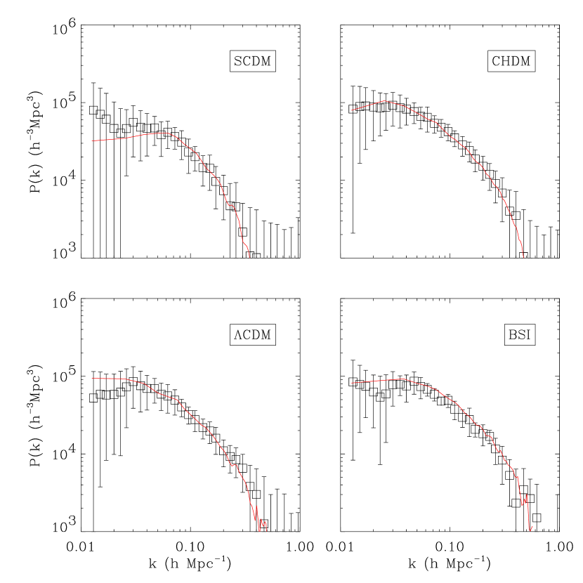
Figure 3: Comparison of the convolved power spectrum estimated from mock samples (square symbols) with the ‘real’ redshift space power spectrum from whole–box simulated catalogues (solid line).

We have calculated the mean value and the standard deviation of the power spectra within the set of mock samples available from the $N$–body simulations for each of the cosmological model. In order to assess the reliability of our method to estimate the power spectrum, we have compared the power spectrum $P(k)$ of simulated clusters in the periodic simulation box with the power spectrum estimate $\tilde{P}^{\prime}(k)$ of the mock catalogues. For the clusters in the periodic simulation cube a real–to–redshift space transformation along one dimension has been applied before.

In Fig. 3 the solid line denotes the mean $P(k)$ calculated from a number of simulations for the corresponding four cosmological models. The squares with error bars denote the mean of the convolution of the power spectrum $\tilde{P}^{\prime}(k)$ as found from the mock samples. First of all, this is a test for the correct implementation of the method. Moreover it provides an insight about the limitations of the method on the largest scales, where window convolution effects limit the reliability of the analysis. We conclude that the influences of the window on the reconstruction method is negligible for $k>0.03\,\mbox{$h\,{{\rm Mpc}}^{-1}$}$. In the following, we omit the tilde and prime on the convolution of the power spectrum with the window function.

We find that the variance between power spectra of different realizations is almost identical for different models. Therefore, we assume in the following the resulting cosmic scatter to be representative also for the observational results. Though this method closely resembles a Monte Carlo error estimation technique, we are restricted here to a smaller number of random realizations than usually employed. In the following we will take the $1\sigma$ scatter between the set of 64 CHDM mock samples as the error to be assigned to the Abell–ACO power spectrum since this model has the largest number of available realizations.

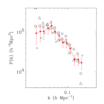
Figure 4: Redshift space cluster power spectrum for the Abell–ACO sample — filled circles, the Abell part — open circles, and the ACO part — diamonds (only southern–galactic part — triangles). The 1$\sigma$ error bars are derived from numerical simulations.

We show in Fig. 4 the results of the power spectrum reconstruction for the observational data. Open symbols refer to the different subsamples which have the same depth but cover different regions on the sky. Filled circles are for the combined Abell–ACO sample. For reasons of clarity, we plot error bars only for the latter. We find a general good agreement between the Abell and ACO parts (open circles and diamonds, respectively), and the combined sample, although ACO clusters show a slightly higher $P(k)$ on all scales. This result, which is consistent with the larger correlation length found for ACO clusters in previous analyses (e.g., Cappi & Maurogordato 1992; Plionis, Valdarnini & Jing 1992), can be attributed to a particular structure, the Shapley supercluster, which is located in the northern galactic part of the ACO sample. Excluding this region from the analysis (triangles) decreases the power spectrum amplitude (ACO–SG), although still within the cosmic variance error bars. Since each single subsample covers a smaller volume than the combined sample, finite volume effects start playing a role at smaller $k$ values (cf. Fig. 8, where we plot the window function shape for each subsample). Especially for ACO–SG, the amplitude at small wavenumbers is blown up. On scales $k>0.05\,\mbox{$h\,{{\rm Mpc}}^{-1}$}$ the spectrum may be approximated by a power law, $P(k)\propto k^{n}$ with negative index $n\simeq-1.9$. Going to larger scales, there is a clear evidence for a breaking of the power law. The transition is located at about $k\simeq 0.05\,\mbox{$h\,{{\rm Mpc}}^{-1}$}$ beyond which a power law with positive index could fit the data. Due to the large error bars, the scale of transition can not be pinned down very accurately.

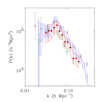
Figure 5: Comparison of various cluster power spectra obtained from 195 Abell clusters by Peacock & West (1992, crosses), 1304 Abell–ACO clusters by Einasto et al. (1997a, bars/dashed lines), 364 APM clusters by Tadros, Efstathiou & Dalton (1997, squares) and 417 Abell–ACO clusters (this work, dots and solid lines).

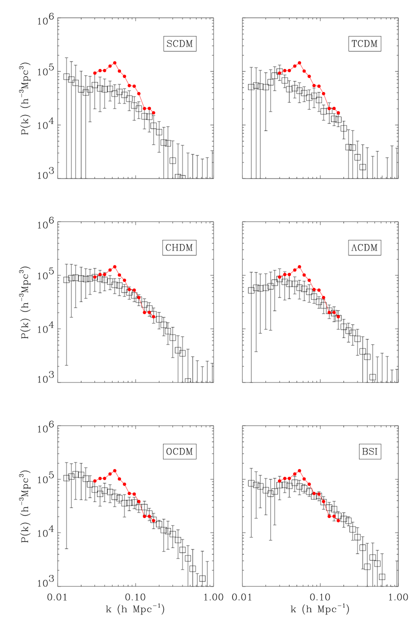
Figure 6: Power spectrum of the observed cluster sample (filled circles) compared with results obtained from mock cluster samples (squares) for six cosmological models. Error bars denote the $1\sigma$ variation over the mock samples.

Recently, the cluster power spectrum has been estimated for a sample of 1304 Abell/ACO clusters of galaxies by Einasto et al. (1997a). Differently from the analysis presented here, Einasto et al. (1997b) determined the large–scale behavior of the correlation function, and then used its Fourier transform as an estimate of the power spectrum. This method leads to a power spectrum with a pronounced peak at about $100\mbox{$h^{-1}{{\rm Mpc}}$}$ scale (see Fig. 5). The error corridor (indicated by dashed lines), which was also estimated from the correlation function, turns out to be narrower than our cosmic variance uncertainties. The parent cluster catalog analyzed by Einasto et al. (1997b) — the Abell–ACO catalog — is the same as ours. However, although the selection of $R\geq 0$ clusters within the angular boundaries dictated by galactic absorption is identical, the depth is different. Indeed, the sample used by Einasto et al. extends to a depth of 340 $h^{-1}{\rm{Mpc}}$ at the price of a higher fraction of non–spectroscopical cluster redshifts (33%), when compared to the 4% fraction of the sample we used here. Besides the difference in the observational data, we use different methods for estimating the power spectrum. In any case, the fact that the same $P(k)$ slope, $n\approx-1.9$, is found with both methods is a support to the robustness of this result. The maximum of $P(k)$ that we detect at $k=0.054\,\mbox{$h\,{{\rm Mpc}}^{-1}$}$ is somewhat less significant than, although consistent with, that found by Einasto et al. The significance of the peak is further decreased once the cosmic scatter is taken into account. The higher $P(k)$ amplitude found by Einasto et al. should be attributed to the different sample of 1304 clusters out to $340\,\mbox{$h^{-1}{{\rm Mpc}}$}$, and to uncertainties in the normalization of the 2–point correlation function that was used as the starting point of their analysis. In Fig. 5, we also show the previous results from Peacock & West (1992) for $R\geq 1$ Abell clusters. At wave numbers $k>0.08\,\mbox{$h\,{{\rm Mpc}}^{-1}$}$, the resulting $P(k)$ even tends to lie above the estimate by Einasto et al., as it should be expected on the ground of the higher richness of the clusters considered by Peacock & West (1992). Also their estimated errors are much smaller than ours, thus indicating the necessity to perform a large number of $N$–body simulations for estimating statistical uncertainty and cosmic variance. The power spectrum of rich clusters selected from the APM galaxy survey (Tadros, Efstathiou & Dalton 1997) turns out to be essentially consistent with our results. For wave numbers $k>0.04\,\mbox{$h\,{{\rm Mpc}}^{-1}$}$, the spectral amplitude is slightly smaller while the spectral slope is absolutely compatible. This consistency confirms the result based on the 2–point correlation function (cf. Fig. 2 and §3.1). It again indicates that Abell–ACO and APM cluster samples provide statistically equivalent descriptions of the local ($z\mathrel{\hbox{\hbox to0.0pt{\hbox{\lower 4.0pt\hbox{$\sim$}}\hss}\hbox{$<$}}}0.1$) cluster distribution.

In the following we will compare the power spectrum of the combined Abell–ACO sample with simulation results. In Fig. 6 the results from the mock samples (squares) are compared with the observational results (filled circles). Simulation results are the average over the available mock samples and error bars are the corresponding $1\sigma$ scatter between them. Only for SCDM, CHDM and $\Lambda$CDM error bars can be considered as a reliable representation of cosmic variance, since four, eight and three independent numerical realizations were carried out for these models, respectively. The predicted power spectrum of SCDM is too small on all scales. This confirms that the model definitely underproduces cluster clustering. Even by allowing for an overall vertical shift, the slope of the predicted spectrum is too shallow on intermediate scales $k=0.06-0.2\,\mbox{$h\,{{\rm Mpc}}^{-1}$}$. The TCDM model provides a nearly as worse fit as SCDM does. The CHDM model provides a good fit on small scales, but it underpredicts the $P(k)$ amplitude of the observational sample around the maximum, $0.04\mathrel{\hbox{\hbox to0.0pt{\hbox{\lower 4.0pt\hbox{$\sim$}}\hss}\hbox{$<$}}}k\mathrel{\hbox{\hbox to0.0pt{\hbox{\lower 4.0pt\hbox{$\sim$}}\hss}\hbox{$<$}}}0.07\,\mbox{$h\,{{\rm Mpc}}^{-1}$}$. Also the $\Lambda$CDM model is able to reproduce the power on large scales ($k\simeq 0.035\,\mbox{$h\,{{\rm Mpc}}^{-1}$}$) and small scales ($k\simeq 0.15\,\mbox{$h\,{{\rm Mpc}}^{-1}$}$) quite well, but it fails on intermediate scales having a too shallow slope. The OCDM model underpredicts cluster clustering by a similar amount as SCDM and TCDM. As for BSI, since error bars are likely to be slightly underestimated (just a single simulation realization is available), it provides the best fit to the data among the models we considered. However, even in this case, the overall shape of the observational $P(k)$ for $0.055\mathrel{\hbox{\hbox to0.0pt{\hbox{\lower 4.0pt\hbox{$\sim$}}\hss}\hbox{$<$}}}k\mathrel{\hbox{\hbox to0.0pt{\hbox{\lower 4.0pt\hbox{$\sim$}}\hss}\hbox{$<$}}}0.15\,\mbox{$h\,{{\rm Mpc}}^{-1}$}$ is steeper than for BSI clusters. We did not include the $\tau$CDM model into Fig. 6 because it is quite similar to the BSI model. This is not surprising since their linear spectra are almost identical.

In order to quantify the systematic discrepancy between the $P(k)$ shape for data and simulations, we performed a least–square fitting to the power law $P(k)\propto k^{n}$ in the above $k$ range. As a result, we find $n=-1.9\pm 0.2$ for the Abell–ACO sample, while $n=-1.3\pm 0.2$ (SCDM), $-1.2\pm 0.2$ (TCDM), $-1.3\pm 0.2$ (CHDM), $-1.2\pm 0.2$ ($\Lambda$CDM), $-1.0\pm 0.2$ (OCDM), $-1.1\pm 0.2$ (BSI), and $-1.1\pm 0.2$ ($\tau$CDM). At this level, we consider as premature to decide whether such a $\sim 2\sigma$ discrepancy between real data and mock samples is just due to a statistical fluctuation or is indicating an intrinsic problem for standard DM power spectra.

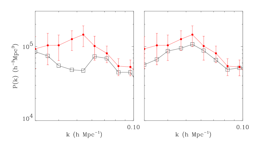
Figure 7: Power spectrum of the observed cluster sample (filled circles) and of two mock cluster samples (squares), extracted from the same simulation box. As in Fig. 4, error bars correspond to the estimated 1$\sigma$ cosmic scatter.

To illustrate this point we compare in Fig. 7 the power spectrum of two mock samples which have been extracted from the same simulation box. They represent the largest deviation between two mock samples of one simulation which we have found within the almost 20 simulations made. These mock samples clearly demonstrate the possible importance of cosmic variance, i. e. the fact that there is only one observational sample (for one special observer in the Universe). We conclude that a $P(k)$ as peaked as the observational one does not represent a very unusual finding. Therefore, the data may well be compatible with a power spectrum having a smooth turnover around $k\simeq 0.05\,h$ Mpc^-1, as expected for standard scenarios of structure formation, like those considered here.

On the other hand it is remarkable that Landy et al. (1996) also found a peak at about the same scale from the analysis of the Las Campanas Redshift Survey. Doroshkevich et al. (1997) found a typical scale of the same order in the Las Campanas Redshift Survey. Also the typical diameter of voids in the distribution of clusters is of the order of this scale (Gottlöber et al. 1997). Gaztañaga and Baugh (1998) found a steep slope for the real space power spectrum of APM galaxies in the same range as the unexpectedly steep slope of the cluster power spectrum. Eisenstein et al. (1998) concluded that an excess power on a $100\mbox{$h^{-1}{{\rm Mpc}}$}$ scale can be explained by baryonic acoustic oscillations only assuming rather extreme regions of the possible parameter space. Atrio–Barandela et al. (1997) and Lesgourgues et al. (1997) have discussed primordial spectra which include features that enable these models to account for a possible excess of power at $\sim 100\,h^{-1}$Mpc scales.

As for the bias parameter, we find that a larger $P(k)$ for the DM distribution does not correspond in general to a larger $P(k)$ for the resulting cluster distribution. Indeed, we find a remarkable amplification for the cluster power spectrum in the case of BSI, with a cluster biasing factor $b_{{\rm c}}^{2}\simeq 15$, while a much smaller enhancement occurs for SCDM, TCDM, CHDM, $\Lambda$CDM, and OCDM. This is consistent with the result that the cluster clustering does not depend on the amplitude of the underlying DM spectrum, but only on its shape, once the average number density of clusters is kept fixed (Croft & Efstathiou 1994; Borgani et al. 1997); the larger the large–to–small–scale power ratio, the larger the clustering amplification due to long wavelength modes. This is the reason why a model like BSI, which has a large relative amount of power on large scales and a low normalization, turns out to generate a highly biased cluster population.

6 Conclusion

In this paper we estimated the power spectrum, $P(k)$, for a combined redshift sample of Abell–ACO clusters. The result is compared with those obtained for mock cluster samples, which were extracted from large PM $N$–body simulations of seven different models, so as to reproduce the selection effects of the Abell–ACO data set. This analysis allows us not only to discriminate among different models for cosmic structure formation, but also to understand in detail the effect of cosmic variance on the power spectrum shape at the largest accessible scales.

The cluster power spectrum is reliably detected over the scale range $0.03\mathrel{\hbox{\hbox to0.0pt{\hbox{\lower 4.0pt\hbox{$\sim$}}\hss}\hbox{$<$}}}k\mathrel{\hbox{\hbox to0.0pt{\hbox{\lower 4.0pt\hbox{$\sim$}}\hss}\hbox{$<$}}}0.2\,\mbox{$h\,{{\rm Mpc}}^{-1}$}$, over which the analysis of cluster simulations demonstrates that the window function associated to the sample geometry has a negligible effect on $P(k)$. For $k\mathrel{\hbox{\hbox to0.0pt{\hbox{\lower 4.0pt\hbox{$\sim$}}\hss}\hbox{$>$}}}0.05\,\mbox{$h\,{{\rm Mpc}}^{-1}$}$ the cluster power spectrum is well approximated by a power law, $P(k)\propto k^{n}$ with $n\simeq-1.9$, while it changes sharply to a positive slope at smaller wavenumbers. We find a peak in the power spectrum at $k\simeq 0.05\,\mbox{$h\,{{\rm Mpc}}^{-1}$}$, which, however, is not as pronounced as the one detected by Einasto et al. (1997a).

The BSI model provides the best fit for the cluster power spectrum of Abell–ACO clusters among the models that we considered. In general, the models fail at about $2\sigma$ level at reproducing a $P(k)$ slope for $k\mathrel{\hbox{\hbox to0.0pt{\hbox{\lower 4.0pt\hbox{$\sim$}}\hss}\hbox{$>$}}}0.05\,\mbox{$h\,{{\rm Mpc}}^{-1}$}$ as steep as that of the Abell–ACO sample. Among the more than 100 mock samples that we extracted from the simulation boxes for the different models, we found that only one of them has a power spectrum with a feature almost identical to the observed one within the range $0.03\mathrel{\hbox{\hbox to0.0pt{\hbox{\lower 4.0pt\hbox{$\sim$}}\hss}\hbox{$<$}}}k\mathrel{\hbox{\hbox to0.0pt{\hbox{\lower 4.0pt\hbox{$\sim$}}\hss}\hbox{$<$}}}0.1\,\mbox{$h\,{{\rm Mpc}}^{-1}$}$. This finding shows the possible relevance of cosmic variance. It is just what one would expect for a feature, like the measured peak in the $P(k)$ shape, which represents a $2\sigma$ deviation from a smooth mean spectrum.

Observational samples which were both encompassing larger volumes and having selection effects under a strict control are required in order to decide whether details of the clustering pattern on a $100\mbox{$h^{-1}{{\rm Mpc}}$}$ scale force us to revise our understanding of structure formation or just leads to a refinement of the models which are already in play.

Appendix A The power spectrum estimation

In this Appendix we briefly describe the derivation of the power spectrum estimator, as given by Eq. (LABEL:final-estimator). The Abell–ACO cluster sample represents a three–dimensional catalogue which is almost complete (volume–limited) out to its boundaries. The selection effects arising from galactic absorption and redshift extinction are parameterized according to Eqs. (1) and (2). In order to estimate the power spectrum we employ the standard method, as described, e.g., by Fisher et al. (1993) and Lin et al. (1996).

The sample’s geometry is described by the window function $W(\vec{r})\equiv 1$ inside the sample volume and zero otherwise. Its Fourier transform has been computed by means of Monte Carlo integration. A total of $N=10^{5}$ random points with position vectors $\vec{r}_{i}\in V$ is generated to evaluate the Fourier representation of the window function $(1/N)\sum_{i}e^{i\vec{k}\cdot\vec{r}_{i}}$. The large number of points guarantees the noise level introduced into the power spectrum to be more than two decades below the noise level due to the finite number of galaxy clusters. Therefore, no correction for the shot noise contribution of the window function is applied.

Figure 8: Directional average of the window function (also called window power). The solid line corresponds to the Abell–ACO sample, the dashed and dotted lines describe Abell and ACO part separately (southern–galactic portion of the ACO sample (ACO–SG) — dash–dotted).

The double–cone geometry in real space with rotational symmetry about the $z$–axis (pointing towards the galactic pole) gives rise to a Fourier transform mostly localized along the $k_{z}$–axis and with cylindrical–symmetric side lobes in the $k_{x}$–$k_{y}$–plane. In Fig. 8 we have plotted the directional average $\langle|\hat{W}(\vec{k})|^{2}\rangle_{|\vec{k}|=k}$ for the combined Abell–ACO sample (solid line) and for the subsamples Abell (dashed), ACO (dotted) and ACO–SG (dash–dotted) separately. The maximum wavelength, whose power can be explored reliably, grows with the sample’s extension. Note that the depth of the three samples is all the same but the coverage of the celestial sphere is different. As a rule of thumb the minimum wavenumber $k_{{\rm min}}$ is given by $\langle|\hat{W}(\vec{k})|^{2}\rangle_{|\vec{k}|=k_{{\rm min}}}\equiv 0.1$ (Peacock & West 1992). This corresponds to wavenumbers $k_{{\rm min}}$ of 0.014, 0.017, 0.022 and $0.024\,\mbox{$h\,{{\rm Mpc}}^{-1}$}$ for the samples Abell–ACO, Abell, ACO and ACO–SG, respectively.

We define the cluster density contrast within the sampled volume as

$$\delta(\vec{r})\equiv\frac{1}{n}\sum_{i}\frac{\delta^{{\rm D}}(\vec{r}-\vec{r}_{i})}{\phi(\vec{r}_{i})}-1\,,$$ (5)

where $\vec{r}_{i}$ is the position vector of the $i$–th cluster, $\phi(\vec{r}_{i})$ is the selection function which is used to model galactic absorption and redshift extinction, $n$ is the mean cluster number density and $\delta^{{\rm D}}$ is Dirac’s delta function. The selection function is computed as the product

$$\phi(\vec{r})=D\varphi(b)\psi(z)\;,$$ (6)

with $D\simeq 0.7$ being the mean density correction applied to Abell clusters, while $D=1$ for ACO clusters.

The squared modulus of the Fourier transform $\delta(\vec{k})$ of the density contrast $\delta(\vec{r})$, $\Pi(\vec{k})$, is an estimate of the power spectrum. The connection between $\Pi(\vec{k})$ and the underlying power spectrum $P(k)$ can be found by calculating the ensemble mean of $\Pi(\vec{k})$ (see, e.g., Fisher et al. 1993 for the details),

$$\left\langle\Pi(\vec{k})\right\rangle\equiv\left\langle\left|\delta(\vec{k})\right|^{2}\right\rangle=\frac{\tilde{P}(\vec{k})}{V}+S\;,$$ (7)

where

$$\tilde{P}(\vec{k})\equiv\frac{V}{(2\pi)^{3}}\int{{\rm d}}^{3}k^{\prime}\,P(\vec{k^{\prime}})|\hat{W}(\vec{k^{\prime}}-\vec{k})|^{2}$$ (8)

denotes the convolution of the power spectrum with the window function and

$$S\equiv\frac{1}{nV^{2}}\int_{V}{{\rm d}}^{3}r\,\frac{1}{\phi(\vec{r})}\;.$$ (9)

the additive shot noise term. The ensemble average must be replaced with the best estimate $\Pi^{\prime}(k)$ that can be obtained from the data set. The mean number density is estimated from the data set as $n^{\prime}=V^{-1}\sum_{i}\phi(\vec{r}_{i})^{-1}$. Since $n^{\prime}$ may be in general different from the true mean number density of clusters, a bias in the power spectrum estimation is introduced (Peacock & Nicholson 1991). The spectrum is systematically underestimated by a factor of approximately $1-|\hat{W}(k)|^{2}$. A correction for this effect, which becomes relevant at scales approaching the largest scale covered by the sample, has been applied in Eq.(12). The shot noise (Eq. 9) is given by

$$S^{\prime}=\frac{1}{(n^{\prime}V)^{2}}\sum_{i}\frac{1}{\phi^{2}(\vec{r}_{i})}\;.$$ (10)

For each mode $k$ we compute the estimate $\Pi^{\prime}(k)$ by averaging $|\delta(\vec{k}_{j})|^{2}$ over M = 1000 random directions of the wavevector $|\vec{k}_{j}|=k$,

$$\Pi^{\prime}(k)=\frac{1}{M}\sum_{j}\left|\delta(\vec{k}_{j})\right|^{2},$$ (11)

Therefore, the estimator for the convolved power spectrum reads finally

$$\tilde{P}^{\prime}(k)=\frac{V}{1-|\hat{W}(k)|^{2}}\left[\Pi^{\prime}(k)-S^{\prime}\right]\;.$$ (12)

Inserting Eqs. (10) and (11) into Eq.(12) yields the convolved power spectrum Eq. (LABEL:final-estimator).

References

Abell G.O., 1958, ApJ, 3, 211

Abell G.O., Corwin H.G., Olowin R.P., 1989, ApJS, 70, 1

Amendola L., Gottlöber S., Mücket J.P., Müller V., 1995, ApJ, 457, 444

Andernach H., Tago E., Stengler–Larrea E., 1995, Astrophys. Lett. & Comm., 31, 27

Atrio–Barandela F., Einasto J., Gottlöber S., Müller V., Starobinsky A.A., 1997, JETP Letters, 66, 367

Bahcall N.A., Soneira R.M., 1983, ApJ, 270, 20

Batuski D.J., Bahcall N.A., Olowin R.P., Burns, J.O., 1989, ApJ, 341, 599

Bardeen J.M., Bond J.R., Kaiser N., Szalay A.S., 1986, ApJ, 304, 15

Bennett C.L. et al., 1994, ApJ, 436, 423

Borgani S., Plionis M., Coles P., Moscardini L., 1995, MNRAS, 277, 1191

Borgani S., Moscardini L., Plionis M., Górski K.M., Holtzman J., Klypin A., Primack J.P., Smith C.C., 1997, NewA, 1, 321

Cappi A., Maurogordato S., 1992, A&A, 259, 423

Collins C.A., Guzzo L., Nichol R.C., Lumsden S.L., 1995, MNRAS, 274, 1071

Croft R.A.C., Efstathiou G., 1994, MNRAS, 267, 390

Croft R.A.C., Dalton G.B., Efstathiou G., Sutherland W.J., Maddox S.J., 1997, MNRAS, 291, 305

Dalton G.B., Croft R.A.C., Efstathiou G., Sutherland W.J., Maddox S.J., Davis M., 1994, MNRAS, 271, L47

Doroshkevich A. G., Tucker D.L., Oemler A. JR., Kirshner R.P., Lin H., Shectman S.A., Landy S.D., Fong R., 1996, MNRAS, 283, 1281

Ebeling H., Edge A.C., Fabian A.C., Allen S.W., Crawford C.S., 1997, ApJ, 479, L101

Efstathiou G.P., Bond J.R., White S.D.M., 1992a, MNRAS, 258, 1P

Efstathiou G., Dalton G.B., Sutherland W.J., Maddox S.J., MNRAS, 1992b, 257, 125

Einasto J., Gramann M., Saar E., Tago E., 1993, MNRAS, 260, 705

Einasto J., Einasto M., Gottlöber S., Müller V., Saar V., Starobinsky A.A., Tago E., Tucker D., Andernach H., Frisch P., 1997a, Nature, 385, 139

Einasto J., Einasto M., Frisch P., Gottlöber S., Müller V., Saar V., Starobinsky A.A., Tago E., Tucker D., Andernach H., 1997b, MNRAS, 289, 801

Eisenstein D.J., Hu W., Silk J., and Szalay A.S., 1998, ApJ, 494, 1

Feldman H.A., Kaiser N., Peacock J.A., 1994, ApJ, 426, 23

Fisher K.B., Davis M., Strauss M.A., Yahil A., Huchra J.P., 1993, ApJ, 402, 42

Gaztañaga E., Baugh C.M., 1998, MNRAS, 294, 229

Gaztañaga E., Croft R.A.C., Dalton G.B., 1995, MNRAS, 276, 336

Ghigna S., Bonometto S.A., Retzlaff J., Gottlöber S., Murante G., 1996, ApJ, 469, 40

Górski K.M., Banday A.J., Bennett C.L., Hinshaw G., Kogut A., Smoot G.F., Wright E.L., 1996, ApJ, 464, L11 (G96)

Górski K.M., Ratra B. Stompor R., Sugiyama N., Banday A.J., 1998, ApJS, 114, 1 (G98)

Gottlöber S., 1996, Proceedings of the International School of Physics ”Enrico Fermi”, eds. S. Bonometto, J.R. Primak, A. Provenzale, IOS Press, Amsterdam, p. 467

Gottlöber S., Müller V., Starobinsky A.A., 1991, Phys. Rev. D43, 2510

Gottlöber S., Mücket J.P., Starobinsky A.A., 1994, ApJ, 434, 417

Gottlöber S., Retzlaff J., Turchaninov V., 1997, Astrophysics Reports 2, 55.

Jenkins A. et al. (The Virgo Consortium), 1998, ApJ, 499, 20

Jing Y.P., Plionis M., Valdarnini R., 1992, ApJ, 389, 499

Jing Y.P., Valdarnini R., 1993, ApJ, 406, 6

Kates R., Müller V., Gottlöber S., Mücket J.P., Retzlaff J., 1995, MNRAS, 277, 1254

Kerscher M., Schmalzing J., Retzlaff J., Borgani S., Buchert T., Gottlöber S., Müller V., Plionis M., Wagner H., 1997, MNRAS, 284, 73

Klypin A., Kopylov A.I., 1983, Soviet Astron. Lett., 9, 41

Klypin A., Rhee G., 1994, ApJ, 428, 399

Klypin A., Gottlöber S., Kravtsov A., Khokhlov A., 1997, astro–ph/9708191

Landy S.D., Shectman S.A., Lin H.L., Kirshner R.P., Oemler A., Tucker D.L., Schechter P.L., 1996, ApJ, 456, L1

Lesgourgues J., Polarski D., Starobinsky A. A., 1998, MNRAS, 297, 769

Lin H.L., Kirshner R.P., Shectman S.A., Landy S.D., Oemler A., Tucker D.L., Schechter P.L., 1996, ApJ, 471, 617

Lucchin F., Matarrese S., 1985, Phys. Rev., D32, 1316

Nichol R.C., Briel U.G., Henry J.P., 1994, MNRAS, 265, 867

Nichol R.C., Connolly A.J., 1996, MNRAS, 279, 521

Olivier S.S., Primack J.R., Blumenthal G.R., Dekel A., 1993, ApJ, 408, 17

Park C., Vogeley M.S., Geller M.J., Huchra J.P., 1994, ApJ, 431, 569

Peacock J.A., Nicholson D., 1991, MNRAS, 253, 307

Peacock J.A., West M.J., 1992, MNRAS, 259, 494

Plionis M., Valdarnini R., 1991, MNRAS, 249, 46

Plionis M., Valdarnini R., 1995, MNRAS, 272, 869

Plionis M., Valdarnini R., Jing Y.P., 1992, ApJ, 398, 12

Postman M, Huchra J.P., Geller M., 1992, ApJ, 384, 407

Primack J., Holtzman J., Klypin A., Caldwell D., 1995, Phys. Rev. Lett. 74, 2160

Ratra B., Peebles, P.J.E., 1994, ApJ, 432, L5

Romer A.K., Collins C.A., Böhringer H., Cruddace R.C., Ebeling H., MacGillawray H.T., Voges W., 1994, Nature, 372, 75

Scaramella R., Zamorani G., Vettolani G., Chincarini G., 1991, AJ, 101, 342

Schuecker P., Ott H.–A., Seitter W.C., 1996, ApJ, 472, 485

Strauss M.A., Willick J.A., 1995, Phys. Rep., 261, 271

Sutherland W.J., 1988, MNRAS, 234, 159

Tadros H., Efstathiou G., 1996, MNRAS, 282, 1381

Tadros H., Efstathiou G., Dalton G., 1998, MNRAS, 296, 995

Viana P.T.P, Liddle A.R., 1996, MNRAS, 281, 323 (V96)

White M., Gelmini G., Silk J., (1995), Phys. Rev. D51, 2669

Wilson M.L., 1983, ApJ, 273, 2.