BEYOND ZEL’DOVICH-TYPE APPROXIMATIONS IN GRAVITATIONAL INSTABILITY THEORY
— Padé Prescription in Spheroidal Collapse —

Abstract

Among several analytic approximations for the growth of density fluctuations in the expanding Universe, Zel’dovich approximation in Lagrangian coordinate scheme is known to be unusually accurate even in mildly non-linear regime. This approximation is very similar to the Padé approximation in appearance. We first establish, however, that these two are actually different and independent approximations with each other by using a model of spheroidal mass collapse. Then we propose Padé-prescribed Zel’dovich-type approximations and demonstrate, within this model, that they are much accurate than any other known nonlinear approximations.

When we analyze the growth of density fluctuations in the expanding Universe by analytical methods, the Zel’dovich-type approximations (ZTA hereafter) are known to be unusually accurate even in mildly non-linear regime for unknown reason [1, 2, 3, 4, 5, 6, 7, 8]. These Zel’dovich-type approximations are grounded on the Lagrangian coordinate scheme and are one-dimensional-exact; they become exact in the plain parallel mass distributions. The validity of ZTA has been argued recently based on these physical properties [9]. On the other hand, the appearance of these ZTA are very similar to the rational expansion method called Padé approximations. Though they have been widely used in the literature, the validity of these approximations has not yet been established as well.

We would like first to compare these Zel’dovich-type and Padé approximation methods. It is almost impossible and is not pragmatic to argue in general analytic form. Therefore in this letter, we restrict our consideration to a model of spheroidal collapse which we can solve semi-analytically. If the above two types of approximations are actually the same, then they would give the same result for this restricted model. We demonstrate, in the first part of this letter, that this is not the case and conclude that they are independent approximation schemes. Then this fact suggests a possibility to go beyond ZTA by Padé prescription on ZTA. We demonstrate, in the second part of this letter, that this Padé prescription dramatically improves ZTA.

In the gravitational instability theory, the non-relativistic matter with zero pressure in an Einstein-de Sitter (EdS) universe is described by the following set of equations (see Ref. [10]),

$$\dot{\delta}+\nabla\cdot[(1+\delta){\mbox{\boldmath$v$}}]=0,$$ (1)

$$\dot{{\mbox{\boldmath$v$}}}+2H{\mbox{\boldmath$v$}}+({\mbox{\boldmath$v$}}\cdot\nabla){\mbox{\boldmath$v$}}+\nabla\Phi=\bf 0,$$ (2)

$$\nabla^{2}\Phi=\frac{3}{2}H^{2}\delta,$$ (3)

where $x$, ${\mbox{\boldmath$v$}}({\mbox{\boldmath$x$}},t)$, $\Phi({\mbox{\boldmath$x$}},t)$ are respectively position, peculiar velocity, peculiar potential in comoving coordinate. The scale factor $a$ varies as $a\propto t^{2/3}$ and the Hubble parameter is $H=\dot{a}/a=2/(3t)$. Although we consider only EdS universe for simplicity in this letter, it is straightforward to generalize the analyses in general Friedman-Lemître universes.

In the Eulerian coordinate scheme, the linear solution of them has a simple form $\delta_{\rm L}({\mbox{\boldmath$x$}},t)=\delta_{\rm in}({\mbox{\boldmath$x$}})a(t)/a_{\rm in}$, neglecting the decaying mode. Considering this to be a small parameter, we can naturally expand the full solution in powers of $\delta_{\rm L}$: $\delta=\delta_{\rm L}+\delta^{(2)}+\delta^{(3)}+\cdots$, $\Phi=\Phi_{\rm L}+\Phi^{(2)}+\Phi^{(3)}+\cdots$, ${\mbox{\boldmath$v$}}={\mbox{\boldmath$v$}}_{\rm L}+{\mbox{\boldmath$v$}}^{(2)}+{\mbox{\boldmath$v$}}^{(3)}+\cdots$, where $\delta^{(n)}$, $\Phi^{(n)}$, ${\mbox{\boldmath$v$}}^{(n)}$ are assumed to be of order $(\delta_{\rm L})^{n}$. (e.g., see [10, 11, 12]).

In the Zel’dovich-type approximations [1, 3, 8, 13, 14, 15], we work in the Lagrangian coordinate scheme in which the location of a mass element $x$ of the fluid is expressed by the initial location $q$ and the time dependent displacement vector $\Psi$ as ${\mbox{\boldmath$x$}}({\mbox{\boldmath$q$}},t)={\mbox{\boldmath$q$}}+{\mbox{\boldmath$\Psi$}}({\mbox{\boldmath$q$}},t)$. Then the density contrast $\delta[{\mbox{\boldmath$x$}}({\mbox{\boldmath$q$}},t),t]=\det[\partial x_{i}/\partial q_{j}]^{-1}-1$ is determined by solving the equation of motion

$$\left[\frac{d^{2}{\mit\Psi}_{i,j}}{dt^{2}}+2H\frac{d{\mit\Psi}_{i,j}}{dt}\right]\left(J^{-1}\right)_{ji}+\frac{3}{2}H^{2}\left(J^{-1}-1\right)=0,$$ (4)

$$\epsilon_{ijk}\frac{d{\mit\Psi}_{j,l}}{dt}\left(J^{-1}\right)_{lk}=0,$$ (5)

where $d/dt$ is the Lagrangian time derivative, $J_{ij}=\partial x_{i}/\partial q_{j}=\delta_{ij}+{\mit\Psi}_{i,j}$, $J=\det J_{ij}$. This Eq. (4) is obtained from Eqs. (2) and (3), and Eq. (5) corresponds to the usual Eulerian vorticity-free condition. These nonlinear equations for $\Psi$ can be solved by the method of iteration considering $\partial{\mit\Psi}_{i}/\partial q_{j}$ as small expansion parameter: ${\mit\Psi}_{i,j}={\mit\Psi}_{i,j}^{(1)}+{\mit\Psi}_{i,j}^{(2)}+{\mit\Psi}_{i,j}^{(3)}+\cdots$. In EdS universe, the time dependence of each terms is separated from its spatial dependence: ${\mbox{\boldmath$\Psi$}}^{(n)}=(2/(3a^{2}H^{2}))^{n}{\mbox{\boldmath$\psi$}}^{(n)}({\mbox{\boldmath$q$}})$. The first-order solution $\psi^{(1)}_{i}=-\partial_{i}\phi_{\rm L}({\mbox{\boldmath$q$}})$ is the original Zel’dovich approximation (ZA).

Now we introduce a model of collapsing homogeneous ellipsoid. We parameterize the density perturbation $\delta({\mbox{\boldmath$x$}},t)$ as

$$\delta({\mbox{\boldmath$x$}},t)=\delta_{\rm e}(t)\,\,\,\Theta\left(1-\frac{x_{1}^{\,2}}{\alpha_{1}^{\,2}(t)}-\frac{x_{2}^{\,2}}{\alpha_{2}^{\,2}(t)}-\frac{x_{3}^{\,2}}{\alpha_{3}^{\,2}(t)}\right),$$ (6)

where $\alpha_{i}$ are the half-length of the principal axes of the ellipsoid and $\Theta$ is the step function. The solution of the Poisson Eq. (3) inside this homogeneous ellipsoid is known (see, Ref. [16]) and it becomes $\Phi=\frac{3}{8}H^{2}\delta_{\rm e}\sum_{i=1}^{3}A_{i}(t)x_{i}^{\,2}$, and the equations of motion for three $\alpha_{i}$ are given by [9, 17]

$$\ddot{\alpha}_{i}+2H\dot{\alpha}_{i}=-\frac{3}{4}H^{2}\delta_{\rm e}A_{i}\alpha_{i},$$ (7)

where

$$A_{i}=\alpha_{1}\alpha_{2}\alpha_{3}\int_{0}^{\infty}(\alpha_{i}^{\,2}+\lambda)^{-1}\prod_{j=1}^{3}(\alpha_{j}^{\,2}+\lambda)^{-1/2}d\lambda.$$ (8)

The density contrast of the ellipsoid is obtained by observing that $1+\delta$ is inversely proportional to $\alpha_{1}\alpha_{2}\alpha_{3}$. These equations are solved by numerical integration. The solutions are ’semi-analytic’ in this sense. In the following, we only consider spheroidal case, $\alpha_{1}=\alpha_{2}$ for simplicity.

For the system of spheroidal perturbations, we apply ZTA, resulting in [9]

$$\psi^{(1)}_{(1,2)}=\mp\displaystyle\frac{a^{3}H^{2}q_{(1,2)}}{2}(1+h_{\rm in}),$$ (9)

$$\psi^{(1)}_{3}=\mp\displaystyle\frac{a^{3}H^{2}q_{3}}{2}(1-2h_{\rm in}),$$ (10)

$$\psi^{(2)}_{(1,2)}=-\displaystyle\frac{3a^{6}H^{4}q_{(1,2)}}{28}(1+h_{\rm in}-h_{\rm in}^{2}-h_{\rm in}^{3}),$$ (11)

$$\psi^{(2)}_{3}=-\displaystyle\frac{3a^{6}H^{4}q_{3}}{28}(1-2h_{\rm in}-h_{\rm in}^{2}+2h_{\rm in}^{3}),$$ (12)

$$\psi^{(3)}_{(1,2)}=\mp\displaystyle\frac{a^{9}H^{6}q_{(1,2)}}{504}(23+23h_{\rm in}-39h_{\rm in}^{2}$$ (13)

$$\qquad\qquad\qquad\qquad\qquad-25h_{\rm in}^{3}+44h_{\rm in}^{4}+30h_{\rm in}^{5}),$$ (14)

$$\psi^{(3)}_{3}=\mp\displaystyle\frac{a^{9}H^{6}q_{3}}{504}(23-46h_{\rm in}-39h_{\rm in}^{2}$$ (15)

$$\qquad\qquad\qquad\qquad+92h_{\rm in}^{3}+2h_{\rm in}^{4}-60h_{\rm in}^{5}),$$ (16)

where we have changed the parametrization, $A_{1}=A_{2}=\frac{2}{3}(1+h)$, $A_{3}=\frac{2}{3}(1-2h)$ [18], and $h_{\rm in}=h(t_{\rm in})$, with $t_{\rm in}$ being the initial time for numerical integration. The density contrast in these ZTA is given by

$$\delta=\frac{q_{1}q_{2}q_{3}}{(q_{1}+{\mit\Psi}_{1})(q_{2}+{\mit\Psi}_{2})(q_{3}+{\mit\Psi}_{3})}-1,$$ (17)

where ${\mit\Psi}_{i}={\mit\Psi}^{(1)}_{i}$ corresponds to the original ZA, ${\mit\Psi}_{i}={\mit\Psi}^{(1)}_{i}+{\mit\Psi}^{(2)}_{i}$ corresponds to post-Zel’dovich approximation (PZA), ${\mit\Psi}_{i}={\mit\Psi}^{(1)}_{i}+{\mit\Psi}^{(2)}_{i}+{\mit\Psi}^{(3)}_{i}$ corresponds to post-post-Zel’dovich approximation (PPZA).

In contrast to the above Lagrangian perturbation methods, the surface of the spheroid cannot be explicitly expressed in Eulerian perturbation methods. We simply transform the expression already obtained in Lagrangian perturbation scheme to that in Eulerian perturbation scheme. This is based on the fact that the small expansion parameters ${\mit\Psi}_{i,j}$ in Lagrangian scheme and $\delta$ in Eulerian scheme are the same order and thus ${\mit\Psi}^{(n)}_{i,j}\ \sim\delta^{(n)}$. In our case, ${\mit\Psi}^{(n)}\propto a^{n}$, so Eulerian perturbative series can be simply obtained by expanding equation (17) in terms of expansion factor $a$:

$$\delta=\pm a+\left(\frac{17}{21}+\frac{4}{21}h_{\rm in}^{2}\right)a^{2}$$ (18)

$$\qquad\pm\left(\frac{341}{567}+\frac{74}{189}h_{\rm in}^{2}-\frac{4}{81}h_{\rm in}^{3}-\frac{8}{189}h_{\rm in}^{4}\right)a^{3}.$$ (19)

Now we introduce Padé approximation associated with the Perturbative expansions in Eulerian coordinate scheme. Padé approximation of type-$(M,N)$ for a given unknown function $f(x)$ is expressed as the ratio of two polynomials.

$$f_{\mbox{Pad\'{e}}(M,N)}\equiv\left(\displaystyle\sum_{k=0}^{M}a_{k}x^{k}\right)\left(1+\displaystyle\sum_{k=1}^{N}b_{k}x^{k}\right)^{-1}.$$ (20)

The constant parameters $a_{k}$ and $b_{k}$ are determined so that they maximally yield the known Taylor expansion of the function $f(x)$ [19] up to $(M+N)$-th order. The density contrast in the spheroidal model up to the third-order perturbation is given by Eq. (19). The corresponding Padé approximation of type-(1,2) is given by

$$\delta=\pm a\left[1\mp\displaystyle\frac{17+4h_{\rm in}^{2}}{21}a\right.$$ (21)

$$\quad\left.+\left(\displaystyle\frac{214}{3969}-\frac{110}{1323}h_{\rm in}^{2}+\frac{4}{81}h_{\rm in}^{3}+\frac{104}{1323}h_{\rm in}^{4}\right)a^{2}\right]^{-1}.$$ (22)

We observe that the ZTA density contrast of Eq. (17) and Padé density contrast of Eq. (22) are definitely different with each other. Actually the plots of these approximations in Fig. 1 for spherical perturbations clearly demonstrate the difference. Some of lines in Fig. 1 have been previously appeared [3, 5].

FIG. 1.: Density contrasts in Eulerian approximations and ZTA and their corresponding Padé approximations in the model of spherical density perturbations. Vertical axis is the density contrasts $\delta_{\rm approx}$ of each approximations and the horizontal axis is the true solution $\delta_{\rm true}$. Fig. 1(a) is for a case of positive perturbation and Fig. 1(b) is for a case of negative perturbation.

Since the Zel’dovich-type approximations and Padé approximations are different scheme with each other, we may be able to invent better approximations by combining these two scheme. In doing so, we notice that the each factor ${\mit\Psi}_{i}$ in Eqs. (9)-(16) has an appropriate series expansion form. Therefore we apply Padé approximation for these factors ${\mit\Psi}_{i}$ separately. For example, Padé approximation for the factor ${\mit\Psi}_{1}$ becomes

$${\mit\Psi}_{1\,\mbox{Pad\'{e}}(1,2)}=\mp\frac{a(1+h_{\rm in})q_{1}}{3}\left[1\mp\displaystyle\frac{a(1-h_{\rm in}^{2})}{7}\right.$$ (23)

$$\qquad\qquad\left.-\displaystyle\frac{a^{2}(80-111h_{\rm in}^{2}+98h_{\rm in}^{3}+129h_{\rm in}^{4})}{3969}\right]^{-1},$$ (24)

$${\mit\Psi}_{1\,\mbox{Pad\'{e}}(2,1)}=\mp\frac{a(1+h_{\rm in})q_{1}}{21}\times$$ (25)

$$\quad\left[567(1-h_{\rm in})\right.\left.\mp a(80-80h_{\rm in}-31h_{\rm in}^{2}+129h_{\rm in}^{3})\right]\times$$ (26)

$$\quad\left[81(1-h_{\rm in})\right.\left.\mp a(23-23h_{\rm in}-16h_{\rm in}^{2}+30h_{\rm in}^{3})\right]^{-1},$$ (27)

where we employed Padé approximation of type-(1,2) and type-(2,1) in Eqs. (24) and (27), respectively.

We show the result of these Padé-prescribed PZA and PPZA (PadéPZA, PadéPPZA hereafter) in Figs. 2 and 3 as well as other non-linear approximations. Since the relative accuracy of various approximations is almost the same for all values of $\delta_{\rm true}$, we have decided to fix $\delta_{\rm true}$ and show the accuracy of approximations for various values of $\alpha_{\rm in3}/\alpha_{\rm in1}$ at once. In Fig. 2, the density contrasts of various approximations in spheroidal collapse of positive perturbations are shown. The horizontal axis represents the initial axis-ratio $\alpha_{\rm in3}/\alpha_{\rm in1}$; oblate configuration for $\alpha_{\rm in3}/\alpha_{\rm in1}<1$, and prolate configuration for $\alpha_{\rm in3}/\alpha_{\rm in1}>1$. The case $\alpha_{\rm in3}/\alpha_{\rm in1}=1$ corresponds to the spherical configuration shown in Fig. 1. The vertical axis in Fig. 2 represents the ratio of the density contrasts $\delta_{\rm approx}/\delta_{\rm true}$ evaluated at $\delta_{\rm true}=4$ well within the non-linear regime. Both the axis ratio and density ratio are in logarithmic scale in this figure. In Fig. 3, we plotted the same graph as Fig. 2 but for negative perturbations. The density contrast $\delta_{\rm approx}/\delta_{\rm true}$ in the negative perturbation model is evaluated at $\delta_{\rm true}=-0.6$.

We observe from these figures the following facts:

• PadéPPZA constantly yields the best precision among various approximation scheme for all initial axes-ratio $\alpha_{\rm in~{}3}/\alpha_{\rm in~{}1}$ in both positive and negative spheroidal perturbations.

• The Padé-prescription results in much dramatic improvement in precision in the negative perturbations than positive perturbations

• All the graph seems to converge to the exact solution in the oblate limit.

The above facts (i) and (ii) demonstrate the excellence of the Padé prescription for ZTA. Especially the negative perturbation case is remarkable. For example, the Padé prescription improves the PPZA about factor six for $\delta_{\rm true}=-0.6$. The last fact (iii) simply reflects that Padé approximations as well as Zel’dovich-type approximations have the one-dimensional-exact property. Actually the limit of one-dimensional collapse is achieved by setting $h_{\rm in}\rightarrow-1$. In this limit, the Eq. (22) reduces to the exact solution, $\delta=\pm a/(1\mp a)$. Therefore the Padé approximation in the present model also has the one-dimensional-exact property as ZTA.

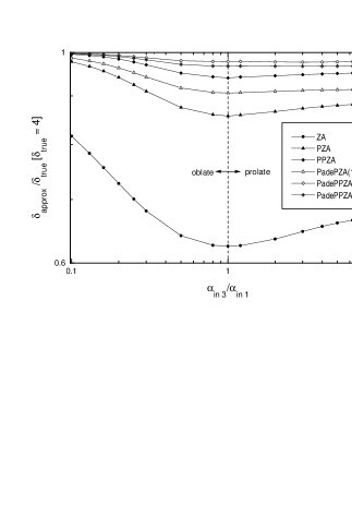
FIG. 2.: Density contrasts of various approximations in spheroidal collapse of positive perturbations. The horizontal axis represents the initial axis-ratio $\alpha_{\rm in3}/\alpha_{\rm in1}$ and the vertical axis represents the ratio of density contrast $\delta_{\rm approx}/\delta_{\rm true}$ evaluated at $\delta_{\rm true}=4$. Both the axis ratio and density ratio are in logarithmic scale in this figure.

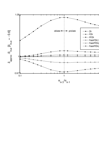
FIG. 3.: The same graph as Fig. 2 but for negative perturbations. The vertical axis represents the ratio of density contrast $\delta_{\rm approx}/\delta_{\rm true}$ evaluated at $\delta_{\rm true}=-0.6$.

Now we conclude our work. First we focused on the issue that ZTA and Padé approximations are actually the same scheme or not. By using spheroidal perturbation models, we found that these two types of approximations are different independent scheme with each other despite the similar appearance. Then, based on this fact, we proposed the Padé prescription for the ZTA. We found this Padé prescription appreciably increases the accuracy of ZTA.

This Padé-prescribed ZTA may shed light on the practical calculations on the evolution of density perturbations in the Universe.

The Padé approximation for PPZA we used is not the pure original form of the scheme. Actually we Padé-prescribed the part of denominator of the density perturbations $\delta$ in Eq. (17). This reminds us the continued fraction approximation. We hope these Padé and continued fraction approximation scheme may reveal the true validity of the ZTA in the future.

REFERENCES

[1] Ya. B. Zel’dovich, Astron. Astrophys. 5,
84 (1970).
[2] Ya. B. Zel’dovich, Astrophysics 6, 164
(1973).
[3] D. Munshi, V. Sahni and A. A. Starobinsky,
Astrophys. J. 436, 517 (1994).
[4] V. Sahni and P. Coles, Phys. Rep. 262, 1 (1995).
[5] V. Sahni and S. Shandarin,
Mon. Not. R. Astron. Soc. 282, 641 (1996).
[6] T. Buchert, A. L. Melott and A. G. Weiss,
Astron. Astrophys. 288, 349 (1994).
[7] A. L. Melott, T. Buchert and A. G. Weiss,
Astron. Astrophys. 294, 345 (1995).
[8] F. R. Bouchet, S. Colombi, E. Hivon and
R. Juszkiewicz, Astron. Astrophys. 296, 575 (1995).
[9] A. Yoshisato, T. Matsubara and M. Morikawa, Report
No. astro-ph/9707296.
[10] P. J. E. Peebles, The Large-Scale Structure of
Universe (Princeton Univ.Press, Princeton, 1980).
[11] J. N. Fry, Astrophys. J. 279, 499 (1984).
[12] M. H. Goroff, B. Grinstein, S.-J. Rey and M. B. Wise,
Astrophys. J. 311, 6 (1986).
[13] T. Buchert and J. Ehlers,
Mon. Not. R. Astron. Soc. 264, 375 (1993).
[14] T. Buchert Mon. Not. R. Astron. Soc. 267,
811 (1994).
[15] P. Catelan, Mon. Not. R. Astron. Soc. 276, 115
(1995).
[16] O. Kellogg, Foundation of Potential Theory
(Dover, New York, 1995).
[17] S. D. M. White and J. Silk, Astrophys. J. 231, 1
(1979).
[18] The coefficients automatically satisfy the
constraint , which follows from Poisson
Eq. (3).
[19] C. M. Bender and S. A. Orszag, Advanced
Mathematical Methods for Scientists and Engineers (McGraw-hill Book
Company, New York, 1978).