The Norris Survey of the Corona Borealis Supercluster:
III. Structure and Mass of the Supercluster

Abstract

We present a study of the structure and dynamics of the Corona Borealis Supercluster ($z\approx 0.07$) based on the redshifts of 528 galaxies in the supercluster. The galaxy distribution within Corona Borealis is clumpy and appears overall to be far from relaxed. Approximately one-third of the supercluster galaxies lie outside of the Abell clusters in the supercluster. A background supercluster at $z\approx 0.11$ makes a substantial contribution to the projected surface density of galaxies in the Corona Borealis field. In order to estimate the mass of the supercluster, we have assumed that the mass of the supercluster is proportional to $v^{2}r$, where $v$ and $r$ are suitable scale velocity and radius, respectively, and we have used $N$-body simulations of both critical- and low-density universes to determine the applicability of standard mass estimators based on this assumption. Although superclusters are obviously not in equilibrium, our simulations demonstrate that the virial mass estimator yields mass estimates with an insignificant bias and a dispersion of only $\sim 25$% for objects with overdensities $\gtrsim 5$. Non-uniform spatial sampling can, however, cause systematic underestimates of as much as 30%. The projected mass estimator (Bahcall & Tremaine 1981) is less accurate but still provides useful estimates in most cases. All of our simulated superclusters turn out to be bound, and based on the overdensity of the Corona Borealis supercluster, we believe it is also very likely to be bound and may well have started to collapse. The mass of Corona Borealis is at least $3\times 10^{16}h^{-1}M_{\sun}$ ($h$ is the Hubble constant in units of 100 km s^-1 Mpc^-1) , which yields a $B_{AB}$-band mass-to-light ratio of $564h{M\overwithdelims( )L}_{\sun}$ on scales of $\sim 20h^{-1}$ Mpc. The background supercluster has a similar mass-to-light ratio of $726h{M\overwithdelims( )L}_{\odot}$. By comparing the supercluster mass-to-light ratios with the critical mass-to-light ratio required to close the universe, we determine that $\Omega_{0}\gtrsim 0.4$ on supercluster scales.

1 Introduction

Abell (1958), from his survey of galaxy clusters in the Palomar Observatory Sky Survey, was the first to note the existence of clusters of clusters of galaxies, which he called “second order clusters” and which have since been dubbed “superclusters.” They are among the largest identified objects in the universe but are only $\sim 5$ to $\sim 40$ times denser than the field (Small, Sargent, & Hamilton 1997a, Paper II in the current series). In contrast, the overdensity of an object that has just become virialized is $\sim 200$, and the overdensity in the center of an Abell cluster is $\sim 1000$. Since the dynamical times of superclusters are comparable to the Hubble time, superclusters are not relaxed and should therefore bear the imprints of the physical processes that were dominant during their formation. One hopes that studies of superclusters will ultimately yield information about the nature of density fluctuations. In addition, since superclusters are mildly or modestly non-linear, the structure of superclusters may offer clues about the growth of structure. In this paper, we describe our efforts to use dynamical studies of superclusters to provide insights into the distribution of matter on large scales.

Knowledge of the mass distribution on large scales is, of course, essential for determining $\Omega_{0}$, the ratio of the present-day matter density of the universe to the critical density required for a closed universe. On the scales of rich clusters of galaxies ($\sim 1h^{-1}$ Mpc, where $h$ is the Hubble constant in units of 100 km s^-1 Mpc^-1), $\Omega_{0}$ may be estimated by comparing the mass-to-light ratio ($M/L$ ratio) of virialized clusters with the $M/L$ ratio required to close the universe (e.g., Gunn 1978; Kent & Gunn 1982; Kent & Sargent 1983; Sharples, Ellis, & Gray 1988). The comprehensive work by Carlberg et al. (1996, 1997) based on 14 rich clusters yields $M/L=213\pm 59h{M\overwithdelims( )L}_{\odot}$ in the $r$ band, which in turn gives $\Omega_{0}=0.19\pm 0.06\pm 0.04$ (formal 1 $\sigma$ random errors and estimated systematic errors), well short of the matter density required to close the universe. However, measurements of $\Omega_{0}$ on larger scales ($\sim 10-100h^{-1}$ Mpc) from velocity flows and redshift-space distortions tend to favor larger values, although with large error bars. (See Dekel, Burstein, & White 1996 for a review.) The dynamics of superclusters offer an important independent means of estimating $\Omega_{0}$ on $\sim 20h^{-1}$ Mpc scales. Here, we present a measurement of the $M/L$ ratio of the Corona Borealis supercluster, and thus a measurement of $\Omega_{0}$, based on data from a large redshift survey of the Corona Borealis supercluster conducted with the 176-fiber Norris Spectrograph on the Palomar 5m telescope.

The Corona Borealis supercluster is the most prominent example of superclustering in the northern sky. Using the “Lick Counts,” Shane & Wirtanen (1954) were the first to remark on the extraordinary cloud of galaxies that constitute the supercluster. Abell also noted the Corona Borealis supercluster and included it in his catalog of “second-order clusters.” Indeed, the Corona Borealis supercluster includes seven Abell clusters at $z\approx 0.07$ in a 36 deg² region on the sky and contributes significant power to the two-point correlation function of nearby Abell clusters (Postman, Geller, & Huchra 1986). In the same region, there are five background Abell clusters, three of which are at $z\approx 0.11$. The presence of this background supercluster at $z\approx 0.11$ was first noted by Shane & Wirtanen (1967) using brightest cluster galaxies as a distance indicator. Counts of galaxies in the field of the supercluster, which include the background clusters, show a factor of 3 excess over counts in similarly high galactic latitude fields for $16\ {\rm mag}\lesssim{\rm Gunn}\ r\lesssim 18\ {\rm mag}$ (Picard 1991). Kaiser & Davis (1985) explored whether a structure as large as the Corona Borealis supercluster is consistent with initially Gaussian density fluctuations and concluded, with assumptions which are, in fact, in agreement with our observations, that it is.

The dynamics of the Corona Borealis supercluster have previously been studied by Postman, Geller, & Huchra (1988). They collected 182 redshifts for galaxies in the field of the supercluster, although not all of these lie in the redshift range of the supercluster. They mainly observed galaxies near the cores of the Abell clusters contained within the supercluster. By adding up the virial masses of the Abell clusters, they concluded that the lower limit to the mass of the supercluster is $2.4\times 10^{15}h^{-1}$ $M_{\odot}$. They also computed that if the $M/L$ ratio on supercluster scales is comparable to that on cluster scales, then the supercluster mass is $8.2\times 10^{15}h^{-1}$ $M_{\odot}$. Our aim in this project is to extend the work of Postman et al. (1988) by substantially increasing the number of redshifts for galaxies in the Corona Borealis supercluster and therefore more accurately delineate the structure of the supercluster and obtain a more reliable estimate of its mass.

Due to their large angular size, superclusters have rarely been studied in detail. A notable exception is the Shapley supercluster, a collection of 20 clusters in the Centaurus-Hydra region at $z\sim 0.046$, which has been studied extensively at optical (Quintana et al. 1995) and X-ray (Ettori, Fabian, & White 1997) wavelengths . In particular, Ettori et al.  (1997) have used X-ray observations to study the mass distribution of the Shapley supercluster. They find that the core of the supercluster, a region with radius $7.7h^{-1}$ Mpc centered on Abell 3558, has a mass of $2-4\times 10^{15}$ $M_{\odot}$ and is likely to be reaching the point of maximum expansion. There has been no attempt yet, however, to measure the $M/L$ ratio of the Shapley supercluster.

This paper, the third in the series of papers presenting the results from the Norris Survey of the Corona Borealis supercluster, is organized as follows. In § 2, we give the technical details of the survey, describe our visual impressions of the Corona Borealis supercluster, and consider the geometry of the supercluster. We use $N$-body simulations of superclusters in § 3 as a test of accurate techniques for estimating the supercluster mass. In § 4, we apply the techniques developed in § 3 to the Corona Borealis supercluster and to the background supercluster at $z\approx 0.11$. We discuss our results, including the value of $\Omega_{0}$ implied by our analysis, in § 5.

2 The Structure of the Corona Borealis Supercluster

The Norris Survey of the Corona Borealis supercluster has been described in detail in Small, Sargent, & Hamilton (1997b), Paper I of the current series, and will be only briefly reviewed here. The core of the supercluster covers a $6\arcdeg\times 6\arcdeg$ region of the sky centered at right ascension $15^{h}20^{m}$, declination $+30\arcdeg$ and consists of seven rich Abell clusters at $z\approx 0.07$. Since the field-of-view of the 176-fiber Norris Spectrograph is 20′ in diameter, we planned to observe 36 fields arranged in a rectangular grid with a grid spacing of 1°. (The precise location of the fields would be adjusted, typically by 15′ and occasionally by nearly half a degree, in order to maximize the number of fibers on bright galaxies or to avoid bright stars which had saturated a significant portion of the field on the original plates.) We mainly tried to avoid the cores of the Abell clusters since redshifts for many galaxies in the cores are available from the literature. We successfully observed 23 of the fields and 9 additional fields along the ridge of galaxies between Abell 2061 and Abell 2067, yielding redshifts for 1491 extragalactic objects. We extended our survey with 163 redshifts from the literature, resulting in 1654 redshifts in the entire survey. A total of 528 galaxies, 419 with newly-measured redshifts and 109 from the literature, lie in the redshift range of the supercluster, $0.06<z<0.09$. (We describe how we chose this redshift range in § 3 below.) The velocity errors in our sample are typically $\sim 75$ km s^-1.

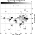
Figure 1: A grayscale plot of the galaxy surface overdensity in the field of the Corona Borealis supercluster for all galaxies brighter than $r=19$ mag in our photometric catalog. The galaxy surface overdensity is the surface density in the supercluster region with the integrated high Galactic latitude counts (to $r=19$ mag) from Weir et al. (1995) subtracted off and then normalized by the subtracted value. The bar on the right side shows the intensity scale. While the Abell clusters stand out prominently, the smoothly distributed component of galaxies in the supercluster is quite weak and may be easily discerned only in the diamond-shaped region defined by A2056, A2065, A2079, A2089.

Figure 1 shows the surface overdensity of galaxies with $r\leq 19$ mag from our photometric catalog in the supercluster field. In order to emphasize the structure of the supercluster, we have subtracted the mean integrated field galaxy counts measured in high Galactic latitude fields by Weir, Djorgovski, & Fayyad (1995) and then divided by this number to obtain the projected surface overdensity. The Abell clusters in the field, including the ones that are more distant than the supercluster, stand out prominently. Four of the Abell clusters (A2056, A2065, A2079, and A2089) are grouped together in the southern part of the supercluster, A2061 and A2067 are close together in the northern part, and A2092 is isolated in the northeastern part. Only in the diamond-shaped region delineated by A2056, A2065, A2079, and A2089 can an extended area with excess galaxy counts be discerned.

In Figure 2, we plot redshift-right-ascension pie diagrams for all galaxies in our survey with $z<0.15$. The diagrams are split by declination as indicated in the figure. The Corona Borealis supercluster is sharply delimited along the line-of-sight by foreground and background underdense regions. The well defined boundaries of the supercluster lead us to restrict our analysis to galaxies with $0.06<z<0.09$. The group of galaxies at $cz\approx 10000$ km s^-1 is part of the “Great Wall” described by Geller & Huchra (1989). The background supercluster at $z\approx 0.11$ is also evident.

The locations on the sky of all survey galaxies for which we have obtained redshifts are plotted in Figure 3. The galaxies marked by large dots have redshifts which place them within the Corona Borealis supercluster ($0.06\leq z\leq 0.09$). The twelve large circles, each of which has a radius of roughly $1h^{-1}$ Mpc, mark the positions of the Abell clusters projected into the field of the supercluster; the seven whose names are underlined are the Abell clusters with redshifts which place them in the supercluster. Seventeen fields, the six at right ascension 15^h13^m, the two southernmost ones at right ascension 15^h17^m, and all nine along the A2061-A2067 ridge, were observed when only a 1024² CCD was available at Palomar, thus reducing the number of usable fibers by a factor of two. The precise positions of the observed fields are listed in Paper I. The total number of galaxies for which redshifts were successfully measured (i.e., including galaxies not in the Corona Borealis supercluster) ranges from 10 to 42 for the fields observed with a 1024² CCD and from 59 to 87 for fields observed with a 2048² CCD. Thus, the Norris fields which contain only a few supercluster galaxies are sparsely populated because the supercluster is truly not dense in those regions. The rapid decline in galaxy density around the A2061-A2067 ridge is particularly striking. A similarly complex and irregular distribution of galaxies has been found in the Shapley supercluster (Quintana et al. 1995).

In order to quantify our visual impressions of the Corona Borealis supercluster, we have computed the fraction of galaxies in the supercluster which belong to the Abell clusters. In addition to the seven catalogued Abell clusters, we also include an additional cluster which we have identified at R.A. $15^{h}29^{m}$, Decl. $+29^{\circ}08^{m}$. We define a galaxy as belonging to an Abell cluster if its projected separation from the nearest Abell cluster on the sky is less than $3h^{-1}$ Mpc (2 Abell radii) and its velocity is less than $3\ \sigma$, where $\sigma$ is the velocity dispersion, different from the nearest Abell cluster’s mean velocity. We compute the volume densities for galaxies in the Corona Borealis supercluster associated and not associated with the Abell clusters using the methods described in Paper II. The Abell clusters occupy 42% of the supercluster volume, and the galaxy volume density within the Abell clusters is $0.57h^{3}$ Mpc^-3. The volume density of galaxies not associated with the Abell clusters is $0.24h^{3}$ Mpc^-3. Thus, approximately two-thirds of the galaxies in the supercluster are associated with one of the Abell clusters. About half of the galaxies have projected separations from the nearest Abell cluster of less than $1.5h^{-1}$ Mpc (1 Abell radius).

The detailed structure of the supercluster, in particular the fact that the component not associated with the Abell clusters accounts for only one-third of the galaxies, is consistent with expectations from both large redshift surveys and theoretical analyses that the supercluster is being constructed from infalling clusters which were formed outside of the supercluster. The largest published redshift survey, the Las Campanas Redshift Survey (Shectman et al. 1996), reveals a web-like pattern in which galaxies lie on filaments and sheets surrounding underdense regions. Clusters and, more rarely, superclusters form at the intersections of the filaments (Doroshkevich et al. 1996). Similar patterns in large-scale structure are revealed in $N$-body cosmological simulations. In addition, theoretical analyses of the merger history of dark matter halos (e.g., Lacey & Cole 1993) indicate that a large halo often forms from the merging of a small number of pieces (which, of course, have themselves formed from even smaller sub-units).

The true geometry of the supercluster, both in the plane of the sky and along the line of sight, is difficult to determine. Bahcall (1992) has marshalled circumstantial evidence to argue that while the region containing the seven Abell clusters is only $\sim 20h^{-1}$ Mpc on a side in the plane of the sky, the entire supercluster extends for at least $\sim 100h^{-1}$ Mpc. First, the far side of the Boötes void, at right ascension $14^{h}30^{m}$, declination $+50^{\circ}$, (Kirshner et al. 1987) is also at a redshift of $z\approx 0.07$. Second, one of the peaks in the redshift distribution of the Broadhurst et al. (1990) pencil-beam survey of the Galactic Poles is at the redshift of the Corona Borealis supercluster, even though the north Galactic Pole is $45^{\circ}$ away from the core of the supercluster. Larger surveys such as the ongoing Center for Astrophysics Century Survey and the planned Sloan survey will presumably be able to delineate the true extent of the supercluster on the plane of the sky.

The core of the supercluster is dramatically elongated along the line of sight in redshift space. However, the elongation in redshift space could in principle be due to a true elongation in real space, to peculiar velocities, or to a combination of both. We represent our uncertainty about the true geometry of the supercluster by the dimensionless parameter $f$, which is the ratio of the redshift-space to real-space elongation of the supercluster. The depth of the supercluster in real space is $\Delta r=(\Delta s/f)h^{-1}$ Mpc, where $\Delta s=c\Delta z/H_{0}$ is the elongation of the supercluster in redshift space. With $\Delta z=0.03$, $\Delta s=90h^{-1}$ Mpc. If the depth along the line of sight is comparable to the diameter of the core of the supercluster on the plane of the sky, $\sim 20h^{-1}$ Mpc, then $f\approx 5$. In contrast, $f\approx 1$ corresponds to the case in which the peculiar velocities are negligible and the elongation of the supercluster in redshift space is similar to the elongation in real space. The evidence described above for the $100h^{-1}$ Mpc extent of the supercluster on the sky, combined with the theoretical expectation that very large structures will collapse into pancakes (Zeldovich 1970), leads us to favor the conclusion that the apparent elongation of the supercluster along the line of sight is mainly due to peculiar velocities. In addition, the large sheets (e.g., the Great Wall, Geller & Huchra 1989) which appear to form the “skeleton” of the galaxy distribution have widths of $5-10h^{-1}$ Mpc (Doroshkevich et al. 1996, Dellantonio, Bothun, & Geller 1996). Since the width of the Corona Borealis supercluster on the plane of the sky is at least $\sim 20h^{-1}$ Mpc, it is unlikely that Corona Borealis is a sheet aligned along our line of sight. To be conservative, the simulated superclusters which we have used to guide our analysis of the Corona Borealis supercluster (see below) are chosen to have overdensities comparable to the lowest possible overdensity of the Corona Borealis supercluster (i.e., when the supercluster really is elongated in real space, $f\approx 1$).

3 $N$-body Simulations of Superclusters

Since superclusters are unrelaxed and contain obvious substructure (e.g., the Abell clusters themselves), a traditional dynamical analysis seems of questionable utility. From dimensional arguments, however, we expect the mass of the system to be proportional to $v^{2}r$, where are $v$ and $r$ are a suitable scale velocity and radius, respectively. We aim to test this expectation by analysing simulated superclusters extracted from large $N$-body cosmological simulations. The simulated superclusters, which are in general quite spatially anisotropic, also enable us to assess the effects of the non-uniform sampling in our observations on our mass estimates.

As first guesses at successful forms for the mass estimator, we have chosen the virial mass estimator and the projected mass estimator. The standard virial mass estimator is given by

$$\hat{M}_{V}={2\sigma_{3D}^{2}\over G}{1\overwithdelims\langle \rangle r}^{-1}\,,$$ (1)

where $\sigma_{3D}$ is the 3-dimensional velocity dispersion of the system and ${\langle 1/r\rangle}^{-1}$ is the mean harmonic radius. For a bound system (and neglecting projection effects), we in fact expect the virial mass estimator never to overestimate the true mass by more than a factor of 2. This statement follows by considering the three cases for the relationship of the kinetic energy, $K=M_{T}\,\sigma_{3D}^{2}/2$, and the potential energy, $W=-GM_{T}^{2}{\langle 1/r\rangle}/2$, for a bound system and the implied relationship between the estimated mass $\hat{M}_{V}$ and the true mass $M_{T}$:

$${\rm case\>1:} {1\over 2}|W|<K<|W|\,, M_{T}<\hat{M}_{V}<2M_{T}$$

$${\rm case\>2:} K={1\over 2}|W|\,, \hat{M}_{V}=M_{T}$$ (2)

$${\rm case\>3:} K<{1\over 2}|W|\,, \hat{M}_{V}<M_{T}$$

Thus, the worst the virial estimator can do for a bound system is to overestimate its mass by a factor of 2, and this occurs only for a marginally bound system with $K=|W|$. When $K<|W|/2$, the virial mass estimator provides a lower limit to the mass of the system. In our $N$-body experiments described below, we find that all 16 candidate superclusters are bound and that the ratio $\hat{M}_{V}/M_{T}$ satisfies the relationship given in equation (3). We will present evidence in § 4 that the Corona Borealis supercluster is bound.

The virial mass may be calculated from observables using

$$\hat{M}_{V}={3\pi\over G}\sigma^{2}{1\overwithdelims\langle \rangle r_{p}}^{-1},$$ (3)

where $\sigma$ is the line-of-sight velocity dispersion and $\langle 1/r_{p}\rangle^{-1}$ is the mean harmonic projected separation,

$${1\overwithdelims\langle \rangle r_{p}}^{-1}={D\over 2}N(N-1)\biggl{(}\sum_{i}\sum_{j<i}{1\over\theta_{ij}}\biggr{)}^{-1},$$ (4)

where $\theta_{ij}$ is the angular separation of galaxies $i$ and $j$, $D$ is the radial distance to the cluster, and $N$ is the total number of galaxies. This estimator for $\langle 1/r_{p}\rangle^{-1}$ is very sensitive to close pairs and is thus quite noisy, especially for systems which have not been uniformly sampled spatially. An alternative estimator of $\langle 1/r_{p}\rangle^{-1}$ which is less sensitive to irregular sampling and close pairs has been introduced by Carlberg et al. (1996). Their “ringwise” harmonic mean radius is defined by,

$${1\overwithdelims\langle \rangle r_{p}}={N(N-1)\over 2}\sum_{i}\sum_{j<i}{2\over\pi(r_{i}+r_{j})}K(k_{ij}),$$ (5)

where $r_{i}$ and $r_{j}$ are the projected radii of objects $i$ and $j$, $K(k)$ is the complete elliptic integral of the first kind in Legendre’s notation (Press et al. 1992), and $k_{ij}^{2}=4r_{i}r_{j}/(r_{i}+r_{j})^{2}$. Although this estimator was originally developed for systems with circular symmetry on the sky, such as galaxy clusters, we find (see below) that this estimator does give less biased values of $\langle 1/r_{p}\rangle^{-1}$ than the straightforward sum in equation (4).

The projected mass estimator (Bahcall & Tremaine 1981) is given by

$$\hat{M}_{P}={f_{\rm PM}\over GN}\sum_{i}v_{zi}^{2}r_{\perp i}\,,$$ (6)

where $v_{z}$ is the velocity in the cluster frame and $r_{\perp}$ is the projected separation from the cluster center. It is designed to give equal weights to particles at all distances (if $v^{2}\propto 1/r$ on the average), but the estimate depends on the mean eccentricity of the orbits parameterized by $f_{\rm PM}$. It can be shown that $f_{\rm PM}=32/\pi$ for isotropic orbits and $64/\pi$ for radial orbits, independent of the mass distribution (Heisler, Tremaine, & Bahcall 1985). We have chosen to use $f_{\rm PM}=32/\pi$ since this yields the smallest masses.

To test our mass estimators, we have examined 16 simulated superclusters drawn from $N$-body simulations of structure formation in both critical- and low-density universes. The models we chose to simulate were the standard cold dark matter (CDM) model ($\Omega_{0}=1$, $h=0.5$) with a normalization of $\sigma_{8}=0.7$ for the rms mass fluctuations in spheres of radius $8\,h^{-1}$ Mpc and a low-density CDM model with $\Omega_{0}=0.3$, a cosmological constant $\Omega_{\Lambda}=0.7$, and $h=0.75$. The low-density model was normalized to the 4-year COBE quadrupole $Q_{\rm rms-PS}=18\,\mu K$ (Gorski et al. 1996); the corresponding $\sigma_{8}$ is 0.84. The gravitational forces in the simulations were computed with a particle-particle particle-mesh (P³M) code (Bertschinger & Gelb 1991). We have performed both large-box simulations (640 Mpc a side) with random Gaussian initial conditions and small-box simulations (160 Mpc a side) which were constrained to produce objects with an overdensity of roughly 5. The comoving Plummer force softening length was 160 kpc for all simulations. The properties of our entire suite of simulated superclusters are summarized in Table 1, in which we list the identification number of the simulated supercluster, the cosmological model, the comoving box size, the total number of particles in the simulation, the number of particles in the supercluster, the mass of the supercluster, the volume of the region containing the supercluster, the overdensity of the supercluster, and the ratio $2K/|W|$.

To select candidate superclusters from the simulations, we have searched for clustered regions that consist of multiple dark matter halos which have not yet merged into one dominant halo. Overdense regions which violate this criterion would clearly conflict with the observations described here and with those of Quintana et al. (1995) of the Shapley supercluster. In order to test the case in which the Corona Borealis supercluster is the least dynamically evolved, we have chosen regions that have an overdensity of $\sim 5$ in a volume of $30^{3}$ Mpc³. This corresponds to the smallest possible density contrast of the Corona Borealis supercluster, where its elongation in redshift space is mostly due to physical extension along the line of sight in real space (i.e., $f\approx 1$). As we discussed earlier, however, peculiar velocities are likely to have an important effect, and the Corona Borealis supercluster is likely to be more compact in real space than in redshift space ($f>1$) and thus have an overdensity as high as about 40. We expect the mass estimators to work better in this case since the supercluster would then be closer to virialization, which occurs at an overdensity of $\sim 200$. Tests of the mass estimators on smaller regions of our simulated superclusters with overdensities of $\sim 40$ have verified these expectations. It is also important to note that the fractions of particles inside and outside clusters with masses greater than $10^{14}h^{-1}$ $M_{\odot}$ are typically 2/3 and 1/3, respectively, similar to the observed fractions of galaxies inside and outside the Abell clusters within the Corona Borealis supercluster. In Figure 4, we plot the $x$, $y$, and $z$ projections of supercluster #1 to illustrate the type of objects which we have identified as superclusters in the simulations.

In Figure 5, we plot $\hat{M}_{V}/M_{T}$ (filled squares) and $\hat{M}_{P}/M_{T}$ (unfilled squares) as a function of $2K/|W|$ for the $x$, $y$, and $z$ projections of the eight simulated superclusters drawn from $\Omega_{0}=1$ simulations (panel $a$) and of the eight simulated superclusters drawn from $\Omega_{0}=0.3$, $\Omega_{\Lambda}=0.7$ simulations (panel $b$). We also plot the data shown in Figure 5 as histograms in Figure 6 (panels $a$ and $c$). The correlation between $\hat{M}_{V}/M_{T}$ and $2K/|W|$ expected from equation (3) is clearly evident in both panels of Figure 5. For the eight $\Omega_{0}=1$ simulated superclusters, $\langle\hat{M}_{V}/M_{T}\rangle=0.94\pm 0.24$ and $\langle\hat{M}_{P}/M_{T}\rangle=0.76\pm 0.24$, where the averages are over the three projections of the eight simulated superclusters. The excellent accuracy of the virial mass estimator reflects the fact that the mean and dispersion about the mean of $2K/|W|$ for these eight simulated superclusters are 0.96 and 0.14, respectively. We have also examined eight simulated superclusters drawn from the low-density simulations in order to test the sensitivities of the mass estimators to cosmology. Here, too, the virial mass estimator gives more accurate results than the projected mass estimator: $\langle\hat{M}_{V}/M_{T}\rangle=0.99\pm 0.21$ and $\langle\hat{M}_{P}/M_{T}\rangle=1.04\pm 0.52$. Note, however, that the projected mass estimator gives large overestimates of the true mass for superclusters #14 and #15, which is due to the fact that both superclusters have large fractions of their mass at large radii. When values of $\hat{M}_{P}/M_{T}$ larger than 1.5 are excluded, then $\langle\hat{M}_{P}/M_{T}\rangle=0.78\pm 0.24$, which is in line with the result previously obtained for the simulated superclusters extracted from the $\Omega_{0}=1$ simulations. We conclude that the virial mass estimator provides robust estimates of the masses of superclusters and is insensitive to $\Omega_{0}$. The projected mass estimator is less accurate and can lead to substantial overestimates, as much as a factor of two, for superclusters with unusually large amounts of mass at large radii.

The tests above used all the simulation particles in each supercluster. Our observations, however, do not sample every galaxy in the supercluster. We have therefore performed simulated observations of the simulated superclusters to estimate the effects of irregular sampling in our redshift survey. For each simulated supercluster, we projected the supercluster along an axis and chose only those particles which lie in 16 randomly-positioned fields. The total area covered by the 16 fields was 10% of the total projected area of the supercluster, matching the fraction of the area of the Corona Borealis supercluster which we surveyed. A fraction of the particles in each field were randomly rejected so that the total number of particles used in the simulated observations was roughly 500, comparable to the number of galaxies with measured redshifts in Corona Borealis. The results of our simulated observations are summarized in Table 2, in which we record for each supercluster the masses (relative to the true mass) found by the virial mass estimator and the projected mass estimator for the $x$, $y$, and $z$ projections. We also plot the results of our simulated observations as histograms in Figure 6 (panels $b$ and $d$). The non-uniform sampling of the simulated observations tends to reduce the masses estimated with the virial mass estimator, mainly due to a systematic underestimate of $\langle 1/r_{p}\rangle^{-1}$. The non-uniform sampling does not significantly affect estimates of the velocity dispersion. For the $\Omega_{0}=1$ models, the virial mass estimator underestimates the true mass by 31%, and the projected mass estimator underestimates the true mass by 21%. For the low-density models, the virial mass estimator underestimates the true mass by 5%, and the projected mass estimator overestimates the true mass by 27%. The dispersion around these values is $\sim 20-25$%. It is clear that the “ringwise” estimator of the projected mean harmonic radius is not completely correcting for our non-uniform sampling, which is to be expected since the estimator is designed for systems with circular symmetry on the sky. Nevertheless, the “ringwise” estimator does improve the accuracy of our mass estimates by 20% relative to mass estimates using the conventional mean harmonic projected separation given by equation (4). These results indicate that both the virial mass estimator and the projected mass estimator can be reliably applied to superclusters, despite the fact that superclusters are clearly not in equilibrium. With our irregular sampling, the estimators generally underestimate the true mass of the system.

Although the circumstantial evidence suggests that the Corona Borealis supercluster extends for $\sim 100h^{-1}$ Mpc on the sky (§ 2), it is still important to consider the possibility that the Corona Borealis supercluster has an extreme prolate shape in which we are looking along the long axis. Our simulated supercluster #1 has a fairly linear geometry with most of the mass concentrated along a chain of structures. By observing along this chain, we can assess how accurately the mass estimators will estimate the true mass in the pathological case in which the Corona Borealis supercluster is a cigar-shaped structure pointed directly at us. For the simulated supercluster #1, the virial mass and projected estimators underestimate the mass of the supercluster by 50% when the supercluster is observed along its axis, due, in roughly equal importance, to reductions in the velocity dispersion and $\langle 1/r_{p}\rangle^{-1}$. The reduction of the velocity dispersion is caused by coherent infall along the supercluster’s axis. Thus, if the Corona Borealis supercluster is a prolate structure pointed directly at us, it is likely we will underestimate its mass.

4 The Dynamics and Mass of the Corona Borealis Supercluster

We demonstrated in the previous section that the virial and projected mass estimators can be reliably applied to simulated superclusters that resemble the Corona Borealis supercluster. Before doing so, however, we present general considerations of the dynamical state of the supercluster using the evolution of a spherical overdensity in an expanding universe as our model (Peebles 1980). The supercluster is certainly not perfectly spherical, and our knowledge of the structure along the line of sight is particularly unconstrained (§2). However, the models of Eisenstein & Loeb (1995) illustrate that the turn-around times of the short axes of a triaxial perturbation are fairly well predicted by the turn-around time of a spherical perturbation with the same initial density and that the overdensity inside the triaxial perturbation is well described by the spherical model to overdensities of $\sim 50$.

The galaxy number overdensity of the supercluster for $M(B_{AB})\leq-16.3+5\log h$ mag is $\delta_{SC}=(n_{SC}/\bar{n})-1\approx 7f$, where $n_{SC}$ and $\bar{n}$ are the mean number densities of galaxies in the supercluster and in the field, respectively, and $f$, introduced in §2, is the ratio of the redshift-space to real-space elongation along the line of sight. An outer shell of a density perturbation is bound if the mean overdensity within the shell is greater than $(\Omega_{0}^{-1}-1)/(1+z)$. There is only a very small range of positive density perturbations that are not bound (i.e., $0<\delta<(\Omega_{0}^{-1}-1)/(1+z)$), and it is thus unlikely to observe a supercluster with an appreciable density contrast which is freely expanding. Taking $\Omega_{0}=0.3$ as a very rough lower limit on the density parameter, the overdensity of the supercluster must be greater than 2.1 for the supercluster to be bound. The supercluster is, then, clearly bound. While bound, the supercluster could still be expanding and yet to turn around. The overdensity required for turn-around has been computed for $\Omega_{0}\leq 1$ by Silk (1977) and by Regős & Geller (1989). For $\Omega_{0}=1$, the turn-around overdensity is the well-known value $(9\pi^{2}/16)-1\approx 4.55$. For $\Omega_{0}=0.3$, the turn-around overdensity is $\approx 12$. From Figure 4 of Regős & Geller (1989), we see that the supercluster is likely to be collapsing unless the supercluster is quite elongated in real space ($f\lesssim 2$) and $\Omega_{0}\lesssim 0.4$.

Before we compute the mass of the whole supercluster, we recompute the lower limit to the mass of the supercluster determined by simply adding up the masses of the individual Abell clusters. For each of the eight clusters (the seven catalogued clusters plus the cluster which we have identified at R.A. $15^{h}29.2^{m}$, Decl. $+29^{\circ}08^{m}$), we identify all galaxies within a projected distance of $1.5h^{-1}$ Mpc (1 Abell radius) of the cluster center and compute the cluster mass with the virial mass estimator (using the ringwise harmonic mean projected radius). We do not have redshifts for enough galaxies in Abell 2056 to estimate reliably its mass. The other clusters are, however, well sampled, ranging from 26 redshifts in Abell 2079 to 105 in Abell 2061. We use the biweight estimators and bias-corrected, bootstrap errors for our determinations of the centroid velocities and dispersions and their associated errors, as recommended by Beers, Flynn, & Gebhardt (1990). The velocity dispersions are corrected to the cluster rest frames. The results for the individual clusters are summarized in Table 3, where we record for each cluster its centroid velocity, dispersion, harmonic mean projected radius, and virial mass. The quoted errors are 90% confidence intervals. The sum of the masses of the seven clusters for which we have adequate data is $5.3\times 10^{15}h^{-1}M_{\odot}$, a factor of 2 larger than the sum computed by Postman et al. (1988). This difference is mainly due to the fact that we computed the masses within a projected radius of $1.5h^{-1}$ Mpc, whereas Postman et al. (1988) used $1.0h^{-1}$ Mpc. Our sum is also based on seven rather than six clusters.

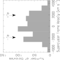
Figure 7: Line-of-sight velocity histogram for the Corona Borealis supercluster in the supercluster frame. We have marked $\pm 1\sigma$, where $\sigma$ is the velocity dispersion, with arrows. The mean recession velocity of the supercluster is $22420^{+149}_{-138}$ km s^-1, and $\sigma=1929^{+81}_{-67}$ km s^-1.

We have plotted the line-of-sight velocity histogram (in the supercluster frame) for the Corona Borealis supercluster in Figure 7. Again using the techniques of Beers, Flynn, & Gebhardt (1990), we estimate the centroid velocity of the Corona Borealis supercluster to be $c\bar{z}=22420^{+149}_{-138}$ km s^-1 and the dispersion to be $\sigma=1929^{+81}_{-67}$ km s^-1 in the cluster rest frame. The errors bars are 90% confidence intervals. Due to our irregular sampling of the supercluster, which itself has an irregular density distribution, it is not straightforward to estimate the harmonic mean projected radius. We have taken two approaches. First, we have used the “ringwise” estimator described by Carlberg et al. (1996), which yields $\langle 1/r_{p}\rangle^{-1}=4.6h^{-1}$ Mpc. Second, we have estimated $\langle 1/r_{p}\rangle^{-1}$ using all the galaxies in the supercluster field with $16\ {\rm mag}\leq r\leq 19\ {\rm mag}$, whether or not they have measured redshifts, weighted by the observed redshift distribution as a function of $r$ magnitude. This method yields $\langle 1/r_{p}\rangle^{-1}=4.1h^{-1}$ Mpc, 11% smaller than the value obtained using the “ringwise” estimator. The virial mass estimator gives a mass for the Corona Borealis supercluster of $3.8\times 10^{16}h^{-1}$ $M_{\odot}$ using $\langle 1/r_{p}\rangle^{-1}=4.6h^{-1}$ Mpc and $3.3\times 10^{16}h^{-1}$ $M_{\odot}$ using $\langle 1/r_{p}\rangle^{-1}=4.1h^{-1}$ Mpc. The projected mass estimator yields a similar value, $4.2\times 10^{16}h^{-1}$ $M_{\odot}$. If we apply the two mass estimators to the eight clusters, treated as test particles, we also obtain values for the total mass of the supercluster of $4\times 10^{16}h^{-1}$ $M_{\odot}$. While case 3 of equation (3) demonstrates that the virial theorem can in principle underestimate the mass of a bound system by an arbitrarily large amount, the results of our simulations, which are recorded in Table 2 and depicted in Figure 6, indicate that we are unlikely to underestimate the mass of the Corona Borealis supercluster by more than a factor of 2. We thus place a rough upper limit on the mass of the supercluster of $8\times 10^{16}h^{-1}$ $M_{\odot}$, comparable to the upper limit derived by Postman et al. (1988).

Given the results of our tests of the virial mass estimator and the projected mass estimator on simulated superclusters described in § 3, we believe that a secure lower bound to the mass of the Corona Borealis supercluster is $3\times 10^{16}h^{-1}$ $M_{\odot}$. By integrating the supercluster luminosity function, we can compute the mean luminosity density of the supercluster and thereby measure the $M/L$ ratio of the supercluster on scales of $\sim 20h^{-1}$ Mpc. The supercluster luminosity function for $M(B_{AB})\leq-16.3+5\log h$ mag, where we are using the AB-normalized $B$ band (Oke 1974), is presented in Paper II; a straightforward integration of the luminosity function yields a mean luminosity density in the supercluster in the $B_{AB}$ band of $\rho_{L}(B_{AB})=1.9\times 10^{9}hL_{\odot}$Mpc^-3. Taking the solid angle of the survey to be 0.0076 sr (= 25 deg²) and the limits of the supercluster to be at $z=0.06$ and $z=0.09$, the volume of the region surveyed is $2.8\times 10^{4}h^{-3}$ Mpc³. The $M/L$ ratio of the supercluster in the $B_{AB}$ band is thus $564h{M\overwithdelims( )L}_{\sun}$. Our mass estimates for the Corona Borealis supercluster are comparable to the mass estimates derived by Postman et al. (1988) under the assumption that the differences in the mean redshifts of the constituent clusters are due to peculiar motions generated by the supercluster. Their best estimate of the supercluster mass is, however, five times smaller than ours because they assumed that the $M/L$ ratio of the Corona Borealis supercluster was similar to that of rich clusters and they used a supercluster volume only one-third the size of the volume we used.

We can repeat our analysis of the Corona Borealis supercluster on the background A2069 supercluster. From inspection of Figure 2, we take the redshift limits of the A2069 supercluster to be $z=0.10$ and $z=0.13$, which gives us 352 galaxies with measured redshifts in the supercluster. The galaxy number overdensity of the A2069 supercluster between these redshift limits and for $M(B_{AB})\leq-17.5+5\log h$ mag is $\delta_{SC}\approx 4f_{A2069}$, where we again parameterize the depth of the supercluster along the line of sight in real space as $\Delta r=(\Delta s/f_{A2069})$ Mpc, with $\Delta s=c\Delta z/H_{0}=90h^{-1}$ Mpc for $\Delta z=0.03$. The minimum overdensity is obtained for $f_{A2069}\approx 1$, which corresponds to the case in which the peculiar velocities are negligible and the elongation in redshift space is similar to the elongation in real space. If, on the other hand, the depth in real space is similar to the diameter of the supercluster in the plane of the sky, then $f_{A2026}\approx 5$. For $\Omega_{0}=0.3$ and $z=0.115$, a spherical perturbation with an overdensity of $(\Omega_{0}^{-1}-1)/(1+z)\approx 2.1$ is bound. Thus, the A2069 supercluster is likely to bound, although possibly only marginally so if $f_{A2069}\approx 1$. If the supercluster is, indeed, only marginally bound, then we would expect, in light of the discussion in §3, that the virial mass estimator may overestimate the mass of the supercluster, but by no more than a factor of 2.

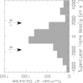
Figure 8: Line-of-sight velocity histogram for the A2069 supercluster in the supercluster frame. We have marked $\pm 1\sigma$, where $\sigma$ is the velocity dispersion, with arrows. The mean recession velocity of the supercluster is $34338^{+148}_{-140}$ km s^-1, and $\sigma=1684^{+145}_{-151}$ km s^-1.

The centroid velocity and velocity dispersion of the A2069 supercluster are $34338^{+148}_{-140}$ km s^-1 and $1684^{+145}_{-151}$ km s^-1, respectively. We have plotted the line-of-sight velocity histogram (in the supercluster frame) of the A2069 supercluster in Figure 8. As for our analysis of the Corona Borealis supercluster, we take two approaches to estimating the mean harmonic projected radius. The Carlberg et al. (1996) “ringwise” estimator yields $\langle 1/r_{p}\rangle^{-1}=6.5h^{-1}$ Mpc. We have also estimated the mean harmonic projected radius using all galaxies with $16\leq r\leq 19$ in the supercluster field, corrected by the measured redshift distribution as a function of magnitude. This procedure gives $\langle 1/r_{p}\rangle^{-1}=5.2h^{-1}$ Mpc, a 20% reduction from the value obtained with the “ringwise” estimator. Using the virial mass estimator, the mass of the A2069 supercluster is $4.1\times 10^{16}h^{-1}$ $M_{\odot}$ with the larger value of $\langle 1/r_{p}\rangle^{-1}$ or $3.3\times 10^{16}h^{-1}$ $M_{\odot}$ with the smaller value. With the projected mass estimator, the mass of the A2069 supercluster is $6\times 10^{16}h^{-1}M_{\odot}$. A firm lower limit to the mass of the A2069 supercluster is, therefore, $3\times 10^{16}h^{-1}$ $M_{\odot}$. Integrating the A2069 supercluster luminosity function, we find that the luminosity density of the A2069 supercluster is $\rho_{L}(B_{AB})=7.0\times 10^{8}hL_{\odot}$Mpc^-3. We surveyed $5.9\times 10^{4}h^{-3}$ Mpc³ in the A2069 supercluster, and we thus find that the $M/L$ ratio of the A2069 supercluster in the $B_{AB}$ band, using the lower limit mass of $3\times 10^{16}h^{-1}$ $M_{\odot}$, is $726h{M\overwithdelims( )L}_{\odot}$, roughly 30% higher that the $M/L$ ratio of the Corona Borealis supercluster. 10% of the difference is due to the brighter integration limit for the luminosity density of the A2069 supercluster. The remaining 20% difference between the two superclusters is not, however, likely to be significant, given both the $\sim 25$% error in the mass estimators and the possibility that the mass estimators will tend to overestimate modestly the true mass of a weakly bound system such as the A2069 supercluster.

5 Discussion

As an immediate application of our measurement of the $M/L$ ratio of the Corona Borealis and A2069 superclusters, we can estimate $\Omega_{0}$ on a scale of $\sim 20h^{-1}$ Mpc by comparing the $M/L$ ratio of the superclusters to the $M/L$ ratio required to close the universe. As computed from our determination of the local luminosity function (Paper II), the $B_{AB}$-band luminosity density for galaxies with $M(B_{AB})\leq-16.3+5\log h$ mag is $1.8\times 10^{8}L_{\odot}h$ Mpc^-3. The uncertainty in this number is dominated by systematic errors, and so the most straightforward means to assess the uncertainty is simply to compare values obtained in independent redshift surveys of local galaxies. The largest local survey is the Las Campanas Redshift Survey (Shectman et al. 1996). The luminosity function from this survey has been computed by Lin et al. (1996) and yields a luminosity density in the $B_{AB}$-band of $1.6\times 10^{8}L_{\odot}h$ Mpc^-3, where we have used $\langle B_{AB}-r_{\rm LCRS}\rangle=0.72$ mag to convert from isophotal hybrid $r_{\rm LCRS}$ magnitudes to total $B_{AB}$ magnitudes (see Paper II) and we have assumed a flat slope for the low luminosity end of the luminosity function. The luminosity density for $M(B_{AB})<-16+5\log h$ mag reported by Zucca et al. (1997) for the ESO Slice Project is $2.0\times 10^{8}L_{\odot}h$ Mpc^-3. Finally, the luminosity densities obtained by integrating the local luminosity functions measured by Ellis et al. (1996) from the Autofib Survey and Ratcliffe et al. (1997) from the Durham/UKST Galaxy Redshift Survey are $1.9\times 10^{8}L_{\odot}h$ Mpc^-3 and $1.7\times 10^{8}L_{\odot}h$ Mpc^-3 in the $B_{AB}$ band, respectively. Thus, we conclude that the local $B_{AB}$-band luminosity density is $(1.8\pm 0.2)\times 10^{8}L_{\odot}h$ Mpc^-3 for $M(B_{AB})\lesssim-16+5\log h$ mag. The corresponding critical $M/L$ ratio to close the universe is $1550\pm 170h{M\overwithdelims( )L}_{\odot}$.

The final step before deriving a value for $\Omega_{0}$ is to consider whether there has been differential luminosity evolution between galaxies in the superclusters and in the field. There is no reason, in principle, why the luminosity per unit mass in the superclusters should be identical to that in the field. However, Carlberg et al. (1997) report that galaxies in the cores of rich clusters have only faded by 0.11 mag relative to galaxies in the field, and so we expect a very small variation between the galaxies in the superclusters, which are on average significantly less dense than rich clusters, and the galaxies in the field. In Paper II, we compared the luminosity functions of the Corona Borealis and A2069 superclusters to the local field luminosity function. We found that the characteristic luminosity, $L^{\ast}$, was $\sim 0.5$ mag brighter in the Corona Borealis supercluster than in the field, while $L^{\ast}$ in the A2069 supercluster was very close to the value in the field. Since the measured value of $L^{\ast}$ is strongly correlated with the poorly-constrainted faint end slope of the luminosity function, the errors on $L^{\ast}$ are quite large ($\gtrsim 0.3$ mag). Nevertheless, there is no evidence for fading of supercluster galaxies relative to field galaxies; any correction for brightening of supercluster galaxies relative to field galaxies would raise our estimate of $\Omega_{0}$.

The $M/L$ ratio of the Corona Borealis supercluster is $564h{M\overwithdelims( )L}_{\odot}$, and therefore we determine that $\Omega_{0}=0.36$ on supercluster scales, or roughly twice the value computed by Carlberg et al. (1996) for rich clusters of galaxies. Repeating the above analysis for the A2069 supercluster, but only computing the luminosity densities for $M(B_{AB})\leq-17.5+5\log h$ mag, gives $\Omega_{0}=0.44$. Since our simulated observations of our simulated superclusters indicate that our mass estimators are likely to underestimate (by $\lesssim 30\%$) the true masses of the superclusters, we conclude that $\Omega_{0}\gtrsim 0.4$ on $\sim 20h^{-1}$ Mpc scales, which is comparable to estimates of $\Omega_{0}$ on similar and larger scales based on analyses of large-scale velocity flows (Strauss & Willick 1995) and agrees with the “tentative consensus” value reached by Dekel et al. (1996).

The principal weakness of our measurement of $\Omega_{0}$ is, of course, that it is based on only two superclusters. However, future large-area redshift surveys should generate data for a much larger number of superclusters. In particular, the imminent 2dF (Colless 1997) and Sloan surveys will densely map substantial fractions of the sky and provide large numbers of redshifts for many superclusters.

Table 1: Properties of the Simulated Superclusters

ID #	Model	Box	$N_{tot}$	$N_{SC}$	MSC	VSC	${\delta\rho\over\rho}$	$2K/|W|$
		($h^{-1}$ Mpc)			($10^{15}h^{-1}$ $M_{\odot}$)	($10^{3}h^{-3}$ Mpc3)
1	CDM	320	$256^{3}$	9780	5.3	3.4	4.7	0.98
2	CDM	320	$256^{3}$	9657	5.3	3.4	4.6	1.07
3	CDM	320	$256^{3}$	10089	5.5	3.7	4.4	0.89
4	CDM	320	$256^{3}$	9684	5.3	3.7	4.1	0.84
5	CDM	80	$64^{3}$	9694	5.3	3.4	4.6	0.85
6	CDM	80	$64^{3}$	13890	7.6	3.4	7.0	1.23
7	CDM	80	$64^{3}$	10755	5.9	3.4	5.2	1.06
8	CDM	80	$64^{3}$	8619	4.7	3.4	4.0	0.79
9	$\Lambda$CDM	480	$128^{3}$	1265	5.6	11.4	4.9	0.98
10	$\Lambda$CDM	480	$128^{3}$	1261	5.6	11.4	4.8	1.08
11	$\Lambda$CDM	480	$128^{3}$	1390	6.1	12.3	4.9	0.85
12	$\Lambda$CDM	480	$128^{3}$	1261	5.6	12.5	4.3	0.83
13	$\Lambda$CDM	120	$64^{3}$	8251	4.6	11.4	3.8	0.84
14	$\Lambda$CDM	120	$64^{3}$	8631	4.8	11.2	4.1	1.23
15	$\Lambda$CDM	120	$64^{3}$	11477	6.3	11.4	5.6	1.20
16	$\Lambda$CDM	120	$64^{3}$	11483	6.3	11.4	5.6	1.07

Table 2: Mass Estimates for the Simulated Superclusters from Simulated Observations

ID #	x-axis		y-axis		z-axis
	${\hat{M}_{V}\over M_{T}}$	${\hat{M}_{P}\over M_{T}}$	${\hat{M}_{V}\over M_{T}}$	${\hat{M}_{P}\over M_{T}}$	${\hat{M}_{V}\over M_{T}}$	${\hat{M}_{P}\over M_{T}}$
1	$0.61\pm 0.20$	$0.76\pm 0.23$	$0.59\pm 0.18$	$0.66\pm 0.19$	$0.99\pm 0.36$	$1.13\pm 0.41$
2	$0.67\pm 0.21$	$0.74\pm 0.19$	$0.64\pm 0.21$	$0.63\pm 0.18$	$0.81\pm 0.25$	$0.84\pm 0.25$
3	$0.82\pm 0.24$	$0.87\pm 0.23$	$0.55\pm 0.17$	$0.59\pm 0.17$	$0.55\pm 0.25$	$0.64\pm 0.26$
4	$0.71\pm 0.20$	$0.84\pm 0.25$	$0.65\pm 0.25$	$0.83\pm 0.35$	$0.45\pm 0.12$	$0.56\pm 0.16$
5	$0.78\pm 0.26$	$1.07\pm 0.33$	$0.67\pm 0.26$	$0.87\pm 0.36$	$0.87\pm 0.30$	$1.09\pm 0.41$
6	$1.15\pm 0.48$	$1.40\pm 0.58$	$0.60\pm 0.19$	$0.71\pm 0.25$	$0.59\pm 0.20$	$0.66\pm 0.24$
7	$0.63\pm 0.16$	$0.65\pm 0.14$	$0.52\pm 0.17$	$0.51\pm 0.14$	$0.87\pm 0.27$	$0.93\pm 0.24$
8	$0.42\pm 0.13$	$0.45\pm 0.14$	$0.67\pm 0.13$	$0.76\pm 0.17$	$0.68\pm 0.24$	$0.76\pm 0.25$
13	$0.54\pm 0.29$	$0.73\pm 0.39$	$0.82\pm 0.27$	$1.01\pm 0.35$	$0.79\pm 0.34$	$1.12\pm 0.45$
14	$1.23\pm 0.46$	$1.65\pm 0.58$	$1.42\pm 0.55$	$1.96\pm 0.73$	$1.00\pm 0.36$	$1.34\pm 0.47$
15	$1.12\pm 0.58$	$1.55\pm 0.82$	$0.91\pm 0.40$	$1.29\pm 0.51$	$1.09\pm 0.54$	$1.41\pm 0.73$
16	$0.79\pm 0.22$	$1.00\pm 0.28$	$0.67\pm 0.36$	$0.86\pm 0.43$	$1.06\pm 0.31$	$1.33\pm 0.37$

Note. — Because superclusters #9, #10, #11, and #12 were drawn from a simulation with a large box size ($640^{3}$ Mpc³) but with a comparatively small number of particles ($128^{3}$), simulated observations of 10% of the area yield only $\sim 120$ particles, and so we have excluded these superclusters from our analysis of simulated observations.

Table 3: Galaxy Clusters in the Corona Borealis Supercluster

Cluster	$N_{z}$	Centroid	Dispersion	${1\overwithdelims\langle \rangle r_{p}}^{-1}$	$M_{V}$
		km s-1	km s-1	$h^{-1}$ Mpc	$10^{14}h^{-1}$ $M_{\odot}$
A2056	10	$\cdots$	$\cdots$	$\cdots$	$\cdots$
A2061	105	$23512^{+170}_{-143}$	$1020^{+180}_{-182}$	0.40	$9.08^{+3.49}_{-2.95}$
A2065	31	$21767^{+369}_{-367}$	$1203^{+371}_{-289}$	0.58	$18.5^{+13.2}_{-8.2}$
A2067	55	$22435^{+280}_{-220}$	$953^{+175}_{-250}$	0.56	$11.1^{+4.5}_{-5.1}$
A2079	26	$19656^{+209}_{-239}$	$652^{+295}_{-172}$	0.62	$5.82^{+6.48}_{-2.67}$
A2089	30	$21968^{+136}_{-185}$	$545^{+246}_{-207}$	0.73	$4.77^{+5.28}_{-2.94}$
A2092	44	$20064^{+137}_{-124}$	$581^{+252}_{-138}$	0.27	$1.99^{+2.10}_{-0.83}$
Cl1529+29	43	$25145^{+162}_{-195}$	$534^{+92}_{-80}$	0.29	$1.82^{+0.68}_{-0.50}$

Figure 2: Redshift-right-ascension cone diagrams for galaxies in our survey with $cz<45000$ km s^-1, divided into 3 declination slices. The Corona Borealis supercluster is the prominent overdense region between $cz\approx 18000$ km s^-1 and $cz\approx 27000$ km s^-1; these limits are marked in the cone diagrams by the heavy lines. The dashed lines mark the background supercluster at $cz\approx 34000$ km s^-1. The smaller structure at $cz\approx 10000$ km s^-1 is part of the “Great Wall” of galaxies.

Figure 3: Location on the sky of galaxies with measured redshifts in the field of the Corona Borealis supercluster. The galaxies marked with large dots are galaxies with redshifts placing them within the supercluster ($0.06\leq z\leq 0.09$). The twelve large circles, whose radii are roughly $1h^{-1}$ Mpc, mark the positions of the twelve Abell clusters in the field. The clusters whose names are underlined are contained in the Corona Borealis supercluster. The number of galaxies successfully identified at all redshifts ranges from 10 to 42 for fields observed when only half of the Norris Spectrograph’s fibers were usable because a large format 2048² CCD was not yet available at Palomar, and from 59 to 87 for fields observed with the large format 2048² CCD. The precise locations of the observed fields are given in Paper I.

Figure 4: $x$, $y$, and $z$ projections of our simulated supercluster #1. Note in the $z$ projection the relatively linear, chain-like structure. To simulate observing along the long axis of a cigar-shaped supercluster, we rotate the supercluster in the $x$-$y$ plane by $45^{\circ}$ clockwise and then observe along the $y$-axis.

Figure 5: Ratio of the mass estimated with the virial mass estimator (filled squares) or the projected mass estimator (unfilled squares) to the true mass, as a function of $2K/|W|$ for our simulated superclusters. Results from superclusters drawn from $\Omega_{0}=1$ simulations are plotted in panel $(a)$, while results from superclusters from $\Omega_{0}=1$, $\Omega_{\Lambda}=0.7$ simulations are plotted in panel $(b)$. $\hat{M}_{V}/M_{T}$ is correlated with $2K/|W|$ as one would expect from equation (3). The projected mass estimator can substantially overestimate the mass of a supercluster with only a very small central concentration of mass and a large amount of mass at large radii.

Figure 6: Histograms of $\hat{M}_{V}/M_{T}$ (thick line) and $\hat{M}_{P}/M_{T}$ (thin line). The histograms shown in panels $(a)$ and $(c)$ are based on mass estimates using all of the simulation particles, while the histograms shown in panels $(b)$ and $(d)$ are based on mass estimates from the simulated observations. The results for the superclusters drawn from the $\Omega_{0}=1$ simulations are given in panels $(a)$ and $(b)$, and the results for the superclusters drawn from the $\Omega_{0}=0.3$, $\Omega_{\Lambda}=0.7$ simulations are given in panels $(c)$ and $(d)$. Each observation is an observation along the $x$, $y$, or $z$ axis of one of the superclusters. The results for only four superclusters are plotted in panel $(d)$; see the note to Table 2. The sparse and irregular sampling of the simulated observations causes at most $\sim 30\%$ reductions in the accuracies of both the virial mass estimator and the projected mass estimator.

References

- Abell (1958) Abell, G. 1958, ApJS, 3, 211
- Bahcall & Tremaine (1981) Bahcall, J., & Tremaine, S. 1981, ApJ, 244, 805
- Bahcall (1992) Bahcall, N. 1992 in Clusters and Superclusters of Galaxies, ed. A. Fabian (Dordrecht: Kluwer), 275
- Bahcall et al. (1995) Bahcall, N., Lubin, L., & Dorman, V. 1995, ApJ, 447, L81
- Beers, Flynn, & Gebhardt (1990) Beers, T., Flynn, K., & Gebhardt, K. 1990, AJ, 100, 32
- Bertschinger & Gelb (1991) Bertschinger, E., & Gelb, J. 1991, Computers in Physics, 5, 164
- Broadhurst et al. (1990) Broadhurst, T., Ellis, R., Koo, D., & Szalay, A. 1990, Nature, 343, 726
- Carlberg et al. (1996) Carlberg, R., Yee, H., Ellingson, E., Abraham, R., Gravel, P., Morris, S., & Pritchet, C. 1996, ApJ, 462, 32
- Carlberg et al. (1997) Carlberg, R., Yee, H., & Ellingson, E. 1997, ApJ, 478, 462
- Colless (1996) Colless, M. 1997, in Wide-Field Spectroscopy, eds. M. Kontizas & E. Kontizas (Dordrecht: Kluwer), in press (astro-ph/9607176)
- Dell’Antonio et al. (1996) Dell’Antonio, I., Bothun, G., & Geller, M. 1996, AJ, 112, 1780
- Doroshkevitch et al. (1996) Doroshkevitch, A., Tucker, D., Oemler, A., Kirshner, R., Lin, H., Shectman, S., Landy, S., & Fong, R. 1996, MN, 283, 1281
- (13) Eisenstein, D. & Loeb, A. 1995, ApJ, 439, 520
- Ellis et al. (1996) Ellis, R., Colless, M., Broadhurst, T., Heyl, J., & Glazebrook, K. 1996, MNRAS, 280, 235
- Ettori et al. (1997) Ettori, S., Fabian, A., & White, D. 1997, MN, in press (astro-ph/9704092)
- Faber & Gallagher (1979) Faber, S. & Gallagher, J. 1979, ARA&A, 17, 135
- Geller & Huchra (1989) Geller, M. & Huchra, J. 1989, Science, 246, 897
- Gorski et al. (1996) Gorski, K. et al. 1996, ApJ, 464, L11
- Gunn (1978) Gunn, J. 1978, in Observational Cosmology, ed. A. Maeder, L. Martinet, & G. Tammann (Sauverny: Geneva Obs.), 1
- Heisler et al. (1985) Heisler, J., Tremaine, S., & Bahcall, J. 1985, ApJ, 298, 8
- Kaiser & Davis (1985) Kaiser, N., & Davis, M. 1985, ApJ, 297, 365
- Kent & Gunn (1982) Kent, S. & Gunn, J. 1982, AJ, 87, 945
- Kent & Sargent (1983) Kent, S. & Sargent, W. 1983, AJ, 88, 697
- Kirshner et al. (1987) Kirshner, R., Oemler, A., Schechter, P., & Shectman, S. 1987, ApJ, 314, 493
- Lacey & Cool (1993) Lacey, C. & Cole, S. 1993, MN, 262, 627
- Lin et al (1996) Lin, H., Kirshner, R., Shectman, S., Landy, S., Oemler, A., Tucker, D., & Schechter, P. 1996, ApJ, 464, 60
- Mohr et al. (1996) Mohr, J., Geller, M., & Wegner, G. 1996, AJ, 112, 1816
- Oke (1974) Oke, J. 1974, ApJS, 27, 21
- Peebles (1980) Peebles, P. 1980, The Large-Scale Structure of the Universe (Princeton: Princeton University Press)
- Picard (1991) Picard, A. 1991, AJ, 102, 445
- Postman et al. (1986) Postman, M., Geller, M., & Huchra, J. 1986, AJ, 91, 6
- Postman, Geller, & Huchra (1988) Postman, M., Geller, M., & Huchra, J. 1988, AJ, 95, 267
- Press et al. (1992) Press, W., Teukolsky, S., Vetterling, W., & Flannery, B. 1992, Numerical Recipes 2nd. edn., (Cambridge: Cambridge University Press)
- Quintana et al. (1995) Quintana, H., Ramirez, A., Melnick, J., Raychaudhury, S., & Slezak, E. 1995, AJ, 110, 463
- Ratcliffe et al. (1997) Ratcliffe, A., Shanks, T., Parker, Q., & Fong, R. 1997, MN, in press (astro-ph/9702216)
- Regős & Geller (1989) Regős, E. & Geller, M. 1989, AJ, 98, 755
- Sharples et al. (1988) Sharples, R., Ellis, R., & Gray, P. 1988, MNRAS, 231, 479
- Shane & Wirtanen (1954) Shane, C. & Wirtanen, C. 1954, AJ, 59, 285
- Shane & Wirtanen (1967) Shane, C., & Wirtanen, C. 1967, Pub. Lick Obs., 22, 1
- Shectman et al. (1996) Shectman, S., Landy, S., Oemler, A., Tucker, D., Lin, H., Kirshner, R., & Schechter, P. 1996, ApJ, 470, 172
- Silk (1977) Silk, J. 1977, A&A, 59, 53
- (42) Small, T., Sargent, W., & Hamilton, D. 1997a, ApJ, in press (Paper II)
- (43) Small, T., Sargent, W., & Hamilton, D. 1997b, ApJS, in press (Paper I)
- Strauss & Willick (1995) Strauss, M., & Willick, J. 1995, Phys Report, 261, 271
- Weir et al. (1995) Weir, N., Djorgovski, S., & Fayyad, U. 1995, AJ, 110, 1
- Zel’dovich (1970) Zel’dovich, Y. 1970, A&A, 5, 84
- Zucca et al. (1997) Zucca, E. et al. 1997, A&A, in press (astro-ph/9705096)