The Galactic Shock Pump: A Source of Supersonic Internal Motions in the Cool Interstellar Medium

Abstract

We propose that galactic shocks propagating through interstellar density fluctuations provide a mechanism for the intermittent replenishment, or “pumping,” of the supersonic motions and internal density enhancements observed pervasively within cool atomic and molecular interstellar structures, without necessarily requiring the presence of self-gravity, magnetic fields, or young stars. The shocks are assumed to be due to a variety of galactic sources on a range of scales. An analytic result for the kinematic vorticity generated by a shock passing through a radially-stratified two-dimensional isobaric model cloud is derived, assuming that the Mach number is not so large that the cloud is disrupted, and neglecting the shock curvature and cloud distortion. Two-dimensional lattice gas hydrodynamic simulations at modest Mach numbers were used to verify the analytic result. The induced internal velocities are initially a significant fraction of the shock speed divided by the square root of the density contrast, accounting for both the observed linewidth amplitudes and the apparent cloud-to-cloud linewidth-density scaling. The linewidth-size relation could then be interpreted in terms of the well-known power spectrum of a system of shocks. The induced vortical energy should quickly be converted to compressible and MHD modes, and so would be difficult to observe directly, even though it would still be the power source for the other modes. The shockpump thus produces density structure without the necessity of any sort of instability. We argue that the shockpump should lead to nested shock-induced structures, providing a cascade mechanism for supersonic “turbulence” and a physical explanation for the fractal-like structure of the cool interstellar medium. The average time between shock exposures for an idealized cloud in our Galaxy is estimated and found to be small enough that the shockpump is capable of sustaining the supersonic motions against readjustment and dissipation, except for the smallest structures. This suggests an explanation of the roughly spatially uniform and nearly sonic linewidths in small “dense cores.” We speculate that the avoidance of shock pumping may be necessary for a localized region to form stars, and that the inverse dependence of probability of avoidance on region size may be an important factor in determining the stellar initial mass function.

1 INTRODUCTION

1.1 Motivation

The source of the supersonic linewidths observed within interstellar density fluctuations, or “clouds,” remains obscure. Supersonic internal velocities are observed in a wide variety of structures covering an enormous range of densities and sizes, from over 1000 pc down to 0.1 pc and smaller. Often the velocity dispersion $\sigma$ of the unresolved structure, as measured by the spectral linewidth, is found to scale with region size $\ell$ as a power law, $\sigma\sim\ell^{\alpha}$ , with $\alpha\approx 0.4-0.6$ (e.g. Larson 1981, Falgarone, Puget, & Perault 1992, Myers & Goodman 1988a,b, Fuller & Myers 1992, Elmegreen & Falgarone 1996), although the situation is not so clear. For example, the correlation seems weaker, shallower, or non-existent in regions of vigorous high-mass star formation (Caselli & Myers 1995, Plume et al. 1997), and no correlation of linewidth with size was found in a homogeneous C¹⁸O study of 40 low-mass cores by Onishi et al. (1996), although the dynamic range in size was small. The latter study did find a correlation of linewidth with column density. Xie (1997) has suggested that it is the linewidth-density anti-correlation that may be more physically fundamental, a point to which we return below. It is also important to realize that these scaling relations may refer to different types of samples and tracers (Barranco & Goodman 1998). Here we are referring to region-to-region, or “multicloud” correlations, not scaling within individual poorly resolved structures.

These supersonic motions have been variously attributed to some form of compressible “turbulence,” virialized motions induced by self-gravity, inverse angular momentum cascades, MHD waves, and protostellar winds (for recent theoretical discussions and references see McLaughlin & Pudritz 1997, Vazquez-Semadeni, Ballesteros-Paredes & Rodriguez 1997, Xie 1997; see Scalo 1987 for a review of other suggestions), but none of these seem compelling for a number of reasons. First, supersonic linewidths have been known since the 1960s to exist in diffuse HI clouds, which are not self-gravitating and have no embedded protostars. The empirical scaling relations for these regions may be similar to the relations for self-gravitating clouds (Quiroga 1983; see also Fleck 1996). Recent work (Heithausen 1996) indicates that diffuse non-star-forming molecular clouds have the same scaling laws as for self-gravitating clouds, although the inferred scaling is uncertain because of distance uncertainties. In any case, it is firmly established that most clouds, atomic or molecular, in which self-gravity is unimportant have strongly supersonic linewidths; see, for example, the study of MBM12 by Pound, Bania, & Wilson (1992), the study of MBM7 by Minh et al. (1996), and the survey by Heithausen (1996). Most of the derivations of the scaling relations assume virialization (e.g. de Vega, Sanchez, & Combes 1995). Besides not explaining how virialization can occur or be sustained without a power source such as protostellar winds, such models have the obvious deficiency of not accounting for supersonic linewidths in non-self-gravitating regions. External pressure confinement could be arbitrarily invoked for these cases, but the physical basis for the concept of cloud pressure confinement, whether thermal or turbulent, seems doubtful for a supersonically turbulent ISM, as recently demonstrated using numerical simulations by Ballesteros-Paredes, Vazquez-Semadeni, & Scalo (1999).

Some proposals involve other requirements that are difficult to justify theoretically or observationally. For example, in order to match the “standard” (but uncertain) scaling relations, MHD wave models require (besides the assumption of virialization which would not apply to the diffuse clouds) that the fluctuation amplitude be independent of size scale, a requirement that not only has no observational basis, but is contradicted by two independent simulation studies (see the discussion in Xie 1997). Other problems with MHD waves as the source of the linewidths, based on simulations, have been given by Stone (1994), Padoan & Nordlund (1999), Mac Low et al. (1998), and Ostriker et al. (1998).

Finally, and most relevant for the present work, all the proposed mechanisms suffer a “decay problem,” in that the motions should dissipate in a time which is comparable to the cloud crossing time, unless a power source is invoked. MHD wave damping may allow a somewhat longer, but uncertain, dissipation time, but still requires an initial power source, as well as possible replenishment. Pudritz (1995) and Stone (1994) have pointed out that the source of excitation of nonlinear MHD waves is unknown. In particular, Stone (1994) showed by numerical simulations that the highly tangled fields required to support a cloud are rapidly dissipated by reconnection, so a replenishing source of energy is required. (For another view of the possible effects of reconnection, see Lubow & Pringle 1996.) Recent simulations by Mac Low et al. (1998), Ostriker et al. (1998), and Mac Low (1999) result in similar temporal energy decay for MHD and non-MHD compressible turbulence, leading these authors to also conclude that an external energy source is required.

All of this suggests that the physical processes associated with the observed linewidths require a continuously-available energy source which does not depend on the importance of self-gravity or internal protostars, although certainly these effects may modify the resulting behavior or even dominate in some cases. One such source would be galactic rotation (Fleck 1981). However it has proven difficult to understand how to couple galactic rotation to internal cloud motion. Das & Jog (1995) investigated the heating due to the periodic variation of the galactic tidal field across a cloud, but the resulting heating rate was far too small, at least for clouds in a galactic disk.

In the present paper we suggest that interstellar shocks, driven by galactic star formation on all scales from superbubbles down to protostellar winds (see Norman & Ferrara 1997 for a calculation of the broad-band source spectrum), or by the supersonic turbulence itself, can provide such an energy source. Specifically, we show that the internal motions initially induced by the passage of a shock through a cloud with an internal density gradient will generate vortical motions which scale inversely as the square root of the cloud density contrast, that the corresponding compressible and bulk cloud motions from such shocks will be comparable in magnitude and possess the same density scaling, and that the frequency of such shock-cloud encounters is sufficient to keep most clouds “pumped” with internal motions.

1.2 Previous work

Given the acknowledged role played by stellar explosions and winds in the large-scale, global, energy balance of the ISM, it is perhaps surprising that shock-induced motions, originating outside a given region, have not been previously investigated as a source for the supersonic linewidths within cool dense regions of the ISM. McCray and Snow (1979) summarized work that emphasized the role of galactic shocks in accounting for the hot and warm thermal “phases” of the ISM (see also Clifford 1984). Several authors (e.g. Zel’dovich, Ruzmaikin, and Sokoloff 1983, sec.VI.3) have shown that stellar-driven energy input may be sufficient to account for the overall HI velocity dispersion and scale height in the face of dissipation, and Miesch & Bally (1994) presented a similar energy balance argument for the interiors of GMCs (see also Norman & Silk 1980 for a theoretical model). Norman & Ferrara (1997) examined the consequences of an assumed equilibrium between broad-band stellar energy input and radiative cooling for a nonlinear transfer function appropriate to incompressible turbulence, and calculated the scale-dependent source spectrum of several stellar energy injection processes. However here we are not examining the global energy budget on any scale, but are instead concerned with a specific mechanism by which shocks can transfer their ordered kinetic energy into “turbulent” motions within a localized density fluctuation, or “cloud,” in order to account for the observed supersonic linewidths. The only directly related study we know of is the numerical simulations of Keto & Lattanzio (1989), who suggested that cloud-cloud collisions could account for the supersonic linewidths in the diffuse high-latitude molecular clouds. More recent highly-resolved MHD simulations by Miniati et al.(1999) in two dimensions and especially Klein & Woods (1998) in three dimensions show vividly how cloud-cloud collisions should generate small-scale substructure. In the present work we are mostly concerned with shocks that originate from external sources, although cloud collisions should have a similar effect.

Miesch & Zweibel (1994) identified four ways in which shock energy may be imparted to the interstellar medium. 1. The dense shells that form behind expanding shock waves due to radiative cooling create material moving at the shell velocity; 2. Asymmetric heating of a cloud near hot stars can accelerate the cloud due to the “rocket effect”; 3. A passing shock can directly accelerate the cloud, resulting in a “bulk velocity”; 4. Shocks may generate a spectrum of waves. Mechanisms 1-3 accelerate the cloud as a whole, and do not involve internal motions, although they may certainly contribute to the observed velocity distribution of interstellar structures. The wave generation is considered to be due to reflection from the cloud boundary when the “cloud” is imagined as an object with a sharp edge. On the contrary, the present work is concerned with how internal motions and structure can be generated by shocks passing through clouds with continuous internal density gradients.

Most previous studies of shocks propagating into inhomogeneous astrophysical media have been numerical, and have focussed on interactions between a shock and a sharp-boundaried cloud, a problem first studied with fairly high resolution by Woodward(1976). The review by McKee (1988) summarizes the main stages: creation of the reflected and transmitted shock; cloud compression; re-expansion of the cloud; and the onset of Kelvin-Helmholtz & Rayleigh-Taylor instabilities, with the final fate determined by initial conditions. Detailed numerical simulations concentrating on cloud disruption at large Mach numbers have been presented by Bedogni & Woodward (1990), Klein et al. (1994), and MacLow et al. (1994) in two dimensions and Stone & Norman (1992) and Xu & Stone (1995) in three dimensions. Vanhala & Cameron (1998) presented three dimensional simulations, including a very detailed treatment of the cooling rates, that addressed the question of disruption versus gravitational instability, for relatively high shock speeds and relatively sharp-edged (Gaussian) clouds. Horvath & Toth (1995) presented two-dimensinal simulations of lower-velocity non-disruptive shock-cloud interactions. In all these simulations, at least for early times, the vorticity is present only as a sheet on the outside of the cloud. In contrast, the present work is analytical, applicable to the case of a general continuous pre-shock density gradient, and concentrates on the internal velocity field induced by non-disruptive shock-cloud interactions. With regard to continuous density distributions, studies of shocks passing through a radially decreasing density distribution have been given by Picone et al. (1983) and Picone & Boris (1983, 1988), who demonstrated the development of two oppositely signed vortices inside the two halves of the “hole.” The physical situation we analyze below is similar to this, but with an increasing density distribution. Our analytic approach is also completely different from that proposed in Picone et al. Recently Foster and Boss (1996) have simulated winds incident on self-gravitating clouds with internal density gradients, but their work was concerned with the demonstration of the crucial role of the assumed adiabatic index on whether shocks would disrupt or instigate collapse in marginally stable clouds, and so the internal motions were not discussed. Schiano, Christiansen, & Knerr (1995) simulated high-speed winds incident on ram pressure-confined clouds, but it is not clear how stratified the initial density distribution was, and they did not examine the induced internal velocity fluctuations (see sec. 3.7 for a discussion of implications for the present work). Kimura & Tosa (1993) and Elmegreen et al. (1995) studied the interaction of a shock with a continuous density-velocity field set up by an initially random velocity field, but the emphasis was on the shock corrugation and the irregular accumulation of mass behind the shock. None of these studies have considered the question of internal motions induced by the passage of a shock through inhomogeneous interstellar structures.

1.3 Outline of the present model

In the present paper we show that the vorticity ${\bf\nabla\times u}$ (and dilatation ${\bf\nabla\cdot u}$) induced in a spherically symmetric model cloud with a radial density gradient will be concentrated within the cloud, and provides a significant source of internal kinetic energy which is available to power other modes of cloud motions (e.g. compressible modes or MHD waves). We claim that the possible fates of a cloud exposed to a shock are not limited to disruption or collapse, but instead shocks may deform and stir up a cloud, perhaps many times, before the cloud is eventually disrupted, coalesces with other density fluctuations, or suffers some other sort of evolutionary path, so the effects of the repeated shocking is in effect to keep the cloud “pumped up” with internal kinetic energy. For this reason we refer to the process as the “shock pump.” The cloud may eventually disperse or collapse or lose its identity in some other way, but for much of its life the source of its internal dynamical motions would be interactions with shocks.

Our general model picture of the interstellar medium is basically a field of shock waves generated by sources on a wide range of scales, and occurring within and between a complicated density field that likewise has structure on all scales. The shocks could represent winds from low-mass protostars, ionization-shock fronts, supernova remnants, superbubbles powered by clusters of stars, larger scale shocks generated by infalling gas, cloud collisions, or supersonic turbulence at scales larger than the model cloud. This picture of supersonic turbulence as interacting fields of shocks and density inhomogeneities, both with structure at all scales, and coupled by star formation, is a generalization of the picture that served as the motivation for the unfinished project of von Hoerner, von Weizacker, and coworkers to model interstellar turbulence as a field of shocks (see von Hoerner 1962). However for the purposes of the present calculation we are only considering a single interaction of an idealized shock with a very idealized “cloud.” The statistical description of a large ensemble of such interactions on a range of scales is left to future work, although we speculate below on how the mechanism described here could be at least part of the physics behind the fractal-like structure of the cool ISM.

After this work was complete, we found that Chernin and collaborators (see Chernin 1996 and references therein) have independently studied the problem of a shock incident on a cloud with a continuous density gradient (as well as shock-shock interactions). Although they were mostly concerned with angular momentum generation in cosmogony, and even though their approach to the problem is very different than presented here, there is fair agreement for the predicted induced velocities and their spatial distribution, although the scaling they suggest, based on a weak-strong scattering theory, does not agree with the results found here, mostly because their results are only valid for the limit of very small density contrasts, as discussed in sec. 3 below.

In sec. 2 we derive a fairly general expression (eq. 36) for the kinematic vorticity generated by a linear shock propagating into an inhomogeneous two-dimensional medium. In sec. 3 we apply this result to the passage of a shock over a radially stratified cloud, and derive the root-mean-square vorticity and velocity amplitude due to the shock passage. The induced bulk (i.e. center of mass/cloud) motion is also calculated, and is shown to be approximately equal to the induced vortical and (by symmetry) compressional motions. We show that the induced velocity amplitudes should scale inversely with the square root of the density. The rate at which clouds should be “pumped” by shocks is estimated in sec. 4, where we conclude that, for a randomly chosen “cloud,” the average time between shock encounters is smaller than the time for readjustment of the cloud, except for the very smallest structures. Some implications of the results for models of “coherent cores,” the stellar initial mass spectrum, and the spatial organization of star formation in galaxies are discussed in sec. 5.

2 KINEMATIC SHOCK VORTICITY IN AN INHOMOGENEOUS MEDIUM

2.1 Description of the vorticity generation model

When a planar shock propagates into a medium with an inhomogeneous density, vorticity is created by the variation of the post-shock speed along the surface of the shock. For density gradients at constant pressure, the sound speed ahead of the shock varies along the shock. If the Mach number does not vary much along the shock surface, the shock will slow down in the higher-density regions. For isothermal density inhomogeneities a similar effect occurs except that it is due to a changing Mach number, instead of a changing sound speed. The result in both cases is that the normal component of the postshock speed will vary along the shock surface; this gradient of the normal component of the postshock velocity in the tangential (parallel to the shock surface) direction is a vortical mode. In order to create this vorticity directly by the shock, the density gradients must exist along the shock surface. The situation is illustrated in Figure 1, which shows the field of postshock velocity vectors generated by a linear shock as it crosses a circularly symmetric centrally condensed model cloud. We show below that the induced vorticity depends on the characteristic scale of the density gradient in the tangential direction, $\delta^{-1}_{\tau}=(\partial\ell n\rho/\partial\tau)^{-1}$, where $\tau$ is coordinate measured along the shock surface.

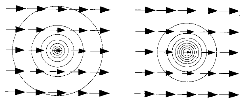
Figure 1: Distribution of postshock velocity vectors for a linear shock passing (from left to right) through a circular cloud, ignoring effects such as cloud compression or shock curvature. The size of each arrowhead is proportional to the postshock speed at that position. The density distributions are power laws with indices -1 (a) and -2 (b), and density contours are indicated by the circular lines. In this case the kinematic vorticity is due to the derivative of the postshock velocity along the shock line.

Our model consists of a planar shock of speed $v_{sh}$, propagating in the x-direction, incident on a spherically symmetric centrally condensed cloud whose density distribuition $\rho(r)$ joins smoothly with the ambient density $\rho_{a}$ at large r. For the purpose of the present paper we assume that the shock remains planar as it propagates through the cloud. The inclusion of the shock curvature (see Fleck 1991 for an ISM application) would increase the vorticity generation, and could be included iteratively using the formalism given here, but we postpone a treatment of curvature effects for simplicity. We also neglect the vorticity generated by Mach stem and related phenomena (see Klein et al. 1994; Chernin 1996 and references therein). For the case of a planar shock, the vorticity generation is then due to two distinct processes. The first process is purely kinematical, and arises because the postshock velocity depends on the preshock density, which varies radially through the cloud. A gradient in the normal component of the postshock velocity will then exist along the shock surface, which is the source of vorticity. We emphasize that this effect is purely kinematic in origin, and is not related to the baroclinic vector $\nabla p\times\nabla\rho$ or the dilatation term $\omega\nabla\cdot u$ in the vorticity equation, nor does it depend on the energy equation. As we show below, the process basically traces to the asymmetry between conservation of normal and tangential momentum components at a discontinuity. For the simple model considered here, the passage of the shock will also generate a gradient of the postshock velocity perpendicular to the shock surface (i.e. along the x-axis) which is identical to the vortical gradient, but rotated by $\pi/2$. In the uniform cloud density case this component would be identified with a compression and acceleration of the cloud.

The second process results from the amplification or decay of the kinematically-produced vorticity by the flow field further downstream in the postshock flow, due to the baroclinic and dilatation terms in the vorticity equation. Although we have included this second process of “dynamical vorticity production” in our full calculations (Kornreich & Scalo 2000, in preparation, hereafter KS00), it is mathematically much more complicated, since it involves the evaluation of the flow derivatives from the full hydrodynamic equations. Our results (KS00) show that the vorticity change due to this process is generally much smaller than the kinematic effect, except for Mach numbers very close to unity, so we omit it here in order to give a more concise presentation.

We are conceptualizing the model “cloud” as imbedded in some uniform “intercloud medium.” The same shocks that we claim can drive dynamical motions within the cloud will also affect the intercloud gas, perhaps sweeping it away from the cloud, or, if the intercloud medium is inhomogeneous (in which case it can be regarded as other “clouds”), generating vortical and compressible velocity fluctuations there. Whatever the nature of these intercloud flows, they will have large speeds because of the lower density. However the present paper is only concerned with the velocity fluctuations induced within the cloud, and we do not pursue the interesting questions surrounding the fate of the intercloud gas.

In addition, it is likely that for some combinations of parameters, the shock-cloud interaction will lead either to disruption of the cloud or gravitational instability by compression. It is unclear what the shock and cloud parameters should be to arrive at these end states, so it must be remembered that we are only treating the cases in which the shock-cloud interaction leads to internal motions that do not disrupt the cloud or cause it to collapse. A very thorough simulation study of the collapse/dispersal question has been presented by Vanhala & Cameron (1998). However they concentrated on relatively large shock velocities and assumed cloud density distributions that were much more sharp-edge (e.g. Gaussian) than considered here. The fraction of parameter space occupied by our results is uncertain although we argue below that cloud disruption should occur in a small fraction of cases.

2.2 Outline of the derivation

Our treatment of kinematic vorticity induced by shock-density fluctuation interactions parallels the studies of curved shock vorticity by Truesdall (1952, 1954) and Hayes (1957). For a discussion of the MHD curved shock problem, see Ram (1967) and Ram & Upadhyaya (1968) and references therein. It is convenient to express the relevant equations in a coordinate system whose unit vectors, $\hat{n}$ and $\hat{\tau}$, are normal and tangential to the local shock surface. This transformation is especially useful in generalizing our results to include shock curvature and the presence of preshock velocity fluctuations (KS00).

It is useful to review the necessary transformations and derivatives relating to the coordinate vectors. In what follows, subscripts ijklm refer to cartesian coordinates, and, unless otherwise specified, summation over repeated indices is implied. A comma before a subscript denotes partial differentiation, e.g. $v_{i,j}\equiv\partial v_{i}/\partial x_{j}$. The components of a vector $v_{i}$ in this coordinate system are simply the normal component $v_{n}\equiv v_{i}n_{i}$ and the tangential component $v_{r}\equiv v_{i}\tau_{i}$. The normal component may be separated out by the relation

$$v_{i}-v_{n}n_{i}=\epsilon_{ijk}\epsilon_{klm}n_{j}v_{l}n_{m}\ .$$ (1)

where $\epsilon_{ijk}$ is the usual alternating permutation symbol. Since the normal and tangent vectors are gradients of the coordinates,

$$\epsilon_{ijk}n_{k,j}=\epsilon_{ijk}\tau_{k,j}=0.$$ (2)

Also, since they have fixed lengths,

$$n_{i,i}=\tau_{i,i}=0.$$ (3)

The directional derivatives are

$$n_{i}\nabla_{i}=\frac{\partial}{\partial n},$$ (4)

and

$$\tau_{i}\nabla_{i}=\frac{\partial}{\partial\tau}.$$ (5)

Finally, the normal derivatives of the unit vectors vanish. The tangential derivatives of the vectors, which are generally propotional to the curvature by the Frenet relations, are also taken as zero, since we are ignoring shock curvature.

The derivation of the kinematic shock-generated vorticity proceeds in three stages. First, we derive the general expression for the vorticity in normal-tangent coordinates; it is proportional to the difference between the normal derivative of the tangential velocity component, $u_{\tau,n}$, and the tangential derivative of the normal velocity component $u_{n,\tau}$. We then derive the shock jump conditions for this difference. The jump condition for the tangential component of the momentum equation yields an expression for the jump in the tangential derivative of the pressure $[p_{,\tau}]$ proportional to $[u_{\tau,n}]$, where brackets refer to changes across the shock. Taking the tangential derivative of the normal momentum jump condition gives another expression for $[p,_{\tau}]$ which is in this case proportional to $[u_{n,\tau}]$. Equating the two expressions for $[p,_{\tau}]$ results, after some manipulation, in the desired quantity $[u_{\tau,n}]-[u_{n,\tau}]$, and hence the vorticity jump. We restrict the analysis to two dimensions, partly for simplicity, and partly because we were interested in comparisons with two-dimensional simulations, to be presented elsewhere. Three-dimensional calculations of vorticity production by curved shocks in a medium without density fluctuations have been given by Hayes (1957) and Ram and Upadhyaya (1968).

2.3 Vorticity in the normal-tangent coordinate system

The velocity in the normal-tangent coordinate system is $u_{i}=u_{n}n_{i}+u_{\tau}\tau_{i}$. Then the vorticity is

$$\omega_{i} = \epsilon_{ijk}\nabla_{j}u_{k}=\epsilon_{ijk}\nabla_{j}(u_{n}n_{k}+u_{\tau}\tau_{k})$$ (6)

$$= u_{n}\epsilon_{ijk}n_{k,j}-\epsilon_{ijk}n_{j}u_{n,k}+\epsilon_{ijk}\nabla_{j}(u_{\tau}\tau_{k})$$

$$= \epsilon_{ijk}\nabla_{j}(u_{\tau}\tau_{k})-\epsilon_{ijk}n_{j}u_{n,\tau}\tau_{k}.$$

The last term involves only the tangential gradient because the normal gradient must vanish when crossed with the normal vector parallel to it.

In order to express the first term on the rhs of eq. 6 in a useful form, we use the orthogonality of the unit vectors to obtain

$$0=\nabla_{i}(u_{\tau}\tau_{j}n_{j})=\epsilon_{ijk}n_{j}\epsilon_{klm}\nabla_{l}(u_{\tau}\tau_{m})+\epsilon_{ijk}u_{\tau}\tau_{j}\epsilon_{klm}n_{m,l}+u_{\tau}\tau_{j}\nabla_{j}n_{i}+n_{j}\nabla_{j}(u_{\tau}\tau_{i}).$$ (7)

The second term on the right-hand side is zero because it contains a curl of a unit vector. The third and fourth terms are directional derivatives. Taking the first term on the left-hand side, and using the fact that $n_{i,\tau}=0$ for zero curvature shock surface, we find

$$\epsilon_{ijk}\epsilon_{jlm}n_{k}\nabla_{l}(u_{\tau}\tau_{m})=u_{\tau}n_{i,\tau}+\nabla_{n}(u_{\tau}\tau_{i})=u_{\tau,n}\tau_{i}.$$ (8)

Since in two dimensions the vorticity does not have a normal component, equation (1) may be used to obtain

$$\epsilon_{ijk}\nabla_{j}(u_{\tau}\tau_{k})=\epsilon_{ijk}n_{j}\epsilon_{klm}n_{m}\epsilon_{lqr}\nabla_{q}(u_{\tau}\tau_{\tau})=\epsilon_{ijk}n_{j}(u_{\tau,n}-\kappa u_{\tau})\tau_{k}.$$ (9)

Substituting (9) into (6) gives

$$\omega_{i}=\epsilon_{ijk}n_{j}(u_{\tau,n}-u_{n,\tau})\tau_{k}.$$ (10)

2.4 The Fluid Equations in the normal-Tangent Coordinate System

The equations of hydrodynamics in cartesian coordinates are the continuity equation

$$\rho_{,t}+u_{i}\rho_{,i}+\rho u_{i,i}=0\ ,$$

the momentum equation,

$$\rho u_{i,t}+\rho u_{j}u_{i,j}=-p_{,i}$$

and the energy equation,

$$p_{,t}+u_{i}p_{,i}+\gamma pu_{i,i}=0,$$

where $\rho$ is the density, $u_{i}$ is the ith component of the velocity in a cartesian coordinate system with $i$ ranging from 1 to 3, $p$ is the pressure, and $\gamma$ is the usual ratio of specific heats.

Expressed in normal-tangent coordinates, the continuity equation becomes

$$0 = \rho_{,t}+\nabla_{i}(\rho(u_{n}n_{i}+u_{\tau}\tau_{i}))$$ (11)

$$= \rho_{,t}+u_{n}n_{i}\nabla_{i}\rho+u_{\tau}\tau_{i}\nabla_{i}\rho+\rho(\nabla_{i}(u_{n}n_{i})+\nabla_{i}(u_{\tau}\tau_{i}))$$

$$= \rho_{,t}+u_{n}\rho_{,n}+u_{\tau}\rho_{,\tau}\rho u_{n,n}\rho u_{\tau,\tau},$$

where the vanishing of the divergence of the unit vectors was employed.

The momentum equation becomes

$$-\frac{1}{\rho}p_{,i}=u_{n,t}n_{i}+u_{r,t}\tau_{i}+(u_{n}n_{j}+u_{\tau}\tau_{j})\nabla_{j}(u_{n}n_{i}+u_{\tau}\tau_{i}).$$ (12)

The normal derivatives are

$$u_{n}n_{j}\nabla_{j}(u_{n}n_{i}+u_{\tau}\tau_{i})=u_{n}u_{n,n}n_{i}+u_{n}u_{\tau,n}\tau_{i}.$$ (13)

The tangential derivatives are

$$u_{\tau}\tau_{j}\nabla_{j}(u_{n}n_{i}+u_{\tau}\tau_{i})=u_{\tau}u_{n,\tau}n_{i}+u_{\tau}u_{\tau,\tau}\tau_{i}.$$ (14)

The above equations can be combined to give the normal

$$\rho(u_{n,t}+u_{n}u_{n,n}+u_{\tau}u_{n,\tau})=-p_{,n}$$ (15)

and tangential

$$\rho(u_{\tau,t}+u_{n}u_{\tau,n}+u_{\tau}u_{\tau,\tau})=-p_{,\tau}$$ (16)

components of the momentum equation.

The energy equation becomes

$$0 = p_{,t}+(u_{n}n_{i}+u_{\tau}\tau_{i})\nabla_{i}p+\gamma p\nabla_{i}(u_{n}n_{i}+u_{\tau}\tau_{i})$$ (17)

$$= p_{,t}+u_{n}p_{,n}+u_{\tau}p_{,\tau}+\gamma p(u_{n,n}+u_{\tau,\tau}).$$

2.5 Oblique Shock Jump Conditions

Let the quantities in front of the shock be labeled with subscript 0. These are the preshock density $\rho_{0}$, pressure $p_{o}$, and velocity $u_{o}$. The respective postshock quantities ($\rho,\ p,\ u_{i}$) will have subscript 1. For the shock jump conditions, we introduce the notation $[a]\equiv a_{1}-a_{0}$. Then the shock jump conditions are mass conservation

$$[\rho u_{n}]=0,$$ (18)

normal momentum conservation

$$[p+\rho u^{2}_{n}]=0,$$ (19)

tangential momentum conservation

$$[u_{\tau}]=0\ ,$$ (20)

and energy conservation

$$\left[\frac{1}{2}u^{2}_{n}+\frac{\gamma}{\gamma-1}\frac{p}{\rho}\right]=0.$$ (21)

By equation (18)

$$[u_{n}]=(\rho_{0}u_{0n}/\rho)-u_{0n}=u_{0n}(\rho_{0}-\rho_{1})/\rho_{1}.$$ (22)

For determining the change in vorticity it is convenient to introduce the relative density jump,

$$\Delta\equiv(\rho_{1}-\rho_{0})/\rho_{0}.$$ (23)

Then $\rho=(1+\Delta)\rho_{0}$ and $\rho_{0}-\rho_{1}=-\Delta\rho_{0}$, so

$$[\rho]=\Delta\rho_{0}$$ (24)

and

$$[u_{n}]=-u_{0n}\Delta/(1+\Delta).$$ (25)

Using (18) and (19), the pressure jump is

$$[p]=-[\rho u^{2}_{n}]=-\rho_{0}u_{0n}[u_{n}].$$ (26)

Let $c_{s}\equiv\sqrt{\gamma p_{0}/\rho_{0}}$ be the sound speed. Then the Mach number is $M\equiv u/c_{s}$. However, for an oblique shock, it is convenient to introduce the quantity $M_{n}\equiv u_{n}/c_{s}$. Then combining equations (18–21) gives the solutions

$$\rho_{1}=\frac{(\gamma+1)M^{2}_{n}}{(\gamma-1)M^{2}_{n}+2}\rho_{0}$$ (27)

and

$$p_{1}=\frac{1+\gamma(2M^{2}_{n}-1)}{\gamma+1}p_{0}$$ (28)

2.6 Vorticity Jump Condition

The jump condition for the tangential component of the momentum equation (16) is found by substituting eqs. 18 and 20, and using the fact that $u_{\tau,\tau}=0$ for non-curved shocks. The result is

$$-[p_{,\tau}]=\rho_{0}u_{0n}[u_{\tau,n}]+[\rho]u_{0\tau}u_{0\tau,\tau}=\rho_{0}u_{0n}[u_{\tau,n}].$$ (29)

Next, the tangential derivative of the normal momentum jump condition (19) gives, using eq. (18)

$$-[p_{,\tau}]=\delta_{\tau}u_{0n}[u_{n}]+\rho_{0}u_{0n,\tau}[u_{n}]+\rho_{0}u_{0n}[u_{n,\tau}].$$ (30)

Finally, we need an expression for $u_{0n,\tau}$, which we next derive for isobaric preshock density fluctuations, under the assumption that the postshock pressure is constant along the shock. This assumption depends on, among other things, considerations of the effect of a reflected shock on the postshock environment. An estimate for the magnitude of this effect on the constant postshock pressure assumption is attempted in the Appendix.

We now turn to the derivation of $u_{0n,\tau}$, which occurs in eq. (30). Because the shock jump conditions involve the quantities where the shock is at rest, we consider infinitesimal regions of the shock line such that a transformation may be made to a coordinate system such that adjacent regions along the shock line are also at rest. Since the preshock velocity is assumed to be zero, at any point in this frame $u_{0\tau}=0$, and the normal component $u_{0n}=-v_{sh}=-Mc_{0}$. In this case

$$u_{0n,\tau} = -\frac{\partial v_{sh}}{\partial\tau}$$ (31)

$$= -\frac{\partial}{\partial\tau}\left(M\sqrt{\gamma p_{0}/\rho_{0}}\right)$$

$$= -M_{,\tau}\sqrt{\frac{\gamma p_{0}}{\rho_{0}}}-\frac{Mp_{0,\tau}}{2}\sqrt{\frac{\gamma}{p_{0}\rho_{0}}}-M\sqrt{\gamma p_{0}}\left(-\frac{1}{2\rho^{3/2}_{0}}\delta_{\tau}\right)$$

$$= -\frac{M_{,\tau}v_{sh}}{M}-\frac{v_{sh}p_{0,\tau}}{2p_{0}}+\frac{v_{sh}\delta_{\tau}}{2\rho_{0}}$$

$$= \frac{M_{,\tau}u_{0n}}{M}+\frac{u_{0n}p_{0,\tau}}{2p_{0}}-\frac{u_{0n}\delta_{\tau}}{2\rho_{0}}$$

In the above expressions we denote the tangential derivative of the preshock density by

$$\delta_{\tau}\equiv\partial\rho_{0}/\partial\tau$$ (32)

In this frame, because the tangential gradient of the normal velocity does not vanish, it may appear that there is some pre-existing vorticity in the preschock region. However, this is not the case. Because the different parts of the shock line are not traveling at uniform speed, a transformation to a frame in which the shock line is at rest is not a Galilean transformation. This is why infinitesimal regions must be considered.

In the isobaric case, the second term in equation (31) vanishes by definition. Also, since the pressure in front of the shock is constant (by the isobaric assumption) and the pressure behind the shock is constant (by the main assumption of this section), the pressure jump is constant along the shock. By the equation for the pressure jump across the shock (28), the only way that can occur is if the Mach number $M=$ constant. (It is important to notice that this is the only point in the derivation where the energy equation is used.) Therefore, the first term also vanishes.

Then equation (31) reduces to

$$u_{0n,\tau}=-\frac{u_{0n}\delta_{\tau}}{2\rho_{0}}$$ (33)

Substituting eq. (33) for $u_{0n,\tau}$ in eq. (30) gives

$$-[p_{,\tau}]=\delta_{\tau}u_{0n}[u_{n}]+\rho_{0}u_{0n}[u_{n,\tau}]$$ (34)

where $\delta_{\tau}=\partial\rho_{0}/\partial\tau$. Equating the two expressions (34) and (29) and using the jump condition $[u_{n}]=-u_{0n}\Delta/(1+\Delta$), where $\Delta=(\rho_{1}-\rho_{0})/\rho_{0}$ is the fractional density jump, gives

$$[u_{\tau,n}]-[u_{n,\tau}]=\frac{\delta_{\tau}}{\rho_{0}}\frac{u_{0n}\Delta}{(1+\Delta)}$$ (35)

Substitution into eq. (10) for the tangential vorticity component, assuming no vorticity in the preshock cloud, and using $u_{0n}=-v_{sh}$ (in the shock frame) finally gives the generated kinematic vorticity just behind the shock at any position ($r,\theta$) in the cloud as

$$\omega(r,\theta)=v_{sh}(r)\delta_{\tau}(r,\theta)\Delta/\rho_{0}(r)(1+\Delta).$$ (36)

Eq. (36) is the main result of this section. For an isobaric preshock density distribution this expression gives the kinematically generated vorticity as a function of position due to the passage of the shock. It should be noted that we have neglected the compression of the cloud by the shock passage, which is why the radial coordinates on the lhs and rhs of eq. (36) refer to the same position.

3 SHOCK INTERACTION WITH A RADIAL DENSITY GRADIENT

3.1 Spatial dependence of kinematic shock-generated vorticity

We evaluate the shock-induced vorticity as a function of position in the cloud for the following density distribution:

$$\rho_{o}(r)=\rho_{a}+\frac{\rho_{c}-\rho_{a}}{1+(r/R_{o})^{n}}=\rho_{a}\left(\frac{\xi+\chi-1}{\xi}\right)$$ (37)

where $\xi(r)\equiv 1+(r/R_{o})^{n}$, $R_{o}$ is a characteristic radius, and the density contrast is $\chi\equiv\rho_{c}/\rho_{a}$. We have also considered an exponential density distribution, but the algebra is sufficiently complicated, and the results so similar, that we only indicate the differences when appropriate.

For the power law density distribution the tangential density derivative is (neglecting the curvature)

$$\delta_{\tau}(r,\theta)=\frac{\partial\rho_{a}}{\partial y}=-\rho_{a}(\chi-1)nr^{n-1}\ {\rm sin}\theta/R_{o}^{n}\xi^{2}$$ (38)

The shock speed $v_{sh}$ in the cloud is a function of radius, and can be expressed in terms of the incident shock speed $v_{\infty}\left(={\mit M}\sqrt{\frac{\gamma p_{o}}{\rho_{a}}}\ \right)$ by

$$v_{sh}(r)=v_{\infty}[(\xi/(\xi+\chi-1)]^{1/2}\ .$$ (39)

Also, notice that for the isobaric clouds considered here, the pressure difference across the shock interface is constant along the shock surface, so the Mach number and $\Delta$ are constant. Combining these factors in eq. (36) gives

$$\omega(r,\theta)=-\frac{nv_{\infty}\Delta(\chi-1)}{2(1+\Delta)R_{o}^{n}}\ \frac{r^{n-1}\ {\rm sin}\theta}{(\xi+\chi-1)^{3/2}\xi^{1/2}}$$ (40)

Because of the sin$\theta$ factor, the vorticity will be concentrated in regions above and below (along the y-axis) of the center of the cloud. The dependence on $\xi$ tends to make these regions flattened along the y-axis. The ratio of specific heats $\gamma$ and the Mach number of the incident shock $M=v_{sh}/c_{s}$ (= constant) enter through the fractional density jump given by $1+\Delta=(\gamma+1)M^{2}/[(\gamma-1)M^{2}+2]$, which for a strong shock is independent of $M$ and equals 4 for $\gamma=5/3$.

Figure 2 shows a grey-scale representation of the induced vorticity given by eq. (40) (or its equivalent for the exponential density distribution) for four forms of the density distribution, with central density enhancement $\chi=10$. Figure 3 shows the angle-averaged radial distribution of vorticity (in units of the shock velocity divided by $R_{o}$) for the same four density distribution, each for four values of $\chi$. It can be seen that increasing the density contrast $\chi$ causes the position of peak induced vorticity to shift further away from the center of the cloud relative to the scale radius $R_{o}$. The important point is that, unless the density gradient is very steep or the density contrast very large, much of the vorticity is generated well inside the cloud.

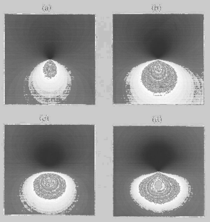
Figure 2: Greyscale map of the induced kinematic vorticity within a model cloud for power law density distributions with $n=1$ (a), $n=3/2$ (b), $n=2$ (c), and for an exponential density distribution (d). The density contrast is $\chi=10$ and each map extends to 5 scale radii.

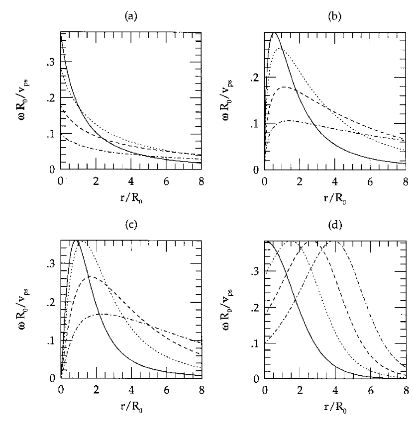
Figure 3: Angle-averaged radial dependence of shock-induced kinematic vorticity, in units of postshock speed divided by scale radius, for the four density distributions (three power laws and an exponential) used in Fig. 2. The solid lines correspond to density contrast $\chi=3$, dotted lines to $\chi=10$, dashed lines to $\chi=30$, and dashed-dotted lines to $\chi=100$.

3.2 rms kinematic vorticity

In order to characterize the magnitude of the kinematically-generated vorticity due to the shock passage, we calculate the rms vorticity in a region of size $R$ and mass $m$:

$$\omega_{rms}\equiv\left[\frac{1}{m}\int\rho\omega^{2}dA\right]^{1/2}=\left(\frac{1}{m}\int^{R}_{0}\int^{2\pi}_{0}\ \rho(r)\omega^{2}(r,\theta)rdrd\theta\right)^{1/2}$$ (41)

Letting $z\equiv R/R_{o}$, we find

$$\int\rho\omega^{2}dA=\frac{\pi\rho_{a}\Delta^{2}v^{2}_{\infty}n}{4(\Delta+1)^{2}}\times\left[\frac{(\chi+1)\ell n\left(\frac{(1+z^{n})\chi}{\chi+z^{n}}\right)}{\chi-1}+\frac{1}{1+z^{n}}+\frac{\chi}{\chi+z^{n}}-2\right]$$ (42)

The mass m contained in a region of radius $R$ is given by $m=2\pi\int^{R}_{0}\rho(r)rdr$. For the density distribution given by eq. (37), the integral can be obtained in closed form for only selected values of the exponent $n$. For the cases $n=1$, 3/2, and 2 we find

$$m=\rho_{a}\pi R_{o}^{2}[z^{2}+b(\chi-1)]$$ (43)

where $b=2[z-\ell n(1+z)]$ for $n=1$ and $b=\ell n(1+z^{2})$ for $n=2$. For $\chi\ll z^{2}$, the first term dominates and $m$ is independent of the density contrast $\chi$, while in the limit of large $\chi,\ m\propto\chi$, as expected. For $n=3/2$ and for an exponential density distribution the expression for $b$ is more complicated, but m has the same limits, and we assume that the small and large $\chi$ results are general.

In the limit $\chi\rightarrow 1(\chi\ll z^{2})$, the integral (42) can be shown to be proportional to $\chi-1$ and m (eq. 43) is independent of $\chi$, so $w_{rms}\propto(\chi-1)^{1/2}$. In the large $\chi$ limit, the integral (42) is

$$\int\rho\omega^{2}dA=\frac{\pi\rho_{a}\Delta^{2}v^{2}_{\infty}n}{4(\Delta+1)^{2}}\times\left[\ell n(1+z^{n})+\frac{1}{1+z^{n}}-1\right]^{1/2}$$ (44)

independent of $\chi$. Since the mass is proportional to $\chi$ for $\chi\gg z^{2}$, $\omega_{rms}\propto\chi^{-1/2}$ in the large $\chi$ limit.

For an exponential density distribution the algebra is more complicated, but the same results for the $\chi$-dependence are found in the small- and large-$\chi$ limits.

The result that $\omega_{rms}$ scales with density contrast as $\chi^{-1/2}$ in the limit of large density contrast is different than found by Klein et al. (1994) for a sharp-boundaried cloud, who found that the average vorticity is independent of $\chi$ in the large $\chi$ limit. The reason for this difference is that for a sharp-boundaried cloud the vorticity is confined to a small boundary layer, and so depends on the difference between the postshock speeds inside the cloud and in the ambient medium. This difference, which is proportional to ($1-\chi^{-1/2}$), is constant and equal to 1 for large $\chi$. For clouds with a continuous density gradient the vorticity is located inside the cloud and thus just depends on the postshock speed in the cloud. As discussed above, the average postshock speed inside the cloud is proportional to $\chi^{-1/2}$.

It is useful to re-express the above results in terms of the quantity $\beta_{kin}=w_{rms}/(v_{\infty}/R)$, which may be considered as the ratio of the characterstic vortical velocity $v_{vor}\equiv w_{rms}R$ to the shock speed in the ambient medium $v_{\infty}$. In the limit of large $\chi$ and $z>1$ we find

$$\beta_{kin}=\frac{\Delta zn^{1/2}}{2(\Delta+1)\chi^{1/2}}\left(\frac{\ell n(1+z^{n})}{f(z)}\right)^{1/2}$$ (45)

where $f(z)=2z$, 4z^1/2, and $\ell n(1+z^{2})$ for $n=1$, 3/2, and 2, respectively. Assuming $z\sim 1$,

$$v_{vor}/v_{\infty}\approx\frac{\Delta n^{1/2}}{2(\Delta+1)}\chi^{-1/2}$$ (46)

For the exponential density distribution, the coefficient is $\Delta/[2\sqrt{2}(\Delta+1)]$. In the limit of large Mach number, $\Delta/(\Delta+1)=3/4$ for $\gamma=5/3$, or $\sim 1$ for $\gamma=1$. So for large $\chi$ and $M$, a fraction $3\sqrt{n}\chi^{-1/2}/8\ (3\chi^{-1/2}/8\sqrt{2}$ for an exponential distribution) of the ambient shock speed may be transmitted into a cloud as a vortical mode.

The amplitude and dependence on Mach number and density contrast predicted by eq. 46 have been checked by comparison with lattice gas hydrodynamical simulations of shock-cloud interactions in two dimensions (Kornreich & Scalo 2000). Because of the nature of the lattice-gas method, only simulations with Mach numbers up to about 3 were possible. However, within this constraint, the simulations (which include the flattening of the cloud and the shock curvature) show good agreement with eq. 46. In addition, the simulations verify that most of the vorticity is generated as two oppositely-signed vortices within the cloud (rather than a vorticity sheet at the surface), and that there is little tendency for cometary morphology after shock passage, or shredding from the outer layers of the cloud, as has been found in previous simulations of sharp-edged clouds (see sec. 3.6. below), at least for the modest Mach numbers accessible to the simulations. The simulations also verify that the dynamical vorticity generation (as opposed to the kinematic vorticity generation studied here) is negligible except at Mach numbers close to unity.

3.3 Density scaling

Figure 4 shows $\beta_{kin}$, calculated using eqs. 43–45 (or, for eqs. 42 and 44, from the corresponding equations for the exponential case), as a function of $\chi$, for four different density distributions and four Mach numbers. The adiabatic index was taken to be $\gamma=5/3$. Changing the adiabatic index to $\gamma=1$ only increases $\beta_{kin}$ slightly, since then, for example, $\Delta/(\Delta+1)\approx 1$ instead of 3/4 at large Mach numbers. The radial limit of integration was taken as $R/R_{o}=2$. The shape of the curves does not depend on the adopted density distribution; only the maximum value of $\beta_{kin}$ and the value of $\chi$ for which it occurs depend on the density distribution, and only weakly. The plots illustrate the limiting forms given earlier. However notice that the $\chi^{-1/2}$ dependence is only valid for density contrasts greater than about 6–10. At small density contrast the curves increase with $\chi$, roughly in agreement with the ($\chi-1)^{1/2}$ dependence (which is a steep function for $\chi\approx 1$) predicted above.

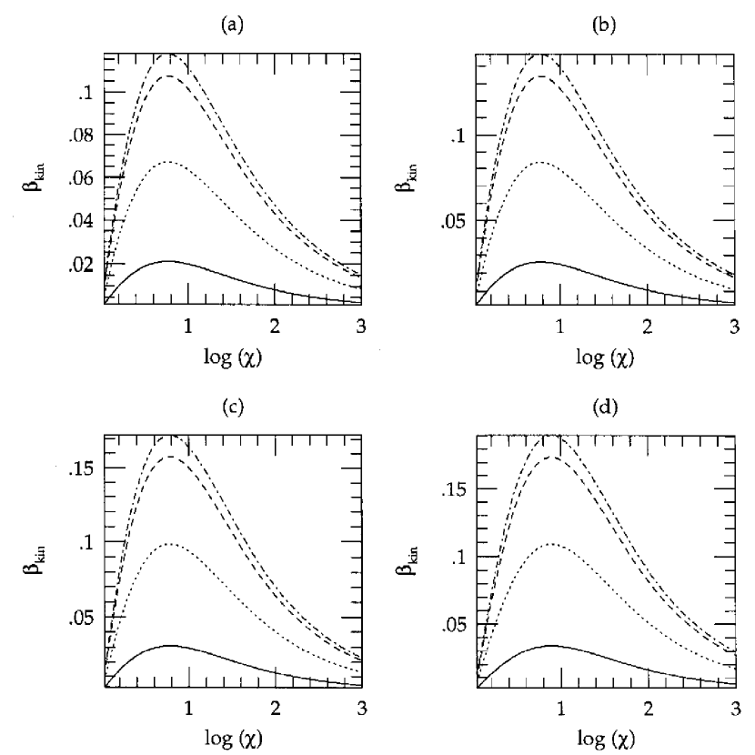
Figure 4: Ratio of the characteristic induced kinematic vortical speed $\omega_{rms}$R to the shock speed in the ambient medium as a function of the logarithm of the density contrast $\chi$ for $\gamma=5/3$ and a radial integration limit $R/R_{o}=2$. The four panels correspond to power law density distributions with indices 1 (a), 3/2 (b), 2 (c) and an exponential distribution (d). In each panel the curves correspond to Mach numbers of 1.1 (solid), 1.5 (dotted), 3 (dashed), and 6 (dashed-dotted).

The scaling predicted by Chernin and collaborators (Chernin 1996 and references therein), which is based on a scattering approach that assumes small $\chi$ and large Mach number, also increases with $\chi$. They give the dependence of the spatially maximum value of $\beta$ as proportional to $\chi$, while we derive the rms value of $\beta$, so it isn’t clear whether there is a discrepancy. In any case, we have not assumed either small density contrasts or large Mach numbers in the above derivation, and our small-$\chi$ case is just a limit of the general case, while Chernin et al. assume both limits at the outset. Given that the $\chi$-dependence changes its functional form at larger density contrast, it is inappropriate to apply the small-$\chi$ case to cloud complexes, GMCs, etc. as do Chernin and Efremov (1995). However it is still important to note that the spatial distribution of vorticity found in their quasi-hydrodynamical simulations, which still use the assumptions of small density contrast and large Mach number to calculate velocity perturbations behind the shock, is similar to that found here, namely two counter-rotating vortices. Chernin and Efremov also illustrate interesting cases of a shock passing obliquely through an elongated two-dimensional cloud, and a three-dimensional calculation.

3.4 Validity of the frozen vorticity assumption

The above derivation assumes that the induced vorticity does not change during the shock passage through the cloud. The viscous decay time is of order $\tau_{vis}\sim\ell^{2}/\lambda v_{th}$ where $\ell$ is the scale on which the vorticity is generated, $\lambda$ is the mean free path, and $v_{th}$ is the thermal speed. Taking $\lambda=1/n\sigma$, where $n$ is the number density and $\sigma$ is the particle cross section, and assuming $\sigma\sim 10^{-15}cm^{2}$ and $n\sim 10^{3}R_{pc}^{-1}cm^{-3}$ for illustration, we find

$$\tau_{vis}\sim 3\times 10^{6}\ell^{2}/Rv_{th},$$ (47)

which is much larger than the timescale for shock passage, $\tau_{sh}\equiv R/v_{sh}$ for any reasonable value of $\ell$. However the induced vorticity will also change due to conversion into other fluid modes (dilatation, MHD modes; see below). The timescale for these changes is expected to be of order $\tau_{vor}\sim R/v_{vor}$. Then $\tau_{vor}/\tau_{sh}=2[(\Delta+1)/\Delta]\ell/R$ which, for large Mach number, is (8/3)$\ell$/R for $\gamma=5/3$ and 2 $\ell$/R for $\gamma=1$. So while the vorticity is not strictly “frozen,” the vorticity should not change appreciably during shock passage. The frozen vorticity assumption becomes better for weaker shocks.

3.5 Compressional and bulk components

For the conditions studied here, the local induced motions within the cloud should initially be composed equally of compressional and vortical modes. The conditions that provide this equivalence are the radially symmetric density gradients and the nonoblique shock. Since the density gradient is radially symmetric, the density gradients parallel and perpendicular to the shock propagation direction are equal. Taking into account the assumption about the constant pressure behind (and in front of) the shock, by momentum conservation across the shock, the postshock velocity gradients are determined by the preshock density gradients, and therefore should also be symmetric (ignoring such distortions as cloud flattening). Therefore, since the vorticity may be thought of as the gradient in the velocity perpendicular to the direction of the shock propagation, and the dilatation is due to gradients in the velocity parallel to the direction of the shock propagation, the vorticity and the dilatation should be comparable. The nonoblique condition means that the cloud had no (initial) tangential velocity relative to the shock. Thus, the postshock velocity is dominated by motions in the direction of the shock (i.e. the component of the velocity perpendicular to the shock propagation, which would be conserved across the shock, is small). It follows from these two conditions that since the only source of the velocity behind the shock is the momentum imparted from the shock, and the gradients of the postshock velocity parallel and perpendicular to the shock propagation are equivalent, then the vortical and compressional components of the velocity must be (approximately) equal. In a statistical sense, the same conclusion may be drawn for any inhomogeneous density medium that does not have a preferential gradient; i.e. the average compressional and vortical velocities should be comparable. An example of the violation of the nonpreferential density gradient would be if, say, all the clouds were prolate with their long axes in the direction of the shock. The reason that this effect (i.e. the equivalence of the vortical and compressional velocities) would be violated for an oblique shock is the differences in the way the curl and the divergence are taken and, in particular, the manner in which the gradients of the tangential component of the velocity are affected by the shock. Because of the curvature of the shock near the center of the cloud, oblique shock effects will also occur even in the case of symmetric preshock gradient, and therefore any distortions in the regions where the shock is significantly curved will not be transitory. Still, to first order it is expected that the compressional and vortical velocities, at least initially, should be comparable.

Besides the internal vortical and compressional modes excited by the shock, the shock also accelerates the whole cloud. The bulk cloud speed is the average postshock speed $v_{ps}$ in the cloud:

$$v_{cl}=\int\rho v_{ps}(r)/m$$ (48)

The postshock speed is $v_{ps}=\frac{\Delta}{\Delta+1}v_{sh}(r)$, where $v_{sh}(r)$ is given by eq. (41). Taking $\Delta/(\Delta+1)$ out of the integral because of the constant Mach number assumption, we find, for large $\chi$,

$$v_{cl}=\frac{\Delta}{\Delta+1}\chi^{-1/2}v_{\infty}\ .$$ (49)

This result is actually the same as that for a cloud with a sharp boundary (McKee & Cowie 1975, Miesch & Zweibel 1994). The reason for the equivalence is that in the limit of large $\chi$, the mass in the continuous case is more concentrated in the center of the cloud, and thus the mass weighted bulk motion approaches the velocity at the center of the cloud. Using the induced vortical velocity from eq. (48), taking $n\approx 1$, this gives $v_{cl}\approx 2v_{vor}$. By the argument of the previous paragraphs the vortical velocity is about equal to the compressional velocity $v_{comp}$, so $v_{cl}\approx v_{vor}+v_{com}$, and there is approximate equipartition between the bulk cloud speed and the total induced internal motions. Notice that the definition of the “large $\chi$ limit” ($\chi\gg(R/R_{o})^{n}$) depends on the limit of integration and $n$, since for larger R the now fast-moving material is averaged with the cloud speed, but the gradient in the velocity is smaller; also, in the central regions the shock curvature will be significant. However, since the location of maximum vorticity is away from the center, this result should be valid to order of magnitude.

3.6 Comparison of induced velocity amplitudes with observations

Both the internal and bulk components of the shock-induced velocity scale with cloud density as $\rho^{-1/2}$. Although we do not wish to place too much emphasis on this result until the statistical correlations for an ensemble of shock-cloud interactions is calculated, it may be significant that the “standard” empirical scaling relations give this same linewidth-density scaling if size is eliminated, and it may be, as suggested by Xie (1997) for a very different model, that it is the linewidth-density scaling that is most physically fundamental. If $\rho\propto R^{-1}$, as is often claimed, the induced motions, whether for the internal motion or for an ensemble of clouds, would satisfy a linewidth-size relation $\Delta v\propto R^{1/2}$. We are unable to justify such a density-size relation, since we cannot derive the characteristic sizes of the induced velocity and density fluctuations analytically. However the $\Delta v\propto R^{1/2}$ relation in the sense of a scaling of the velocity structure function at least will automatically be satisfied by an uncorrelated field of discontinuities (Saffman 1971), although modifications will certainly appear in more realistic situations. In this case the shock pump could in principle account for both observed (uncertain) scaling relations, without requiring self-gravity, magnetic fields, or internal protostars.

More importantly for the present work, the shock-induced velocities are consistent with the amplitudes of the observed linewidths. If we identify the shock with supernova remnants or superbubbles, the most frequent shock speed by far will be the terminal speed (because the distribution of shell speeds is a strongly decreasing function of speeds, see sec. 4 below), which is usually taken to be $\sim 10km\ s^{-1}$. Assuming $\rho\sim R^{-1}$ for illustration, on the large end of the spectrum of GMC sizes, 100 pc, we find $\Delta v\sim\frac{\Delta}{2(\Delta+1)}R^{1/2}\sim(3-8)R^{1/2}_{100pc}\ km\ s^{-1}$. If smaller clouds are nested within these larger structures, then the transmitted shock from the shock passage through the larger cloud is decreased by a factor of $\chi^{-1/2}$, giving the correct amplitude for the smaller scales. Of course this argument is too crude, since shocks will be generated within clouds of various densities. A treatment of the relation between the statistical properties of the density and velocity fluctuations is postponed to future work.

There is an important difference between the morphology of shocked clouds predicted by the present model and that predicted by previous simulations of shocks incident on clouds with sharp boundaries. In the latter case the vorticity is generated in a sheet at the model cloud surface, and this material is swept behind the cloud by the shock, resulting in comet-shaped clouds (or filaments with “heads”). Such structures are found even in simulations of low-velocity shock-cloud interactions (Horvath & Toth 1995). However the point of the present work is that, when the cloud possesses a continuous density gradient, most of the vorticity is generated within the cloud, not at its boundary, and thus there is much less tendency for the shock to “shear off” the edge of the cloud. Two-dimensional lattice gas simulations of shock-cloud interactions up to Mach numbers of 3 (KS00) confirm this picture: the simulated clouds flatten during the shock passage, but most of the vorticity generation is internal and little of the exterior portions of the cloud are “shredded.” At larger Mach numbers the shredding may be more significant because of the increased flattening (or instabilities, see Schiano et al. 1995), but in general we do not predict the degree of cometary, or head-tail, structure predicted by previous studies of sharp-edged clouds. Therefore, although some cometary structures are observed in the ISM, the fact that most clouds do not exhibit such structure may be interpreted as support for our model.

3.7 Fate of the induced vorticity

The kinematic vorticity generated by a shock passing through a density inomogeneity is unlikely to remain in the vortical mode for long. In sec. 3.4. we showed that the viscous decay is negligible. The vorticity could be amplified in the postshock flow by the baroclinic vector due to the generally non-parallel pressure and density gradients in the postshock flow, but an analysis of this effect (KS00) indicates that the vorticity amplificaton will be negligible except at Mach numbers close to unity. In three dimensions, the vorticity can amplify or suppress itself through the vorticity stretching term in the momentum equation, but there is good reason to think that the dominant process will be the conversion of vorticity into compressible modes.

One way to see this is to examine the evolution equations for the vorticity $\omega=(\nabla\times u$) and the dilatation $\theta\equiv\nabla\cdot u$. Taking the curl of the momentum equation, the evolution equation for a component $\omega_{i}$ of the vorticity can be shown to be

$$\frac{d\omega_{i}}{dt}=\omega_{j}\sigma_{ij}-\frac{2}{3}\theta\omega_{i}-\frac{\epsilon_{ijk}p_{ij}\rho_{jk}}{\rho^{2}}$$ (50)

where $\sigma_{ij}$ is the symmetric shear tensor given in terms of the velocity gradient tensor $\psi_{ij}\equiv u_{i,j}$ by

$$\sigma_{ij}\equiv\frac{1}{2}[\Psi_{ij}+\Psi_{ji}]-\delta_{(ij)}\Psi_{ij}/3\ ,$$ (51)

where the parentheses on the subscripts of the Kronecker delta indicate that there is no summation. The first two terms on the right-hand side of eq. (50) are equivalent to the vorticity stretching term $\omega\cdot\nabla u$, but we have decomposed the velocity gradient tensor to make explicit the interaction between vorticity and dilatation. See Peebles (1993, sec. 22) for a similar derivation in a cosmological context. In terms of the positive quantity $\omega\equiv(\omega_{i}\omega_{i})^{1/2}$ the vorticity equation becomes

$$\frac{dw}{dt}=\frac{1}{\omega}\omega_{i}\omega_{j}\sigma_{ij}-\frac{2}{3}\theta\omega-\frac{\omega_{i}\epsilon_{ijk}p_{,j}\rho_{,k}}{\omega\rho^{2}}\ .$$ (52)

The divergence of the momentum equation gives

$$\frac{d\theta}{dt}=\frac{1}{2}\omega^{2}-\sigma^{2}_{ij}-\frac{1}{3}\theta^{2}-\frac{1}{\rho}\nabla^{2}p+\frac{\rho_{,i}p_{,i}}{\rho^{2}}\ .$$ (53)

Ignoring all terms besides the explicit vorticity-dilatation interactions, it can be seen that there is an asymmetry between the two equations. The magnitude of the vorticity can only decrease due to the vorticity-dilatation interaction, but this vorticity always increases the dilatation. Another way to see this is to examine the evolution equation for the ratio of vorticity magnitude to dilatation. Again neglecting all terms except those explicitly involving the vorticity and dilatation, the result is

$$\frac{d(\omega/\theta)}{dt}=-\frac{\omega}{3}-\frac{\omega^{3}}{2\theta^{2}}$$ (54)

This asymmetry (in a somewhat different form) was pointed out independently by Vazquez-Semadeni, Passot, & Pouquet (1996), who also present evidence from simulations that, in highly compressible flows, vortex stretching acts primarily to drain the vorticity. Additional support for the dominance of transfer from vortical to compressible modes comes from the eddy-damped quasinormal Markovian closure analysis of weakly compressible turbulence by Bataille & Zhou (1999). The ability of a purely incompressible (vortical) velocity field to generate density fluctuations is also shown in the 2-dimensional simulations of Chantry, Grappin, & Leorat (1993) for a simple initial velocity field.

The upshot is that we expect the shock-generated vorticity to be converted to compressible modes, and the associated density inhomogeneities (since $d\ell n\rho/dt=-\theta$). It is important to realize that this mechanism provides a source of large-amplitude density fluctuations that do not owe their origin to any sort of instability, gravitational or otherwise. Since the induced vortical velocities are generally supersonic for the interstellar conditions considered here, we expect the induced vorticity to result in a system of internal shock waves, which themselves will generate their own kinematic vorticity and dilatation on smaller scales. Thus shock-generated kinematic vorticity provides a mechanism for top-down cascade of kinetic energy and creation of a nested system of density fluctuations. We suggest that this process could be at least part of the physics behind the observed fractal-like structure of the cool interstellar medium, an empirical property that has many potentially important implications (Elmegreen & Falgarone 1996, Elmegreen 1997a,b).

There is ample evidence that complex density structure exists in regions in which self-gravity is unimportant and there are no stellar power sources. A good example is the densely sampled map of the “Polaris Flare” cloud by Heithausen & Thaddeus (1990). The study of the cloud MBM 12 (size $\sim$2 pc) by Pound et al. (1992) reveals numerous “clumps” with supersonic linewidths and sizes down to the resolution limit of $\sim$0.03 pc. Similar results have been obtained for the cloud MBM 7 by Minh et al. (1996), who suggest that the large turbulent linewidths and density structure in this and other non-self-gravitating molecular clouds are due to the passage of a shock. High-resolution CCS maps of core D in TMC 1 in Taurus by Langer et al. (1995) show evidence for very small condensations with sizes of order 0.01 pc (and narrow lines), and point out that these condensations are unlikely to be the result of gravitational instability. These observations are consistent with the picture outlined in the present work, which provides a specific mechanism for the production of internal velocity and density structure on a large range of scales without the necessity of any sort of instability.

The timescale for conversion of the induced vortical motions into compressible modes should be on the order of the cloud size divided by the induced vortical velocity for the model shock-cloud system considered here. However the present model is highly idealized, and in a more realistic situation the shock will be corrugated and the cloud will contain pre-existing density fluctuations, so the appropriate size scale and timescale should be smaller.

Schiano, Christiansen, & Knerr (1995) performed two-dimensional simulations that are relevant to the present work. Although their study was concerned with high-speed winds interacting with clouds that are initially ram-pressure confined, the results demonstrate the ability of shock-cloud interactions to induce complex hierarchical internal density structures without disruption of the clouds. Particularly interesting is the fact that the derived perimeter-area fractal dimension of the resulting internal density structure is in the range 1.3 to 1.4, very similar to that estimated observationally for local Galactic density inhomogeneities. Although Schiano et al. did not explicitly discuss the induced internal vorticity and it is not clear how stratified the initial cloud density distribution was, their results support our contention that the velocity field induced by the shock-cloud interaction will quickly generate a strong compressional component which can account for the observed density inhomogeneities over a large range of scales.

In the presence of a magnetic field, the induced vortical kinetic energy can also be channeled into MHD waves. However we forego any analysis of this transfer, except to note that the Lorentz force can amplify vorticity as well as drain it (see Vazquez-Semadeni et al. 1996). We consider it reasonable to hypothesize that the vortical and compressible motions induced by a shock can excite MHD waves to a degree that could explain the rough equipartition observed between magnetic and kinetic energies in some clouds. Thus the supersonic linewidths might be due to MHD waves, but the source of excitation would be the shock interactions examined here. Given the need for such a source if supersonic linewidths are to be attributed to MHD waves (Pudritz 1994, Stone 1994, MacLow et al. 1998, Ostriker et al. 1998), transfer between these modes deserves a detailed examination.

It is important to note that the induced vortical and compressible velocity fields are expected to be transformed into very different forms. The vortical modes, being supersonic, will easily be converted into compressible modes, and the purely fluid modes couple to the magnetic field and, for the compressible modes, the gravitational field. Thus the observed vorticity in clouds will be much smaller than the initial value estimated here. The shocks create the initial energy that powers the turbulent or magnetic modes which subsequently control the cloud evolution. Thus, there is no inconsistency between the large initial vortical motions calculated here and the small values of shear or rotation empirically observed in clouds (e.g. Goldsmith & Sernyak 1984; Arquila & Goldsmith 1986; Goodman et al. 1993; Kane & Clemens 1996). We have only shown that the shocks can provide the power to account for the energies in other, non-vortical, modes.

Finally, it is important to recognize that the shock-cloud interaction may result in gravitational instability and fragmentation of the cloud, rather than simply keeping it “stirred up.” First, some of the density fluctuations induced by the vorticity could be gravitationally unstable. Second, the shock itself may become corrugated and generate condensations behind it, for example through the Vishniac instability (Vishniac 1983, MacLow & Norman 1993) if the shock can be regarded as pressure bounded on one side and if the ratio of specific heats in the pre-shock gas is close enough to unity; however in this case the results of MacLow & Norman (1993) indicate that the postshock flows would be subsonic, and so unlikely to contribute to the observed linewidths. More likely, density and velocity fluctuations can be generated by the interaction of the shock with the pre-existing turbulent velocity field, as in the calculations of Kimura & Tosa (1993) and Elmegreen et al. (1995). Third, the larger scale compressive flattening of the cloud, which occurs simultaneously with the vorticity generation, could promote gravitational instability of the cloud, although this process is inhibited by the fact that the process studied in this paper increases the velocity dispersion within the cloud as it undergoes flattening, making instability more difficult. Further consideration of these processes is clearly warranted, but is beyond the scope of the present paper, which only aims at establishing the magnitude of the induced increase of the cloud internal velocity dispersion. Still, one must bear in mind that inhibition of star formation by internal shock stirring is not the only possible outcome of the shock-cloud interaction.

4 SHOCK PUMP EFFICIENCY

For shocks to be a significant source of internal cloud motions, the mean time between exposures of a given cloud to a shock must be less than or comparable to the time for the cloud to adjust to the previous shock by dissipation of the generated internal motions. If this condition is satisfied in general, then it seems unlikely that clouds can be in any relaxed or equilibrium state. A similar argument was used by Stone (1970) to argue that cloud-cloud collisions are frequent enough to prevent clouds from attaining an equilibrium configuration. Here we neglect cloud-cloud collisions (which would only strengthen the argument) and concentrate on exposures to supernovae (SN) and superbubbles (SB).

For individual stars, the energy deposition by SN is expected to exceed that by other individual stellar sources (winds from O stars, Wolf-Rayet stars, supergiants) by a significant factor (e.g. Castor 1993), so we only include SN and SB. If S is the rate per unit volume of events that generate shocks and $R_{sh}(v_{sh})$ is the radius-velocity relation for a particular class of events, then the frequency of exposures of a point in the galactic disk to shocks of speed $v_{sh}$ or greater is, for a constant rate of events (Bykov and Toptygin 1987; a more general expression for variable event rate is given by Ferriere 1992), the rate S multiplied by the volume of shells with speed $v_{sh}$. Differentiating this expression with respect to $v_{sh}$ gives the probability of the exposures to shocks of speed in the range $v_{sh}$ to $v_{sh}+dv_{sh}$. If the expansion law is $R_{sh}=R_{o}v_{sh}^{-\alpha}$, the result is

$$P(v_{sh})=4\pi\alpha SR_{o}^{3}v_{sh}^{-(3\alpha+1)}$$ (55)

Using expressions given by Ferriere (1992; see also Cioffi and Shull 1991 for SN and MacLow and McCray 1988 for SB), $\alpha\approx 0.4$ for radiative SNRs, $\alpha=3/2$ for SBs before they reach about 0.8 H (H = disk scale height) and $\alpha=1$ for SBs at larger sizes. This gives $-(3\alpha+1)$ in the range $-2.3$ (SN) to $-5.5$ (young SB), showing that the vast majority of cloud exposures will be to shocks from shells traveling at their lowest speeds, usually taken to be the general velocity dispersion of the ISM, $\sim 5-10$ km/s. (The same conclusion was reached independently by Heathcote and Brand 1983.) Considering that the effective internal pressure of the clouds may have significant contributions due to small scale turbulence and magnetic fields, this suggests that the most important shock-cloud interactions will not be at very large Mach numbers (although the actual appropriate values depend on one’s view concerning the effective internal pressure), and that most shock-cloud interactions will not disrupt the cloud.

The total exposure frequency can then be approximated as

$$\nu=\frac{4}{3}\ \pi R^{3}_{max}\ S$$ (56)

where $R_{max}$ is the maximum radius of the shell, at velocity $v_{0}$. Using the fiducial parameters adopted in the references given above, $R_{max}$ can be taken as about 70 n${}_{0}^{-0.2}$ pc (n₀ = average density of the medium into which the SN or SB expands) for SNRs for either bremstrahlung or metal cooling, and $R_{max}\approx 400\ n_{0}^{-1/2}\ pc$ for SB (the n₀ dependence is $n_{0}^{-1/3}$ for older SBs; Ferriere 1992). These values assume the standard (and uncertain) values for SN energy (10⁵¹ erg) and SB power source (10³⁸ erg s^-1), but the dependence on these and other parameters is relatively weak, and our general conclusions are not affected by the uncertainties. We adopt the mean event rates used by Ferriere (1994): $S_{SNII}=1.3\times 10^{-13}pc^{-3}yr^{-1}$ (the SNI rate is much smaller), $S_{SB}=2.4\times 10^{-15}pc^{-3}yr^{-1}$. Then the mean time between exposures, $\tau=1/\nu$, is

$$\tau_{SNII}=6\times 10^{6}n_{0}^{0.6}\ yr$$ (57)

$$\tau_{SB}=2\times 10^{6}n_{0}^{1.2}\ yr$$ (58)

where the exponent 1.2 in $\tau_{SB}$ is a compromise between the values for older (0.9) and younger ($\sim$1.5) superbubbles. Notice that $n_{0}$ refers to the average intercloud medium density in which the shocks propagate before they encounter the cloud, not the cloud density. The SBs dominate the exposure rate (at an average disk gas density of $n_{0}=1\ cm^{-3}$) because their larger terminal volume outweighs their smaller rate per unit volume. Actually, since most SN II are expected to occur in clusters, and these clustered SN contribute (along with OB star winds) to the superbubble rate, the timescale for isolated SN may be largely irrelevant.

To estimate whether clouds have time to adjust to these exposure frequencies, there are several alternatives. 1. Following Stone (1970a,b), if adjustment is determined by the time for rarefaction waves (whose speed is generally $\sim$3c, where c is the cloud internal sound speed) to cross the cloud of size $\ell$ a few times, then the appropriate condition for relaxation is $\tau\mathrel{\vbox{\hbox{$>$}\nointerlineskip\hbox{$\sim$}}}\ell/c$. Using the above expressions, this implies that only clouds with sizes less than about 0.6 c_0.1 n${}_{0}^{0.6}$ pc (SN II) or 0.2 c_0.1n${}_{0}^{1.2}$ pc (SB), where c_0.1 is the internal sound speed in units of 0.1 km s^-1, will equilibrate quickly enough.

2. The mechanism discussed in this paper generates vortical (and subsequent compressional) motions, and if these are identified with the empirical linewidth-size scaling $\Delta v(\ell)\sim 0.3\ell_{pc}^{\alpha}$, with $\alpha\approx 0.4-0.5$, the corresponding maximum cloud sizes for decay of induced motions [with timescale assumed to be $\ell/\Delta v(\ell)$] are, for $\alpha=0.5,\ \ell<4n_{o}^{1.2}$ pc (SN II) and $\ell<0.5n_{o}^{2.4}$ pc(SB). We thus conclude that shocks should provide an adequate “pump” for internal cloud motions for clouds larger than about 1 pc, if clouds could be thought of as independent entities immersed in an intercloud or interclump medium of density not much more than 1 cm^-3.

3. Finally, if the appropriate time for adjustment is the gravitational time $\sim 3\times 10^{7}n_{cl}^{-0.5}yr\ (n_{cl}$ = internal cloud density), then clouds with internal densities greater than about 25 $n_{0}^{-1.2}$ (SN II) or 220 $n_{0}^{-2.4}$ (SB) could collapse before exposure to another shock. However, since most small clouds are not isolated, but are embedded within larger cloud structures, this estimate needs to be repeated for SN and winds within GMCs, using rates as given by, for example, Bally et al. (1991) and Miesch & Bally (1994).

As a simple example, consider the frequency of SN shocks for a cluster of stars in a molecular cloud of average density $n_{0}$. Assuming that within the cloud complex $R^{3}_{max}$ scales as $n_{0}^{-0.6}$ and that the star formation rate per unit volume scales linearly with the density, the results are as follows. For adjustment on the timescale of rarefactions (case 1 above), the maximum size for which there is time for adjustment is $\ell_{pc}=0.6\ c_{0.1}n_{0}^{-0.4}$. For the adjustment timescale given by the velocity-size scaling (case 2 above), the maximum size is $\ell_{pc}=4n_{0}^{-0.8}$. So for densities characteristic of most observed molecular clouds ($n_{0}\sim 10^{2}-10^{4}$), only very tiny clouds, with scales smaller than most current resolution limits, will be able to escape encounters with shocks before they can equilibrate. In the case of gravitational collapse, the condition $\tau_{SN}>\tau_{ff}$ shows that clouds with density enhancements greater than about 5 can collapse before they encounter another shock. However, since the preceding shock encounter is likely to generate internal motions (e.g. due to MHD waves) that retard the collapse, the free-fall time is a strict lower limit, and clouds with much larger density enhancement would be subjected to subsequent shocks before the internal dissipation occurs. It therefore appears that most clouds of observable scales will be effectively pumped by shocks on a timescale less than their adjustment or collapse timescale. This argument for individual stellar sources within molecular clouds is much stronger if one considers protostellar winds since, although the maximum expansion radius is smaller, the rate per unit volume is much larger than for SN.

An independent comparison of the shock frequency (based on an evaporative expansion model for supernovae), with the time for a cloud to re-establish presssure equilibrium, based on a much more detailed model of the equilibration, has been given by Heathcote and Brand (1983). Their results agree well with the estimates given above, namely that clouds larger than about 1 pc (depending on chosen parameters) will rarely have time to relax before being overrun by another shock for Mach numbers less than about 10, and that the probability of encounters with larger Mach number shocks is small. Although they did not consider the generation and decay of induced vortical motions, their results support our conclusion that the shock pump is capable of sustaining the internal motions in clouds against the dissipative decay of these flows.

The above estimates are very crude, and are only meant to be illustrative, since, for example, explosion and wind events are highly clustered, “clouds” are extremely irregular and ill-defined and are probably hierarchically nested, etc. However, the calculation does suggest that the shock pump described here is capable of sustaining the internal cloud motions that are observed. The calculation furthermore suggests that it is unlikely that clouds will be found in a state of equilibrium; some will be dispersing, some will be contracting, and others may be in a temporary approximate state of virial equilibrium. The situation is similar to that found in the simulations of Vazquez-Semadini et al. (1994), who suggest that it is simply the longer lifetimes of clouds that happen to be in approximate virial equilibrium that is responsible for the fact that observations tend to select them.

5 SUMMARY AND IMPLICATIONS

We have shown that shocks encountering model clouds with internal density gradients can generate internal motions that are initially vortical and whose characteristic speeds are a significant fraction of the shock speed and are comparable to both the compressive motions directly excited by the shock and the bulk speed imparted to the cloud as a whole. The estimated induced velocity amplitudes and the scaling of the induced speeds with cloud density contrast, $v\sim\rho^{-1/2}$, are roughly consistent with observations, suggesting that the observed linewidths are ultimately due to shock-induced velocity fields.

In addition, we have shown that the frequency of exposure of clouds to shocks is probably large enough that most clouds are not in a state of equilibrium, but are instead constantly adjusting to the induced velocity field due to the previously encountered shock, supporting the contention originally made by Stone (1970a,b) in the context of cloud collisions. Only the smallest localized structures can dissipate significant energy before encountering another shock.

This initially vortical mode must couple to the compressible modes and generate condensations within the cloud; the existence of such condensations does not necessarily require any form of instability. We pointed out a number of observational studies of cloud morphology that reveal the presence of internal condensations which cannot be attributed to either gravitational instability or internal protostellar winds. We suggest that this internal structure may be due to the shock-cloud interaction examined here. Since the induced condensations will be denser than and smaller than the cloud in which they are formed, the process may also produce an inverse density-size scaling, although we do not know how to test this without detailed simulations. More importantly, the induced internal motions are supersonic, and so should generate further shock waves on smaller scales, giving rise to a nested system of velocity and density fluctuations. We suggest that this is at least part of the physics behind the fractal-like structure observed in the cool ISM. The vortical modes will also excite MHD modes, and so, depending on the efficiency of the coupling, the results may still be consistent with the observation of approximate equipartition between kinetic (linewidth) and magnetic energy sometimes found in both self-gravitating and unbound clouds. In this picture the ultimate source of the linewidths is shock-induced velocity fields which both excite MHD waves and induce internal condensations.

An interesting problem concerns the scatter in internal velocity dispersion expected at a given size. In the present model this dispersion would be primarily due to the stochastic variation in allowed decay times between successive shock encounters, in the Mach numbers of incident shocks, and in the internal cloud properties before shock encounters. We postpone a discussion of the probability distribution of internal velocity dispersions to a subsequent publication.

The shock-induced motions studied here can provide a replenishment of supersonic turbulence (in whatever form) for density fluctuations, or “clouds,” with sizes above a certain critical scale. This scale will not necessarily result in a “signature” in the scaling relations between, for example, cloud sizes and velocity dispersions, since in the present picture such scaling is due to competition between turbulent dissipation and shock stirring, even at scales below the critical scale. Instead the critical scale is one below which velocity fluctuations have time to “relax” and, perhaps, form stars; it is only the internal structure that should show an imprint below this scale. Although the quantiative value of this scale must be fuzzy because of the existence of a distribution of cloud properties, we tentatively identify this scale with the scale of “velocity dispersion coherence” found by Barranco et al. (1998). The existence of such a (theoretical) scale may have important consequences relevant to observations of the velocity fields in low-mass “cores” and to the stellar initial mass function.

There is evidence that nearby “cores” with sizes of order 0.1 pc have nonthermal internal motions that are only slightly supersonic. Furthermore it appears that the nonthermal velocities are roughly independent of radius within a given core, unlike the decrease of nonthermal linewidth with radius in larger structures, as demonstrated by Barranco and Goodman (1997) and Goodman et al. (1997). Based on these observations, and the result that the velocity gradients within these cores appear decoupled from the gradients in the environment, these authors suggest that the small cores are in a sense “coherent” entities in which gravity can overcome turbulence and lead to star formation. Mapping at resolution corresponding to $\sim$0.01 pc will be necessary to determine whether or not they possess significant internal density structures (see Langer et al. 1995 for convincing evidence that such density substructure is present in the TMCI core D). While they speculate that the phenomenon is due to the increased effectiveness of ambipolar diffusion in small cores (see Myers and Goodman 1988b), the present work suggests an alternative interpretation, since it is just such small-sized density fluctuations that should have sufficient time to dissipate much of their turbulent energy before encountering another shock that would replenish the supersonic motions. According to this picture, the decrease of velocity dispersion with size among clouds covering the entire range of observed size scales would be due to two effects: 1. The dependence of induced internal velocities on density, $\Delta v\sim\rho^{-1/2}$, since smaller regions are generally denser; 2. the larger waiting times, relative to internal dissipation and/or adjustment timescales, for smaller clouds. A discussion of the resulting distribution of internal velocity fluctuations and their dependence of size scale due to these two effects will be presented elsewhere (Scalo 2000, in preparation).

If the clouds that are small enough to escape shock pumping for long enough to dissipate significant turbulent energy are consequently able to form a star or stars, then this process suggests a new theoretical interpretation of (one contribution to) the initial mass function: The probability that a region of a given mass will be able to escape shock pumping long enough to form a star should increase with decreasing size, and hence mass. A realistic derivation of the actual dependence of this probability on mass would be complex, for not only does it involve the probability distributions of the shock velocities (which may be due to a number of sources, including protostellar winds, supernovae, and wind-driven shells) and the density field, but the density field itself is partially determined by the shock-induced motions on different scales. It seems unlikely that any analytic approach will be capable of estimating the density fluctuation spectrum generated by the shock-induced vorticity and dilatation, especially considering that MHD wave excitation will occur. Although a simplified treatment is possible (Scalo 1999, Scalo and Williams 2000), we postpone any calculation or comparison with the observed IMF to a separate paper. However it should be at least noted that the probability for escaping pumping long enough to collapse depends on the rate of arrival of shocks for a given region of space, and this shock frequency is proportional to the average star formation rate and IMF in the larger-scale neighborhood. Thus the IMF model has an interesting feedback to the SFR itself, as can be seen in the simple example given in Scalo (1999). For example, in galaxies without much star formation (either protogalaxies or galaxies experiencing a lull), the shocks may be primarily due to the supersonic turbulence itself, and as the turbulence decays, the shock frequency will decrease monotonically, greatly increasing the probability of shock pump escape. The consequent increase in the SFR will boost the shock frequency, decreasing the escape probability, in turn modulating the SFR.

This “escapist” or “lucky cloud” scenario for the IMF is in sharp contrast with suggestions that the IMF is controlled by the characteristic mass or mass spectrum of a gravitational instability, or that star formation, through its associated shock wave phenomena, triggers star formation rather than inhibits it, as in the present picture, or that a cloud mass spectrum is set up by cloud collisions or instabilities, and that the mass of a star is then determined by an interplay between accretion and outflow; Pudritz (1994) has discussed the difficulties with the latter idea. We suspect that all these processes, and more, play a role. However we do note that the C¹⁸O study of the nearby L1333 region by Obayashi et al. (1998) led them to suggest that star formation may occur preferentially in regions with smallest internal kinetic energy (relative to self-gravitational energy), consistent with the “lucky cloud” proposal.

The idea that the IMF, and star formation in general, is determined by a process in which shocks related to young stars continually keep the neighborhood environment “stirred up,” except for the chance escape of local regions, preferentially small ones, for long enough for dissipation to lead to another star formation event, is a specific example of a more general inhibitory picture for star formation. Young stars might inhibit star formation in their neighborhood not just by the shock-induced internal motion discussed here but by thermal inhibition by H II region heating, photoevaporation of clouds, disruptive cloud-cloud collisions caused by the enhanced cloud-to-cloud velocity dispersion from bulk cloud acceleration, and other processes. Some of these processes will have their own distinctive characteristic length scale below which escape from inhibition is more probable, similar to the situation with the shocks discussed earlier, so that the IMF could have interesting structure, although its theoretical calculation will be daunting. We emphasize that the proposed inhibitory contribution to the IMF is only one of several processes that may contribute to the form of the IMF (Scalo 1999). In particular, as discussed in sec. 3.7 above, shock-cloud interactions may lead to induced star formation for some range of shock velocities and cloud properties, and any comprehensive IMF theory will have to take this process into account. Conceptually, it is perhaps more useful to regard the “lucky cloud” conjecture as a modification of the “spontaneous” star formation mode, a modification which should be important in any interstellar medium which is supersonically turbulent, and hence dominated by shocks, whether the shocks are generated by stellar energy input or by the turbulence itself.

Another interesting aspect of the stochastic shock pumping process described here concerns the nature of the spatial organization of star formation that is possible in a given region, whether on the scale of a cloud complex or of an entire galaxy. Chappell and Scalo (1999) examined a generic inhibitory model of this type, in which stellar “stirring” or “heating” keeps neighboring regions from forming stars unless they can escape heating for a long enough period that their velocity dispersion falls below a critical value. They showed that such models can exhibit several distinct “phases” of spatial self-organization, including scattered patches of star formation, oscillatory islands of star formation in a sea of steady star formation, traveling waves of star formation, and even globally synchronized oscillations. Although these simulations are simplistic, they do illustrate that the theoretical interpretation of the supersonic linewidths observed in cool localized regions of the interstellar medium may have important consequences for understanding problems as diverse as the initial mass function of stars and the spatial organization of star formation in galaxies.

We are grateful to Robert Fleck for suggesting to one of us (JMS) the possible relevance of the work of Chernin et al., and to Richard Klein for comments on an earlier version of parts of this paper. We also thank the referee, Bruce Elmegreen, for comments and critiques that improved the presentation, for pointing out the different expectations of morphology for sharp-edged model clouds and the continuous density distributions considered here, and for reminding us of the potential importance of induced star formation in contributing to the stellar initial mass function. This work was supported by NASA grant NAG 5-3107.

APPENDIX

Appendix A Effect of the Reflected Shock

When a shock encounters a density discontinuity, a transmitted shock propagates into the high density region, a reflected shock propagates back into the post-shocked gas, and a contact discontinuity develops between them (see e.g. Landau and Lifshitz 1987). The same effect should occur when a shock encounters a continuous density gradient that increases in the direction of shock propagation, which is the case considered in the present paper. It is therefore important to examine the ramifications of this effect, in particular the degree to which it violates the assumption that the postshock pressure is constant along the shock line.

The pressure between the transmitted shock and the reflected shock must be greater than the pressure behind the original shock in order to drive the reflected shock. Further, the pressure in the region between the two shocks depends on the density contrast (or gradient) in a nonlinear fashion (Miesch and Zweibel 1994). Because in general the density in front of the shock may vary along the shock (i.e. perpendicular to the shock propagation), the pressure and the Mach number of the shock may vary along the shock as well. This pressure gradient would interact with the density gradient to produce baroclinic vorticity. In the derivation of shock-generated vorticity given in the text, it was assumed that the pressure behind the shock is constant along the shock. This condition, for a discontinuity, corresponds to a weak reflection or a weak density contrast. For a continuous preshock density distribution, we hypothesize that the condition is that the gradient be shallow. The results from simulations to be presented elsewhere support this hypothesis. Here we attempt an analytic treatment of the problem.

Let a shock with initial Mach number $M_{s}$ pass through some inhomogeneous medium with a spatially varying density $\rho_{0}$. Let

$$\delta_{\tau}\equiv\frac{\partial\rho_{0}}{\partial\tau}$$

be the derivative of the density parallel to the shock. For the rest of this Appendix the assumption is made that the results of Miesch and Zweibel (1994) for a shock propagating into a density discontinuity can be used as a function of position for continuous density gradients where the density contrast

$$\chi\sim\frac{\delta_{n}\ell}{\rho_{0}}$$

and $\ell$ is some length scale. Since any variations in the Mach number and pressure along the shock due to continuous density gradients are expected to be smaller than variations due to a discontinuity, it is expected that the results in this section are upper limits.

According to Miesch and Zweibel (1994), for a strong ($M_{s}\gg 1$) shock propagating into an isobaric density discontinuity of density contrast $\chi$ and ratio of specific heats $\gamma=5/3$, the trasmitted shock has a Mach number

$$M_{t}=2\left(\frac{\chi-\sqrt{1+15\chi/4}}{\chi-4}\right)M_{s}.$$ (A1)

Differentiating this quantity along the shock yields

$$M_{t,\tau}=\frac{2\chi_{\tau}}{(\chi-4)^{2}}\left[(\chi-4)\left(1-\frac{15/8}{\sqrt{1+15\chi/4}}\right)-\chi+\sqrt{1+15\chi/4}\right]M_{s},$$ (A2)

where

$$\chi_{\tau}\equiv\frac{\partial\chi}{\partial_{\tau}}=\frac{\delta_{n,\tau}\ell}{\rho_{0}}-\frac{\delta_{n}\delta_{\tau}\ell}{\rho^{2}_{0}}.$$

In the limit of large $\chi$, equation (A2) reduces to

$$M_{t,\tau}\sim\frac{\sqrt{15/4}\chi_{\tau}M_{s}}{\chi^{3/2}}.$$ (A3)

For a strong shock with a ratio of specific heats $\gamma=1$, the Mach number of the transmitted shock is given by

$$M_{t}=\frac{\sqrt{\chi}M^{2}_{s}}{M_{s}+\chi}.$$ (A4)

The derivative along the shock is

$$M_{t,\tau} = \frac{\chi_{\tau}}{(M_{s}+\chi)^{2}}\left[\frac{(M_{s}+\chi)M^{2}_{s}}{\sqrt{\chi}}-M^{2}_{s}\right]$$ (A5)

$$= \frac{M^{2}_{s}\chi_{\tau}}{\sqrt{\chi}(M_{s}+\sqrt{\chi})^{2}}.$$

Eqs. A3 and A5 show that the logarithmic gradient of the Mach number along the shock line, $\partial\ell nM/\partial\tau$ is smaller than the logarithmic gradient of the density along the shock line, $\partial\ell n\chi/\partial\tau$, by a factor which is about $\chi^{-1/2}$ for $\gamma=5/3$, $\chi^{-1/2}$ for $\gamma=1$ when $\chi^{1/2}\gg M_{s}$, and $\chi^{1/2}/M_{s}$ for $\gamma=1$ when $M_{s}\gg\chi^{1/2}$. In other words, even though the length scale for density variations along the shock is of order the cloud size (by the definition of “cloud”), the scale for variation of the Mach number is much larger, at least for large $\chi$ and Mach number, giving approximate support for the assumption of constant Mach number along the shock made in sec. 2.4. of the text. The case in which $\chi$ and/or $M$ are not large is considerably more complicated, especially since dynamic postshock vorticity generated by the downstream gradients is not negligible in that case.

References

- (1) Arquilla, R. & Goldsmith, P. F. 1986, ApJ, 303, 356
- (2) Ballesteros-Paredes, Vazquez-Semadeni, E., & Scalo, J. 1999, ApJ, 515, 286
- (3) Bally, J., Langer, W. D., Wilson, R. W., Stark, A. A., & Pound, M. W. 1991, in Fragmentation of Molecular Clouds and Star Formation IAU Symposium No. 147, eds. E Falgarone, F. Boulanger, & G Duvert (Kluwer, Dordrecht), 11.
- (4) Barranco, J. A. & Goodman, A. A. 1998, ApJ., 504, 207
- (5) Battaille, F. & Zhou, Y. 1996, Phys.Rev.E, 59, 5417
- (6) Bedogni, R. & Woodward, P. R. 1990, A&A, 231, 481
- (7) Bykov, A. M. & Toptygin, I. N. 1987, ApSpSci, 138, 341
- (8) Caselli, P. & Myers, P. C. 1995, ApJ, 446, 665
- (9) Castor, J. I. 1993, in Massive Stars: Their Lives in the Interstellar Medium, eds. J. P. Cassinelli & E. B. Churchwell (Astronomical Society of the Pacific: San Fransisco), 297
- (10) Chantry, P., Grappin, R., & Leoret, J. 1993, A&A, 272, 555
- (11) Chappell, D. & Scalo, J. 1999, submitted to ApJ
- (12) Chernin, A. D. & Efremov, Y. N. 1995, MNRAS, 275, 209
- (13) Chernin, A. D. 1996, Vistas in Astronomy, 40, 257
- (14) Cioffi, D. F. & Shull, J. M. 1991, ApJ, 367, 96
- (15) Clifford, P. 1984, MNRAS, 211, 125
- (16) Das, M. & Jog, C. J. 1995, ApJ, 451, 167
- (17) de Vega, H. J., Sanchez, N. & Combes, F. 1995, Nature, 383, 56
- (18) Elmegreen, B. G. 1997a, ApJ, 480, 674
- (19) ———. 1997b, ApJ, 486, 944
- (20) Elmegreen, B. G. & Falgarone, E. 1996, ApJ, 471, 816
- (21) Elmegreen, B. G., Kimura, T. & Tosa, M. 1995, ApJ, 451, 675
- (22) Falgarone, E., Puget, J.-L., & Perault, M. 1992, A&A, 257, 715
- (23) Ferriere, K. M. 1992, ApJ, 391, 188
- (24) ———. 1994, ApJ, 404, 162
- (25) Fleck, R. C. 1981, ApJL, 246, L151
- (26) ———. 1991, Ap&SS, 182, 81
- (27) ———. 1996, ApJ, 458, 739
- (28) Foster, P. N. & Boss, A. P. 1996, ApJ, 468, 784
- (29) Fuller, G. A. & Myers, P. C. 1992, ApJ, 384, 523
- (30) Goldsmith, P. F. & Sernyak, M. J. 1984, ApJ, 283, 140
- (31) Goodman, A. A., Barranco, J. A., Wilner, D. J., & Heyer, M. H. 1998, ApJ, 504, 223
- (32) Goodman, A. A., Benson, P. J., Fuller, G. A., & Myers, P. C. 1993, ApJ, 406, 528
- (33) Hayes, W.D. 1957, JFluidMech, 2, 595
- (34) Heathcote, S. R. & Brand, P.W.J.L. 1983, MNRAS, 203, 67
- (35) Heithausen, A. & Thaddeus, P. 1990, ApJL, 353 , L49
- (36) Heithausen, A. 1996, A&A, 314, 251
- (37) Horvath, A., & Toth, L. V. 1995, ApSpSci, 233, 169
- (38) Kane, B. D. & Clemens, D. P. 1997, AJ, 113, 1799
- (39) Keto, E. R. & Lattanzio, J. C. 1989, ApJ, 346, 184
- (40) Kimura, T. & Tosa, M. 1993, ApJ, 406, 512
- (41) Klein, R. I. & Woods, D. T. 1998, ApJ, 497, 777
- (42) Klein, R. I., McKee,C. F., & Colella, P. 1994, ApJ, 420, 213
- (43) Kornreich, P. & Scalo, J. 2000, in preparation
- (44) Landau, L. D. & Lifshitz, E. M. 1987, Fluid Mechanics (Tarrytown: Pergamon Press)
- (45) Langer, W. D., Velusamy, T., Kuiper, T.B.H., Levin, S., & Olsen, E. 1995, ApJ, 453, 293
- (46) Larson, R. B. 1981, MNRAS, 194, 809
- (47) Lubow, S. H.& Pringle, J. E. 1996, MNRAS, 279,1251
- (48) Lubow, S. H. & Pringle, J. E. 1997, MNRAS, in press
- (49) MacLow, M.-M 1999, preprint (astro-ph/9809277)
- (50) MacLow, M.-M., Klessen, R. S., Burkert, A., & Smith, M. D. 1998, Phys. Rev. Lett., 80, 2754
- (51) MacLow, M.-M. & McCray, R. 1988, ApJ, 324, 776
- (52) MacLow,M.-M, McKee, C., Klein, R. I., Stone, J. M., & Norman, M. L. 1994, ApJ, 433, 757
- (53) MacLow, M.-M. & Norman, M. L. 1993, ApJ, 407, 207
- (54) McCray, R. & Snow, T. P. 1979, ARAA, 17, 213
- (55) McKee, C. F. 1988, in Supernova Remnants & the Interstellar Medium, IAU Colloq. 101, Cambridge Univ. Press (Cambridge), ed. R. S. Roger & T. L. Landecker, 205
- (56) McKee, C. F. & Cowie, L. L. 1975, ApJ, 195, 715
- (57) McLaughlin, D. E. & Pudritz, R. E. 1997, ApJ, 476, 750
- (58) Miesch, M. S. & Bally, J. 1994, ApJ, 429, 645
- (59) Miesch, M. S. & Scalo, J. 1996, ApJL, 450, L27
- (60) Miesch, M. S. & Zweibel, E. G. 1994, ApJ, 432, 622
- (61) Minh, Y. C., Park, Y.-S., Kim, K.-T., Irvine, W. M., Brewer, M. K., & Turner, B. E. 1996, ApJ, 467, 717
- (62) Miniati, F., Ryu, D., Ferrara, A., & Jones, T.W. 1999, ApJ, 510, 726
- (63) Myers, P. C. & Goodman, A. A. 1988a, ApJ, 329, 392
- (64) ———. 1988b, ApJL, 326, L27
- (65) Norman, C. A. & Silk, J. 1980, ApJ, 238, 158
- (66) Norman, C. A. & Ferrara, A. 1996, ApJ, 467, 280
- (67) Obayashi, A., Kun, M., Sato, F., & Yonekura, Y. 1998, AJ, 115, 274
- (68) Onishi, T., Mizuno, A., Kamura, A., Ogawa, H., & Fukui, Y. 1996, ApJ, 465, 815
- (69) Ostriker, E. C., Gammie, C. F., & Stone, J. M. 1999. ApJ, 513, 2590
- (70) Padoan, P. & Nordlund, A. 1999, ApJ, in press
- (71) Peebles, P.J.E. 1993, Principles of Physical Cosmology (Princeton: Princeton University Press)
- (72) Picone, J., Oran, E. S., Boris, J. P., & Young, T. R. 1983, in Dynamics of Shockwaves, Explosions, and Detonations, ed. D. C. Black & M. S. Matthews (Tucson: American Institute of Aeronautics & Astronautics), 429
- (73) Picone, J. M. & Boris, J. P. 1983, PhysFluids, 26, 365
- (74) ———. 1988, JFluid Mech, 189, 23
- (75) Plume, R., Jaffe, D. T., Evans, N. J., Martin-Pintado, J., & Gomez-Gonzalez, J. 1997, ApJ, 476, 730
- (76) Pound, M. W., Bania, T. M., & Wilson, R. W. 1992, ApJ, 351, 165
- (77) Pudritz, R. E. 1994, in Clouds, Cores, and Low Mass Stars, ASP Conference Series, Vol. 65, ed. D. P. Clemens & R. Barvainis, p. 340
- (78) Quiroga, R.J. 1983, ApSpSci, 93, 37
- (79) Ram, R. 1967, JFluidMech, 30, 805
- (80) Ram, R. & Upadhyaya, K. S. 1968, PhysFluids, 11, 2586
- (81) Saffman, P. G. 1971, Stud. Appl. Math., 50, 377
- (82) Scalo, J. M. 1987, in Interstellar Processes, ed. D. J. Hollenbach & H. A. Thronson, Dordrecht: Reidel), 349
- (83) Scalo, J. 1999, in The Birth of Galaxies, XII Blois Conference, in press
- (84) Scalo, J. 2000, in preparation
- (85) Scalo, J. and Williams, P. 2000, in preparation.
- (86) Schiano, A.V.R., Christiansen, W. A., & Knerr, J. M. 1995, ApJ, 439, 237
- (87) Stone, M. E. 1970a, ApJ, 159, 277
- (88) ———. 1970b, ApJ, 159, 293
- (89) Stone, J. M. 1994, in Clouds, Cores and Low Mass Stars, ASP Conference Series, Vol 65, ed. D. P. Clemens & R. Barvainis, 146.
- (90) Stone, J. M. & Norman, M. L. 1992, ApJL, 390, L17
- (91) Truesdell, C. A. 1952, JAeroSci, 19, 826
- (92) ———. 1954, The Kinematics of Vorticity (Bloomington: Indiana University Press)
- (93) Vanhala, H.A.T. & Cameron, A.G.W. 1998, ApJ, 508, 291
- (94) Vazquez-Semadeni, E., Ballesteros-Paredes, J. & Rodriguez, L. F. 1997, 474, 292
- (95) Vazquez-Semadeni, E., Passot, T., & Pouquet, A. 1994, ApJ, 441, 702
- (96) ———. 1996, ApJ, 473, 881
- (97) von Hoerner, S. 1962, in the Distribution and Motion of Interstellar Matter in Galaxies, ed. L. Woltjer (NY: W. A. Benjamin), 193
- (98) Woodward, P. R. 1976, ApJ, 207, 484
- (99) Xie, T. 1997, ApJL, 475, L139
- (100) Xu, J. & Stone, J.M. 1995, ApJ, 454, 172
- (101) Zel’dovich, Ya. B., Ruzmaikin, A. A., & Sokoloff, O. D. 1983, Magnetic Fields in Astrophysics (NY: Gordon and Breach)