Observations of the Hubble Deep Field with the Infrared Space Observatory - III: Source Counts and $P(D)$ Analysis

Abstract

We present source counts at 6.7 $\mu$m and 15 $\mu$m from our maps of the Hubble Deep Field region, reaching 38.6$\mu$Jy at 6.7 $\mu$m and 255$\mu$Jy at 15 $\mu$m. These are the first ever extra-galactic number counts to be presented at $6.7\mu$m and are 3 decades fainter than IRAS at 12 $\mu$m. Both source counts and a $P(D)$ analysis suggest we have reached the ISO confusion limit at 15 $\mu$m: this will have important implications for future space missions. These data provide an excellent reference point for other ongoing ISO surveys. A no-evolution model at 15 $\mu$m is ruled out at $>3\sigma$, while two models which fit the steep IRAS 60 $\mu$m counts are acceptable. This provides important confirmation of the strong evolution seen in IRAS surveys. One of these models can then be ruled out from the 6.7 $\mu$m data.

1 Introduction

IRAS galaxy surveys at 60 $\mu$m have consistently provided good evidence for a population of star forming galaxies evolving with a strength comparable to AGN. This has been confirmed by numerous studies of count distributions and redshift surveys from 0.6Jy to 50mJy (Hacking and Houck 1987; Saunders et al. 1990; Lonsdale et al. 1990; Oliver et al. 1995; Gregorich et al. 1995; Bertin, Dennefeld and Moshir et al. 1997).

This evolving population discovered by IRAS could have very important implications for cosmological studies. In particular these objects are likely to contribute strongly to the star formation history of the Universe. [Other incidental issues include the possibly significant impact such objects could have on the cosmological far infrared background e.g. Oliver et al. (1992) and Franceschini et al. (1991).] The populations seen by IRAS are mostly relatively low redshift ($z<0.2$); deeper ISO surveys such as this provide a longer baseline in redshift giving a better handle on the nature of the evolution.

This paper will discuss the source counts from our maps of the Hubble Deep Field (HDF, Williams et al. 1996). Our observations have been described by Serjeant et al. (1997; Paper I) and the source extraction described by Goldschmidt et al. (1997; Paper II): a total of 27 sources were found at 6.7 $\mu$m, and 22 at 15 $\mu$m. Further papers discuss the associations with optical galaxies (Mann et al. 1997; Paper IV) and the models for spectral energy distributions and the star formation history Rowan-Robinson et al. (1997; Paper V).

2 Observed Source Counts at 6.7 and 15 $\mu$m

In Paper II we detected 7 sources in our 6.7 $\mu$m maps and 19 in our 15 $\mu$m maps using a well defined source detection algorithm. To convert these source lists into source counts requires an estimate of the area within which a source of observed flux ($S_{\nu}$) could have been detected.

To estimate this we need to know the minimum flux ($S_{\rm lim}$) detectable at any position. The source detection algorithm requires $m$ pixels to have intensity $I(x,y)>T(x,y)$, where $T(x,y)$ is the threshold intensity. The flux of resulting detections is estimated using an estimated local background intensity $B(x,y)$. Assuming a well determined point spread function (PSF), $P(x-x_{0},y-y_{0})$, this algorithm gives us a detection limit

$$S_{\rm lim}(x_{0},y_{0})={\rm max}_{m}\left(\frac{T(x,y)-B(x,y)}{P(x-x_{0},y-y_{0})}\right)$$ (1)

where ${\rm max}_{m}$ is a function giving the $m$th largest value. $T$ is defined for various areas in Paper II and $B$ is determined by running the sky annulus across the full image.

The PSF is the only uncertainty in this estimate of the survey areas, we thus decided to investigate this in some detail. One estimate for $P$ comes from the standard ESA products. The PSF is estimated at $3\times 3$ sub pixel positions for each filter and lens position. We drizzled these images together to produce a single PSF for each of our two observing modes. For both bands, the ESA PSF contains a large amount of flux in the wings. These wings may be caused by scattered light or other data reduction features in the ESA PSF. In any case we cannot use the PSF for analysing the effective area since only 20 per cent of the total flux is within the Airy disk, so we calculate a ‘revised’ ESA PSF which is background subtracted in the same way as were the sources and normalised to 1 within the source aperture. Since our observations involved long integrations, in which jitter might significantly blur the PSF, and also because our data reduction did not take into account field distortions, we decided to estimate $P$ empirically from the HDF observations themselves. $P$ was estimated by summing the intensities from a number of sources in an square aperture 7 pixels to a side (i.e. 7 arcsec at 6.7 $\mu$m and 21 arcsec at 15 $\mu$m). The relatively small aperture at 6.7 $\mu$m was necessary to avoid including more than one source. At 15 $\mu$m we excluded objects near the boundaries and the fainter sources leaving a sample of 6 sources, while at 6.7 $\mu$m we used all sources in the complete sample. We then normalised such that $\sum P=1$ over the aperture. Some parameters of the PSFs discussed are summarised in Table 1

Table 1: Characteristics of various Point Spread Functions: column 1, peak intensity; column 2, full width half maximum; column3 flux within twice the nominal Airy disk diameter; column 4, intensity in $m$th brightest pixel (pixels are 1 arcsec at 6.7 $\mu$m and 3 arcsec at 15 $\mu$m

PSF	$P_{\rm max}$	FWHM	$S_{2D}$	max${}_{m}(P)$
	/arcsec-2	/arcsec		/arcsec-2
ESA 6.7 $\mu$m	0.038	3.0	0.68	0.023
Revised ESA 6.7 $\mu$m	0.057	3.0	1.00	0.034
Empirical 6.7 $\mu$m	0.051	4.2	1.00	0.035
ESA 15 $\mu$m	3.0e-3	5.4	0.20	7.0e-4
Revised ESA 15 $\mu$m	1.7e-2	5.4	1.00	3.8e-3
Empirical 15 $\mu$m	6.2e-3	10.0	1.00	3.4e-3

Figures 1 and 2 show the effective areas of the surveys to sources of a given flux [$\Omega(S_{\rm lim}<S)$]. Notice that that the curves do not pass through the origin in Figure 2, this is because the sources were detected using a fixed global threshold but the background is estimated locally, hence a source could in principal be detected in a high background region but then assigned zero or even negative flux.

The faintest flux limit that can provide useful information is defined by the smallest useable area. We choose the smallest useful area to be 200 beams, using Figures 1 and 2 this translates to 38.6 and 255 $\mu$Jy over 1.6 and 6.3 arcmin² respectively. These flux limits include 6 of the 7 6.7 $\mu$m sources and 17 of the 19 15 $\mu$m sources. Allowing a smaller area of 40 beams would have suggested a flux limit of 30.4 and 161 $\mu$Jy in which case the faintest 15 $\mu$m source would be excluded and the faintest 6.7 $\mu$m source would be at the flux limit.

Figure 1: Area in which the 6.7 $\mu$m map is sensitive to sources at a given flux. The dashed line is calculated using the re-normalised ESA PSF. On the right is the number of sources that would cause one to exceed the classical confusion limit of 40 beams per source.

Figure 2: Area in which the 15 $\mu$m map is sensitive to sources at a given flux. The dashed line is calculated using the re-normalised ESA PSF. On the right is the number of sources that would cause one to exceed the classical confusion limit of 40 beams per source.

At this point we can examine whether our HDF data approach the confusion limit of ISO. The maximum area available at 15 $\mu$m is around 18 arcmin² thus the complete sample from Paper II of 19 sources is below the classical confusion limit (more than 1 source every 40 beams) see Figure 2. As most of the complete $6.7\mu$m sample of 7 objects have fluxes are above 40$\mu$Jy, Figure 1 shows that they are confined to an area $>2$ arcmin² and thus are above the classical confusion limit. Including the supplementary list from Paper II provides a combined sample of 27 sources which could well represent a confused sample as the maximum survey area available is $\sim 6$ arcmin².

We use the areas determined with the empirical PSF to construct the observed differential source counts or integral counts

$$dN_{i}=\sum_{j:dS}\frac{1}{\Omega(S_{\rm lim}<S_{j})},$$ (2)

$$N(>S)=\sum_{j:>S}\frac{1}{\Omega(S_{j})}.$$ (3)

The integral counts are shown in Figures 3 through 6 together with models and (in Figures 4 and 6) IRAS counts, which are discussed later. The integral counts are shown rather than differential counts as these are more useful in practice, however the data points are not independent and so Poisson $1\sigma$ limits are shown as a hatched area. Rigorous statistical comparisons between data and models are best made by assessing the number of objects expected at given flux limits and for this we apply the area as a function of flux to the model; these results are discussed in Section 4.4

With the exception of the analysis of simulated data sets we exclude objects in our complete list that are not associated with optical counterparts in Paper IV. This criterion removes one source at 6.7 $\mu$m and 5 at 15 $\mu$m.

3 Stellar Source Counts

Before moving on to discuss the galaxy counts a brief word needs to be said about the stellar counts. At 6.7 $\mu$m there are no obvious stellar candidates in the complete sample. This is no real surprise since the HDF was selected to exclude bright stars. Extrapolations from the models of Franceschini et al. (1991) predict 0.38 star arcmin^-2 for $S_{6.7}>40\mu$ Jy at these latitudes, i.e. 1.9 stars if the HDF area was not biased against stars, reasonably consistent with our finding none. At 15 $\mu$m we see one stellar image in the flanking field (ISOHDF3 J123709.8+621239). The Franceschini et al. (1991) stellar model would predict 0.1 star arcmin^-2 i.e. around one to two stars in this field which is quite consistent with our single detection. This stellar object has been exclude from the galaxy counts.

4 Comparison with Far Infrared Source Count Models

4.1 IRAS Galaxy Counts

We can use the 12 $\mu$m IRAS galaxy counts to estimate the bright counts at 15 $\mu$m using the Rush et al. (1993) sample. In order to estimate the area of this sample we had to construct a mask to take account of the IRAS missing strip and regions of high source density that may have been excluded or underrepresented. To this end we applied the QMW IRAS Galaxy Catalogue mask (Rowan-Robinson et al. 1991); this cut excluded only 43 galaxies, reducing the sample to 850 objects and provided an estimate of the area of 6.76 sr. These counts are shown in Figures 4 and 6.

4.2 Model Galaxy Populations

We consider two models of galaxy number counts. Both models have well defined dust emission spectra specifically to accurately predict mid to far infrared galaxy distributions. In addition both models include strongly evolving components sufficient to explain the steep number counts at 60 $\mu$m. The specific populations and spectral energy distributions in the two models are however significantly different. Pearson and Rowan-Robinson (1996; PRR) have described a galaxy population model involving five populations: normal galaxies; star-burst galaxies; hyper-luminous galaxies; Seyfert 1 galaxies and Seyfert 2 galaxies. We have predicted the counts at 6.7 $\mu$m, 12 $\mu$m and 15 $\mu$m using these models ignoring the hyper-luminous population which will have negligible contribution. Here star-bursts and normal galaxies have 60 $\mu$m luminosity functions taken from Saunders et al. (1990), the Seyferts 12 $\mu$m luminosity functions come from Rush et al. (1993). Both Seyferts and star bursts evolve as $L(z)=L(0)(1+z)^{3.1}$. The SEDs used for these galaxies are based mainly on IRAS data and are described in Pearson and Rowan-Robinson (1996). The model assumes an $\Omega=1$ cosmology. These models were shown to provide a good fit to the IRAS 60 $\mu$m counts. As they stand these models would be unable to account for optical or K-band counts but would require a low $\Omega$ or more strongly evolving star-burst population. The integral counts predicted by this model are shown in Figures 3 and 4.

A second model comes from Franceschini et al. (1994; AF). The total counts are modelled as the sum of 5 populations: AGN; star-burst galaxies; spiral/irregular galaxies; S0 galaxies; and elliptical galaxies. The late-type systems (Spirals, Irr and star-bursts) evolve as: $L(z)=L(0)e^{2\tau(z)}$ (where $\tau$ is the look-back time), in an open universe ($q_{0}=0.15$). The early-type systems (Ellipticals, S0) evolving according to Franceschini et al. (1994), i.e. assuming that a bright phase of active star-formation at $z\sim 2-4$ is obscured by dust quickly produced by the first stellar generations. This same model accounts in some detail for the sub-mm background as estimated by Puget et al. (1996). The AGN number density is set by the local IRAS samples at 12 $\mu$m (see Rush et al. 1993). The evolution is calibrated so as to produce the hard X-ray background with a suitable distribution of the dust/gas absorbing column densities. The integral counts predicted by this model are shown in Figures 5 and 6.

The first impression from these Figures is of a surprising agreement between the models and the data, considering that in the case of the 15 $\mu$m data the predictions were made from data 3 decades brighter, while at 6.7 $\mu$m there were no previous data with which to normalise the models. In Section 4.4 we will compare the models and observed counts more rigorously, but first will discuss possible biases in this data.

4.3 Simulations of the Observed Source Counts

Figure 3: 6.7 $\mu$m source counts from HDF (hatched region). Models at 6.7 $\mu$m based on Pearson and Rowan-Robinson (1996): all components solid; normal galaxies dotted; evolving star-bursts dash-dot-dot-dot; Seyferts 1 and 2 dash and dot-dash. The depths probed by other, forthcoming ISO surveys are indicated (ELAIS: Oliver et al. 1997; CAM-D & CAM-S: e.g. Elbaz 1997; Taniguchi: Taniguchi et al. 1997)

Figure 4: 15 $\mu$m source counts from HDF (hatched region) with IRAS 12 $\mu$m counts (thick line) at bright end, from this paper and Rush et al. 1993 (IRAS data shifted to 15 $\mu$m using cirrus spectrum). Models based on Pearson and Rowan-Robinson (1996): all components solid; normal galaxies dotted; evolving star-bursts dash-dot-dot-dot; Seyferts 1 and 2 dash and dot-dash. The depths probed by other, forthcoming ISO surveys are indicated (ELAIS: Oliver et al. 1997; CAM-D & CAM-S: e.g. Elbaz 1997; Taniguchi: Taniguchi et al. 1997)

In any comparison of source counts with models, it is vital to discuss possible sources of bias that might be present.

The first issue is the reliability of the detections. Spurious sources arise particularly through non-Gaussian noise features remaining after the data reduction. Using optical associations Paper IV estimates lower limits to the reliability for the complete samples of 71 and 68 per cent at 6.7 $\mu$m and 15 $\mu$m. Thus the reliability could be comparable to the Poisson errors and could be important to this analysis. For the direct comparison with the models we have excluded the non-associated detections, thus, by this estimate of reliability our list is 100 per cent reliable. This method may introduce incompleteness, if we have thrown out genuine sources where the true association has an erroneously low likelihood (as might happen if our positional errors are not well understood). An alternative approach is to include all detections and make a full assessment of the reliability. This requires a good estimate of the noise distribution.

Confusion between faint objects of high source density relative to the beam is an important factor in these surveys. Co-addition of overlapping source profiles means observed fluxes may be an overestimate of true single-source fluxes. On the other hand faint sources will tend to be merged together so decreasing their numbers. We can only estimate this bias with knowledge of the source counts at fainter fluxes. It is thus more appropriate to incorporate confusion to the models than to try and correct the data.

Flux errors will cause objects to be scattered from fainter fluxes above the flux limit and vice versa. Since there are more fainter sources these are preferentially scattered over the flux limit into our survey. This ‘Eddington’ bias (Eddington 1913), also depends sensitively on counts at faint magnitudes and so will be included in the models rather than in the data.

The total integral counts predicted at both wavelengths from the first of these models have been used to create 100 synthetic galaxy images using the empirical PSF. These source images were added to the background maps created with random pixel positions (see Paper I). These background maps include uncorrelated noise and sky backgrounds but have real sources (or structure) suppressed to a negligible level. Some sources of correlated noise may also be suppressed in these background maps and this is a slight limitation to the simulations.

These resulting images have been passed through the same source detection algorithm as was applied in Paper II thereby simulating all the possible biases discussed above. The only remaining possible source of incompleteness is from uncertainties in our PSF which may warrant further investigation.

The average number of sources detected from these simulations are listed in Tables 2 and 4. They do not appear to be significantly different from the model counts on which they are based. Although the simulations are only made for the first model this has similar differential counts to the second at faint fluxes so we would expect similar behaviour. In neither band do we see any appreciable discrepancies between the models and the simulations over the flux ranges including our data and conclude that any biases are small or cancel each other out.

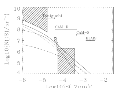
Figure 5: 6.7 $\mu$m source counts from HDF (central hatched regions). Models based on Franceschini et al. (1994): all components solid; spiral galaxies dotted; E+s0 dot-dash; AGN-dash. Faint end upper limits (hatched) come from the $P(D)$ analysis. The depths probed by other, forthcoming ISO surveys are indicated (ELAIS: Oliver et al. 1997; CAM-D & CAM-S: e.g. Elbaz 1997; Taniguchi: Taniguchi et al. 1997)

Figure 6: 15 $\mu$m source counts from HDF (central hatched regions) with IRAS 12 $\mu$m counts (thick line) at bright end, from this paper and Rush et al. 1993 (IRAS data shifted to 15 $\mu$m using cirrus spectrum). Models based on Franceschini et al. (1994): all components solid; spiral galaxies dotted; star-bursts dash-dot-dot-dot; s0 dot-dash; AGN-dash Elliptical galaxies-short dashes. Faint end constraints (hatched) come from the $P(D)$ analysis. The depths probed by other, forthcoming ISO surveys are indicated (ELAIS: Oliver et al. 1997; CAM-D & CAM-S: e.g. Elbaz 1997)

4.4 Comparison of Models

Table 2: Expected number of sources in ISO HDF Survey above 38.6$\mu$Jy at 6.7 $\mu$m, taking into account the areal sensitivity in Figure 1 using the PRR model. The number of associated sources observed above this flux limit was 5. For the simulation we did not exclude the one non-associated source above our flux limit since the simulation accounts for spurious sources. The second column indicates the number of sources expected at fluxes brighter than our brightest source. The final column is the probability of the observed fluxes being drawn from the model distribution, estimated using a K-S test

Component	$N$	$N$	K-S
	$(S>38.6\mu\rm{Jy})$	$(S>65.7\mu\rm{Jy})$	/%
Normal:	3.13	2.27	0.44
Star-bursts:	1.27	0.92	0.48
Seyfert 1:	0.66	0.44	1.30
Seyfert 2:	0.60	0.42	0.59
Total:	5.67	3.95	0.53
Simulation:	4.37	2.86	0.73

Table 3: Expected number of sources in ISO HDF Survey above 38.6$\mu$Jy at 6.7 $\mu$m, taking into account the areal sensitivity in Figure 1 using the AF model. The number of sources observed above this flux limit was 5. The second column indicates the number of sources expected at fluxes brighter than our brightest source. The final column is the probability of the observed fluxes being drawn from the model distribution, estimated using a K-S test

Component	$N$	$N$	K-S
	$(S>38.6\mu\rm{Jy})$	$(S>65.7\mu\rm{Jy})$	/%
Spiral:	1.33	0.78	3.56
Elliptical/S0:	2.10	0.98	15.78
AGN:	0.34	0.26	0.21
Total:	3.77	2.03	6.87

Table 4: Expected number of sources in ISO HDF Survey above 255$\mu$Jy at 15 $\mu$m, taking into account the areal sensitivity in Figure 2 using the PRR. The number of associated sources observed above this flux limit was 11. For the simulation we did not exclude the five non-associated source above our flux limit since the simulation accounts for spurious sources. The second column indicates the number of sources expected at fluxes brighter than our brightest source. The final column is the probability of the observed fluxes being drawn from the model distribution, estimated using a K-S test

Component	$N$	$N$	K-S
	$(S>255\mu\rm{Jy})$	$(S>726\mu\rm{Jy})$	/%
Normal	2.71	0.94	4.22
Star-bursts	2.81	0.89	5.83
Seyfert 1	0.73	0.22	9.00
Seyfert 2	0.78	0.26	4.57
Total	7.03	2.32	5.26
Simulation	8.37	1.88	2.31

Table 5: Expected number of sources in ISO HDF Survey above 255$\mu$Jy at 15 $\mu$m, taking into account the areal sensitivity in Figure 2 using the AF model. The number of sources observed above this flux limit was 11. The second column indicates the number of sources expected at fluxes brighter than our brightest source. The final column is the probability of the observed fluxes being drawn from the model distribution, estimated using a K-S test

Component	$N$	$N$	K-S
	$(S>255\mu\rm{Jy})$	$(S>726\mu\rm{Jy})$	/%
Spiral:	4.55	1.59	3.57
Star-burst:	1.26	0.52	1.25
Elliptical:	0.03	0.01	47.21
S0:	0.77	0.13	56.45
AGN:	0.25	0.07	14.93
Total:	6.87	2.33	4.76

Using the area of the survey to a given flux limit (Figures 1 and 2) and the number count models of Section 4.2 we can estimate the number of sources of any given type that we would expect in this survey, these numbers are summarised in Tables 2,4,3,5. Both models are consistent with the total number of associated galaxies. The simulation at 15 $\mu$m predicts that there should be 8.37 objects but our non-associated list includes 16 galaxies. This is a marginally significant excess and may indicate that either our association requirements are too harsh or that our simulated noise is not realistic; improved understanding of the ISO data in the near future will clarify this. Interestingly the PRR model predicts a significant fraction of objects ($\sim 70$ per cent) of the objects should be at fluxes brighter than our brightest source. This discrepancy is also seen in the integral count plots (Figure  3), where we can also see a apparent difference in slope between the model and the data.

To test whether discrepancies in the count slope are significant we perform a K-S test to assess the probability of the observed fluxes being drawn from a count distribution with the same shape as the models (or single components of the models), these probabilities are given in Tables2,4,3,5. These results suggest that the PRR model at 6.7 $\mu$m is ruled out with more than 99 per cent significance (using either the simulations or raw models), this is mainly due to the expected fraction of bright objects. This model cannot be ruled out with more than 95 per cent confidence at the other wavelength although the simulation implies a more significant discrepancy, this may again suggest problems with our simulations or association criteria.

In this test the AF model can also not be rejected with any high level of confidence (more than around 95 percent) at either wavelength.

It thus appears that these data are insufficient to rule out either model at 15 $\mu$m. The PRR model can be ruled out at the shorter wavelength due to the high fraction of bright galaxies predicted. It may be that revisions to the K-corrections of the “normal” component using improved SEDs may be sufficient to improve this model. Possibly problems with the “normal” component SED are also suggested by the noticeable over-prediction of the IRAS 15 $\mu$m counts in the model.

A “no evolution” version of the PRR star-burst component would predict only 0.28 galaxies 15 $\mu$m i.e. 4.5 in total. Since we comfortably detect 11 galaxies such a model can be ruled out at the 3 $\sigma$ level on integral counts alone.

5 $P(D)$ Analysis

Since our maps are close to the ISO confusion limit it is sensible to examine the low level fluctuations in the maps on a statistical level. This allows us to investigate source count models below the flux level at which individual sources can be resolved. To this end we explore the distribution of deviations in flux in a given aperture from the mean level, the $P(D)$ distribution. This analysis avoids the need for any source detection algorithm. The fluctuations in a map about the mean intensity consist of two components. The first is the noise which will have both positive and negative values, and will have some distribution function which we shall assume is Gaussian. The second is true fluctuations. These might arise from sources, cosmological background or Galactic foreground. In all cases this contribution will always be positive and thus skew a symmetric noise distribution. In this case we assume that any major asymmetric component arises from extra-galactic sources.

Firstly we select sky regions and construct a histogram of flux deviations in square apertures. These histograms are fitted with both Gaussian distributions functions and the expected distribution functions from the source count models. These model distribution functions are calculated following Franceschini et al. (1989) and using the AF model for the source counts discussed above (the differential counts of this model are similar to those from the PRR model below the source detection limit so the AF model results will be similar for both, and the model provides a better fit to the count distribution at 6.7 $\mu$m). The differential count distribution is first convolved with a model PSF (in this case a Gaussian PSF is assumed) to give the response function to single sources in the selected aperture. The $P(D)$ can then be calculated assuming the sources are distributed on the sky as a Poisson process.

Figure 7 shows the deflection distribution ($D$ in $\mu$Jy) obtained from a 72x72 matrix of pixels derived from the inner portion of the drizzled mosaic of Paper I. We estimate a sky standard deviation in the inner map outside obvious sources of $\sigma=16-17\mu$Jy/aperture. (dotted line in the Figure 7). The aperture is 6x6 arcsec² area, enclosing a disc with diameter equal to the FWHM of the theoretical PSF. The mean intensity was 0.4 mJy arcsec^-2.

The continuous thick line is the convolution of the Gaussian noise with a model $P(D)$ based on the counts appearing in Figure 6. The convolved curve provides a very good fit to the data (reduced $\chi^{2}\sim 1$). A simple Gaussian cannot fit the data, even if the width is increased to $\sigma=18-19\mu$Jy aperture^-1 with reduced $\chi^{2}>1.5$. Thus there is a clear positive signal in the $P(D)$. This means that the background in an extremely deep ISO exposure at $15\mu$m is structured. Such structure is entirely consistent with being due to an smooth extrapolation of the ISO source counts observed above the flux threshold, and confirms the counts.

This $P(D)$ analysis allows us to further constrain the models. The shape of the AF model counts was fixed and the normalisation allowed to vary. These constraints are illustrated in Figure 6

A similar analysis at 6.7 $\mu$m demonstrated that a simple Gaussian noise model was sufficient to provide a good fit to the observed $P(D)$. This allowed only an upper limit on the normalisation of the counts to be determined.

Figure 7: $P(D)$ analysis at 15 $\mu$m (see text)

6 Discussion of Populations

So far we have not made any use of the fact that our survey was conducted in the Hubble Deep Field and Flanking Fields where there is exceptional photometric and spectroscopy information available. These data allows us to determine the populations detected by ISO. It is still instructive to compare observed and predicted populations as this may provide clues for improvements to the models.

One of the 6.7 $\mu$m sources (ISOHDF2 J123646.4+621406) selected at 6.7 $\mu$m has broad emission lines (Paper IV). This is compatible with the predicted numbers of AGN in both of the models we have considered. Of the remaining 4 associated objects only one is compatible with a normal cirrus spectrum galaxy and has an elliptical morphology, the others are better fitted with star-burst spectra and have spiral morphologies (Paper V).

Excluding AGN, the first of the models (PRR) suggests that at 6.7 $\mu$m our sample should have a majority (71 per cent) of normal spiral galaxies with around 28 per cent star-burst galaxies. The expected probability of getting the observed one or fewer cirrus galaxies in a sample of 4 is $\sim 7$ per cent. Although the statistics are very poor this casts further doubt on the validity of PRR model at this wavelength. The classification of SEDs in Paper V is based mainly on the optical/IR luminosities. Extra information comes from the expected redshift distribution of these normal galaxies and star-bursts which is shown in Figure 8. A K-S test cannot rule out the possibility that the observed redshifts are drawn from the model distribution even if the redshift of the broad lined object is included: the probability of the data being drawn from the model distribution is 0.18.

Figure 8: Expected redshift distribution at 6.7 $\mu$m within the ISO HDF areas (accounting for the area dependent flux limit) for the star-burst and cirrus component of the PRR model. Over-plotted at arbitrary $y$ position are the redshifts (photometric or spectroscopic) for the 5 objects with reliable associations in Paper IV. The object at a redshift of 0.96 has broad lines in the optical spectrum. The probability that these data are drawn from the expected distribution estimated using the K-S test is 0.54 or 018 if the broad-lined object is included.

Figure 9: Expected redshift distribution at 15 $\mu$m within the ISO HDF areas (accounting for the area dependent flux limit) for the star-burst and cirrus component of the PRR model. Over-plotted at arbitrary $y$ position are the redshifts for the 6 objects with reliable associations and spectroscopic or photometric redshifts in Paper IV, the lowest redshift object has the lowest flux and was excluded from our count analysis. The probability that these data are drawn from the expected distribution estimated using the K-S test is 0.41, excluding the lowest $z$ object.

Paper V does not attempt to fit SEDs of the type used for the second model. However, this model predicts that the non-AGN 6.7 $\mu$m sources would be 61 per cent elliptical or S0 and 39 per cent spirals. This is reasonably consistent with the morphologies and SEDs above.

Only three of the 15 $\mu$m selected sources are associated within the HDF itself. Two of these have spiral morphologies and are fitted by star-burst spectra, while the third has elliptical morphology and a cirrus spectrum. With such limited statistics this is reasonably compatible with both models. Including the Flanking Field areas we find in Paper IV that six of the 15 $\mu$m selected sources have associations and redshifts (or photometric redshifts). These are shown in Figure 9 together with the redshift distribution from the PRR model. Excluding the lowest redshift object, (which was excluded from our count analysis as being below the 255mJy flux limit that was also applied to our model redshift distributions) we find that we cannot rule out these redshifts being drawn from this expected distribution (probability 0.41). This test is hampered by small number statistics but also assumes that the objects in the flanking fields with redshifts are not biased in any way. Clearly obtaining spectra for the flanking field 15 $\mu$m sources is a high priority.

7 Implications for Future Surveys and Missions

The fact that we have reached the ISO confusion limit at 15 $\mu$ms with a sensitivity of around 0.2 mJy has important implications for other surveys and missions, in particular NASA’s Small Explorer Mission, the Wide-Field Infrared Explorer (WIRE, http://www.ipac.caltech.edu/wire/). WIRE is due for launch in September 1998 and plans to survey hundreds of square degrees at 12 and 25 $\mu$m. The WIRE strategy is divided into three parts: Part I – a moderate-depth survey (60 percent of survey time); Part II – a deep, confusion-limited survey (30 per cent of the survey time) and Part III – an ultra-deep, confusion-distribution measurement. The areal coverage and integration times will be designed to achieve these aims and so the best estimate of the confusion limit is required prior to planning. Currently the WIRE team estimate confusion limits of between 0.067 mJy and 0.15 mJy at 12 $\mu$m (http://www.ipac.caltech.edu/WIRE/sensitiv.html) depending on the evolutionary models. WIRE has a 30cm mirror with poorer resolution than ISO so our results suggest that the confusion limit for WIRE will be brighter than these estimates.

8 Conclusions

We have investigated the source counts of our ISO observations at 6.7 and 15 $\mu$m of the Hubble Deep Field. These are the deepest available in the mid to far infrared wave-bands, 3 decades fainter than IRAS at 15 $\mu$m and the first ever presentation of extra-galactic source counts at 6.7 $\mu$m. We reach 50$\mu$Jy over 5 arcmin² at 6.7 $\mu$m, at 15 $\mu$m we cover 5 arcmin² to a depth 200$\mu$Jy and around 15 arcmin² to 400 $\mu$Jy. In both bands we cover smaller areas to deeper flux limits. These data will be very useful reference points for ongoing ISO surveys e.g ELAIS (see e.g. Oliver et al. 1997), the CAM Deep Survey (see e.g. Elbaz 1997) and the survey of Taniguchi et al. (1997). Both the source counts and a $P(D)$ analysis indicate that we have reached the confusion limit of ISO at 15 $\mu$m. This will have important implications for the construction of mid-infrared surveys with future space missions such as WIRE. At 6.7 $\mu$m we are close to the confusion limit but have not yet reached it. At 15 $\mu$m a no-evolution model is ruled out at $>3\sigma$ providing important confirmation of the strong evolution seen in IRAS surveys at a much greater depth. The counts appear to be steeper than expected from one a priori galaxy evolution model at 6.7 $\mu$m although the significance of this is dependent on our assumptions about the calibration and noise properties of the data and the FIR SED of the model which will improve with time. The $P(D)$ analysis provides constraints on number count models below the level at which we can extract reliable source lists.

Further information on the ISOHDF project can be found on the ISOHDF WWW pages: see http://artemis.ph.ic.ac.uk/hdf/.

Figure 10: $P(D)$ analysis at 15 $\mu$m (see text)

References

- [1] Bertin E., Dennefeld M., Moshir M. 1997, A&A (in press)
- [2] Eddington A.S., 1913, MNRAS, 73, 359
- [3] Elbaz D., 1997, in Laureijs R. & Levine D., eds ‘Taking ISO to the Limits’ (ESA)
- [4] Franceschini A., Mazzei P., De Zotti G, Giann F., Danese L., 1994, ApJ, 427, 140
- [5] Franceschini A., Toffolatti L., Mazzei P., Danese L., De Zotti G, 1991, A&AS, 89, 285
- [6] Franceschini A., Toffolatti L., Danese L., 1989, ApJ, 344, 35
- [7] Goldschmidt P. et al., 1996, MNRAS, this issue
- [8] Gregorich T.N., Neugerbauer G., Soifer B.T., Gunn J.E., Herter T.L., 1995, AJ 110, 259
- [9] Hacking P.B., Houck J.R., 1987, ApJS 63, 311
- [10] Lonsdale C.J., Hacking P. B., Conrow, T.P., 1990, ApJ, 358, 60
- [11] Mann R.G. et al., 1996, MNRAS, this issue
- [12] Oliver S.J., Rowan-Robinson M., Saunders W., 1992, MNRAS, 256, 15p
- [13] Oliver S.J. et al. 1997, in McLean B. et al. eds, Proc. IAU Symp. 179, New Horizons from Multi-Wavelength Sky Surveys, Kluwer, Dordrecht, in press
- [14] Oliver S., et al. 1995. In Proc. 35th Herstmonceux Conf. ‘Wide-Field Spectroscopy and the Distant Universe’ eds. S.J. Maddox and A. Aragon-Salamanca. (World Scientific) p. 274
- [15] Pearson C., Rowan-Robinson, M., 1996, MNRAS 283, 174
- [16] Puget J-L., Abergel, A., Bernard J-P., Boulanger, F., Burton, W.B., Desert, F-X., Hartmann, D. 1996, A&A 308, L5
- [17] Rowan-Robinson M., Saunders W., Lawrence A., Leech K., 1991, MNRAS, 253, 485
- [18] Rush B., Malkan M A., Spinoglio L., 1993 ApJS 89, 1
- [19] Serjeant S. el al., 1996, MNRAS, this issue
- [20] Saunders W., Rowan-Robinson M., Lawrence A., Efstathiou, G., Kaiser N., Ellis R.S., Frenk C.S., 1990, MNRAS, 242, 318
- [21] Taniguichi Y., et al 1997, in Laureijs R. & Levine D., eds ‘Taking ISO to the Limits’ (ESA)
- [22] Williams R.E. et al., 1996, AJ, 112, 1335