A Digital Photometric Survey of the Magellanic Clouds: First Results From One Million Stars1
Abstract
We present the first results from, and a complete description of, our ongoing digital photometric survey of the Magellanic Clouds. In particular, we discuss the photometric quality and automated reduction of a CCD survey (magnitude limits, completeness, and astrometric accuracy) that covers the central of the Large Magellanic Cloud (LMC) and of the Small Magellanic Cloud (SMC). We discuss photometry of over 1 million stars from the initial survey observations (an area northwest of the LMC bar covering ) and present a deep stellar cluster catalog that contains about 45% more clusters than previously identified within this region. Of the 68 clusters found, only 12 are also identified as concentrations of “old”, red clump stars. Furthermore, only three clusters are identified solely on the basis of a concentration of red clump stars, rather than as a concentration of luminous () main sequence stars. Extrapolating from the current data, we expect to obtain and photometry for 25 million stars, and and photometry for 10 and 20 million stars, respectively, over the entire survey area.
1 Lick Bulletin No. 1363
1 Introduction
Our knowledge of galaxies and stellar populations rests in large part on our understanding of the Large and Small Magellanic Clouds (LMC and SMC). Due to their proximity (49 and 57 kpc respectively, Feast & Walker 1987), relatively low line-of-sight extinction (Schwering and Israel 1991; Oestreicher & Schmidt-Kaler 1996), range of stellar populations (cf. Olszewski, Suntzeff, & Mateo 1996), various interstellar gaseous environments, and difference in mean metallicity relative to each other and to the Milky Way (Lequeux et al. 1979), these two galaxies are our most promising targets for detailed studies of galaxy evolution. Although the Clouds’ proximity allows us to resolve individual stars well down the luminosity function even in ground-based images, the Clouds have such a large angular extent on the sky that they are difficult to observe in their entirety. Investigations are generally limited to small, well-chosen regions, to low spatial resolution, or to shallow magnitude limits. For example, even the ambitious photographic surveys of the Clouds (cf. Hodge & Wright 1967; Hatzidimitriou, Hawkins & Gyldenkerne 1989), are either not very sensitive (Hodge & Wright’s plates have an average limiting magnitude of 17) or lack resolution (Gardiner & Hatzidimitriou’s (1992) COSMOS digitized scans of the ESO/SERC plates reach , but the authors confine their analysis to an area outside the SMC’s main body, the central 3∘ by 4∘, due to crowding). Furthermore, these and other large-area surveys, including the ongoing MACHO survey (Alcock et al. 1996), are conducted with only two optical filters, which limits the baseline for extinction measurements and the study of the full range of stellar spectral types. A photometric survey of the Magellanic Clouds that spans the full optical wavelength range will enable us to better understand our nearest galactic neighbors and provide a stepping-stone for future, focused investigations.
The development of large CCD arrays and a drift-scan camera (Zaritsky, Shectman, & Bredthauer 1996) that can scan at the extreme southerly declination of the Clouds (70∘) enables us to conduct efficiently a large-area, high-resolution, digital, multi-color photometric survey of the Clouds. Our goal is to image the central 8∘ by 8∘ of the LMC and 4∘ by 4∘ of the SMC in the bandpasses. We report on our initial observations, data reduction, and data analysis of a smaller ( 2∘ by 1.5∘) area of the LMC, and discuss the photometric and astrometric quality of the data in §2. In §3, we illustrate the usefulness of digital data by automatically identifying stellar clusters in the LMC from a stellar density image. Using a simple unsharp masking technique, we increase the number of known clusters in this region by about 45%. Other results obtained from these data will be reported elsewhere: for example, the reddening properties and constraints on the distribution of dust are described by Harris, Zaritsky, & Thompson (1997).
2 Observations and Data Reduction
The observations for this survey are to be obtained from a multiyear effort based at the Las Campanas 1-m Swope telescope using the Great Circle Camera (GCC; Zaritsky, Shectman, & Bredthauer 1996) and a thinned 20482048 CCD. The GCC enables us to drift scan at the declination of the Magellanic Clouds with minimum image distortion by rotating and translating a stage onto which the CCD dewar is mounted. The telescope remains parked during an exposure, but the CCD moves in such a way that a scan is performed along a great circle on the sky, rather than on a polar circle of constant declination. Implementing the motion requires an accurate rotational alignment of the camera and a precise measurement of the plate scale (both in terms of pixels per arcsec and in terms of stage movement per arcsec). Details of the scan geometry and camera are discussed by Zaritsky, Shectman, and Bredthauer. The effective exposure time is fixed by the time required for the sky to drift across the field-of-view of the stationary telescope (about 240 sec at the declination of the Clouds). Photometric standard stars are observed in a similar manner, which ensures that they have a well defined exposure time (the GCC does not have a precise shutter).
The two Clouds are divided into scan-sized sections, where each scan is about 2∘ long and 24 arcmin wide. Such scans take about 25 min to complete. The 8∘ by 8∘ LMC area is divided into 4 such scans in RA and 23 in Dec. The scans overlap by about 30 arcsec in right ascension and declination, which enables us to tie together the photometric and astrometric solutions. The CCD has a 0.7 arcsec pixel-1 scale and the typical seeing at the telescope is between 1.2 and 1.8 arcsec. When the survey progresses and the seeing statistics are better determined, we will select an upper limit on the seeing for acceptable data. Scan quality will be judged after reduction and unsatisfactory scans will be reobserved in subsequent observing runs.
In this paper, we present results from the LMC scans numbered 58, 62, 66, and 70, for which the start (westernmost) coordinates are listed in Table 1. These data were obtained during Nov 13-23, 1995. The box in Figure 1 outlines the area observed and numbers the scans, superposed on a greyscale image of the central portion of the LMC. When complete, the survey will cover a larger area of the LMC than that covered by the Figure. The data consist of Johnson , Harris , and Johnson exposures taken mostly in photometric conditions. Scans taken in moderately non-photometric conditions (e.g., slight cirrus) are corrected using the overlap regions with photometric scans. Details of the photometric matching of scans are presented in §2.1. The region observed was selected to provide a compromise in the level of stellar crowding and to avoid regions of high nebulosity. Regions with high stellar density and nebulosity will be observed as part of the complete survey.
2.1 Reduction Procedure
The quantity of data generated in this survey mandates that we automate the reduction. We constructed an algorithm that subtracts the bias using the overscan columns, “flattens” the image (along columns) using a drift scan of the twilight sky, fixes bad columns (which are defined by the user and are stable during a run) via interpolation, and divides each scan into twenty manageable sections ( pixels) that overlap each other by about 50 pixels. We refer to the small working images as subscans and each scan is divided into a 10 by 2 array of subscans. The photometry is obtained using DAOPHOT II (cf. Stetson 1987 for a description of the original DAOPHOT package; the version we use dates from April 1991) and coordinate solutions are derived using the Magellanic Catalogue of Stars (MACS; Tucholke, de Boer, & Seitter 1996). The photometric catalogs constructed from different subscans, and then from different scans, are pasted together to produce a final, uniform catalog. Details of this procedure are discussed next.
Crowded field stellar photometry is nearly an art form, but has become relatively standardized in great part due to the availability of the DAOPHOT suite of data analysis routines. We iteratively selected values for the appropriate parameters and developed an algorithm, using the DAOPHOT II routines, that minimizes the residuals in the star-subtracted image. Basically, we iterate three times through the reduction of every subscan to find a suitable point-spread function (PSF) and measure PSF photometry. The first pass is done using only a subset of the brightest stars (V 18.5) and an analytic Moffat function as the PSF model (a 2-D elliptical with an unspecified position angle). The stars used to derive the PSF are chosen from among the brightest non-saturated stars and then ranked in order of contamination by nearby neighbors. We use up to 100 relatively isolated stars that are at least 30 pixels from the image edge, within 4.5 magnitudes of the brightest non-saturated star (effectively, ), and in regions where the mean background sky is less than 1 larger than the mean sky in the image (to avoid regions with strong nebulosity). Once the sample of PSF stars is defined, it is used through the three iterations. In each iteration, nearby neighboring stars identified in the previous pass are subtracted before the PSF is calculated. The second pass is done using the same PSF model, but adding an empirical lookup table for deviations from the analytic form. The final pass is done with a spatially quadratically variable Moffat function plus an analytic lookup table.
The PSF can vary along the length of a scan, either because the GCC motion is not entirely compensating for field motion (as can happen if the stage alignment is not quite perfect), or because the seeing changes with time. However, we find that the PSF in sections of about 1000 pixels square is well-behaved (e.g., it can be modeled with a spatially quadratically variable function without leaving significant positional dependent residuals in the star subtracted image). This finding and the issue of image manageability dictate that the reduction be done on subscans of roughly 1000 pixels on a side. We present data from the first (westward) 9/10ths of each scan because the scans are systematically poor at the scan end (the last 1/10th of the scan). This “tracking” problem has since been corrected, but we exclude the poor quality data from further discussion.
The result of executing the above procedure is a list of positions and instrumental magnitudes that are based on the amplitude of the best-fit PSF for each star. Aperture corrections, which convert that magnitude into an instrumental total magnitude, are computed using images from which all stars, except those used to derive the PSF, are subtracted. The aperture correction is calculated by evaluating the magnitude of every PSF star in concentric apertures of increasing radius and extrapolating the magnitude vs. aperture size relationship to infinite radius. The correction is applied to all stellar magnitudes from the relevant subscan. Any errors in aperture corrections will become evident when comparing photometry from overlapping subscans.
To match the photometry for stars in one subscan either to those of adjacent subscans in the same filter or to overlapping subscans in other filters, we need to convert the stellar positions into equatorial coordinates. Subscans and scans cannot simply be registered and combined because the geometric transformation between pixel and equatorial coordinates depends on the motion of the GCC and can be slightly different even for scans of the same region. For example, the plate scale, and therefore the CCD readout rate, changes among filters. To convert between positions and equatorial coordinates, we utilize the Magellanic Catalogue of Stars (MACS; Tucholke, de Boer, & Seitter 1996). We minimize the residuals between the coordinates of astrometric standards from the MACS and those derived for the same stars from a gnomic-projection of the equatorial coordinates onto our -space. We typically match between 20 and 40 MACS stars per subscan from which we define the plate solution. This procedure enables us to derive the scale, orientation, and central coordinates of each subscan. We use these solutions to convert the positions of all stars to RA and Dec. The rms differences among the cataloged and measured positions from our frames is typically 0.3 to 0.4 arcsec (cf. §2.3.2 for more details).
Using the equatorial coordinates, we combine the stellar lists from the matching subscans to produce a list that includes coordinates and magnitudes for the stars in all four filters. The data are adopted as the positional reference. Data from other filters are matched to the data. We match stars in two different filters by using a search radius equal to twice the rms positional scatter of the worst astrometric solution for the two relevant subscans. The nearest star in the frame being matched to each star in the frame that is within the search radius is adopted as the matching star. After completing the first attempt at matching all of the stars between the two subscans, we apply a positional offset to the data from the second frame (no scale change or rotation is allowed) so that the mean positions of the matched stars in the second subscan agree with those of the matched stars in the subscan. Next, we increase the search radius by 0s.1 and redo the search. We continue incrementing the search radius by 0s.1 until the former iteration produced at least 99% of the matches found in the latter iteration. We repeat this procedure with the photometry from each filter relative to data. Unmatched stars are retained in the catalog at this point. The scans in different filters do not overlap precisely, so some stars identified near the image edge in one filter may lie on a different scan or subscan. Retaining stars that are found in only one filter enables us to recover their matching stars when different subscans are matched. This procedure results in lists of equatorial coordinates and four-filter photometry corresponding to each subscan.
The data from each subscan are combined with those from the adjacent subscans in RA by iterating using the same matching algorithm. In this case, we begin with a matching radius of 0s.4 and increment the search radius by 0s.1 until subsequent searches identify the same number of matches to within 1%. If the mean positional offset between subscans is greater than one-half of the standard deviation of the stellar positions, we recenter the subscans relative to each other and redo the matching. We average the magnitudes for matched stars. These are not two independent measurements of the magnitudes, because they are drawn from the same image, but the measurements do differ slightly due to the different derived PSFs and aperture corrections. No mean magnitude offsets between subscans are applied (the corrections were found to be too unstable and caused the photometry along a scan to random walk). We repeat this procedure until each of the two sets of nine subscans, for each scan, are matched in RA. We then match the two sets in Dec following the same procedure. As mentioned above, because we retain stars that are observed in at least one filter, we do not lose stars because of slight misalignments between scans. Once all of the subscans from one scan are combined, then the photometric calibration (see below) is applied to the data from that scan. Finally, we only retain stars for which at least and measurements are available in order to minimize spurious detections.
The data from the various full scans are matched to each other only after the photometric calibration so that all scans are on the same photometric system when combined. The stars in overlapping scans are matched using the same algorithm that was used to match stars in overlapping subscans, except that we now apply a magnitude correction between scans because different scans may have slight zero-point magnitude differences. Several hundred (for the frames) to several thousand (for the frames) stars are typically matched in the overlap regions between scans. Data for each filter are matched independently. In the simplest case, a single constant magnitude offset between scans would suffice. However, we find that there are slight, but systematic, variations along scans. If severe ( mag), these fluctuations are possibly an indication of nonphotometric conditions; if slight, these are possibly due to changes in the PSF and the related aperture correction. In either case, we need to map and remove the relative variations between scans using a fiducial scan that is thought to be free of temporal magnitude variations. We choose to reference all of the scans to scan 62, which has high-quality images taken in photometric conditions for all filters and includes an OB association with previously published photometry for comparison.
The procedure for mapping the magnitude variations between scans is described next. We fit a 5th order (for the frames) or 10th order polynomial to the magnitude differences between matched stars versus RA (only using magnitude differences that are within of the mean difference). The fitted polynomial describes the mean photometric offset between the two scans as a function of RA. The typical corrections have small spatial variation and zero-point photometric corrections 0.1 mag (cf. Figure 2). One particular scan (70 in ), taken during nonphotometric conditions, shows fairly large photometric variations along the scan. The polynomial fits are used to reference the photometry from the three other scans to that from scan 62. For a small section of scan 62, we can check our photometry with published photometry (see discussion in §2.4). Eventually, our observations will extend over an area that is roughly 25 times the current area and will overlap with a variety of published photometry. Comparison with those data will confirm the overall photometry and whether the scans were properly referenced to each other.
2.2 Standards
The photometry is calibrated to the Landolt system (Landolt 1992). The details of the standard star reductions, repeatability, and color terms are discussed below. The photometric calibration is fairly standard and done within DAOPHOT. We solve for , , , and color terms for , , , and , respectively, and for extinction as a function of airmass, . The equations solved are
where is the zero point in the respective filter, is the color term, is the extinction coefficient, and the primed magnitudes are instrumental. We list the best fit coefficients, observational scatter, and number of stars used in the fits in Table 2. Data for each color come from two separate nights. We find no significant variation between nights, so we combine the data in order to best determine the zero point and color terms. The scatter introduced by the calibration is fairly small, 1 to 3%.
2.3 Internally Estimated Uncertainties
2.3.1 Photometry
To determine the stability of the DAOPHOT photometry, we compare the photometry for a set of stars in the overlap regions between scans or subscans. One concern is that the photometry may vary between scans or within a scan due to PSF variations. The best available internal test comes from the comparison of adjacent scans. Adjacent scans are typically from different nights and so have different seeing, extinction, and focus, as well as completely independent reduction.
The internal photometric stability can be demonstrated in at least two ways. First, the absence of any obvious discontinuities in the magnitude differences for stars observed in scan overlap regions, plotted in Figure 2, argues that the reduction of subscan images is stable. There is no evidence in Figure 2 that photometry from different subscans varies significantly. Of all the scans, only scan 70 in appears to have serious photometric problems, but those are most likely the result of nonphotometric conditions. Second, the magnitude differences between matched stars are in rough agreement with the internally estimated uncertainties. In Figure 3, we present the uncertainty normalized differences between magnitudes in the two scans after the polynomial photometric offset is applied. If the propagated uncertainties are a true and complete reflection of the uncertainties (excluding uncertainties in the photometric calibration), these histograms should approach a Gaussian with a dispersion of one. We plot such Gaussian curves for comparison. In most cases, the propagated uncertainties only moderately underestimate (0 to 40%) the true internal uncertainties. The values of the quantity
are given in Table 3, where represents the degrees of freedom in the fitted polynomial, the number of stellar pairs, and the magnitudes for the given star in each of the two scans, and the propagated uncertainty in the magnitude error. Including scan 70, the values of suggest that the uncertainties are underestimated by a factor 2, and are typically underestimated by less than a factor of 1.5.
We conclude that scientific results that are robust to a factor of two change in the current uncertainties are trustworthy. Eventually, with additional scans, we will be able to ascertain whether the true uncertainty is up to a factor of two larger than estimated by propagation of DAOPHOT error estimates, or whether a subset of the scans (e.g., scan 70) should be observed again.
2.3.2 Astrometry
We estimate the astrometric precision by examining the distribution of rms residuals between our coordinates and the cataloged positions of the MACS stars among the subscans. In Figure 4, we plot a histogram of the residuals in the astrometric solutions of all of our 72 subscans. The mean rms scatter is below half an arcsec. The positional uncertainty of the MACS stars is moderate (generally 0s.5; Tucholke, de Boer, & Seitter). Given our range of rms residuals, we do not appear to be introducing significant uncertainties from the application of our gnomic-projection coordinate transformation.
The matching of subscans and scans, which uses data from the edges of subscans and scans, places the strictest demands on the coordinate solutions. If stars at the edge of subscans have significantly larger astrometric errors, then fewer stars will be matched along subscan edges than in the middle. Such a trend is not observed (see below). On the other hand, if the stars at the edges of entire scans have significantly higher astrometric errors, then observations of the same stars in overlapping scans would not be matched and those stars would appear twice in the catalog. We find that if we adopt a search radius of 3 times the rms scatter of the astrometric standards (a typical radius of about 1s.2) for subscan or scan matching, we see no significant spatial variation that correlate with the edges of the subscans or scans in the number of stars in the final catalog for stars with (737,840 stars). We do see such variations for a choice of a matching radius of two times the positional difference, suggesting that some positions at the edges of the subscans may have errors 0s.8. As we discuss below, the completeness of the survey drops sharply at and since different scans, and even different subscans, can have different magnitude limits due to changes in the seeing and stellar density, there will be apparent discontinuous stellar density differences for stars with , even if the astrometric positions are accurate.
To qualitatively demonstrate the spatial uniformity of the final catalog, we produce a stellar density image of the catalog. We include all stars with , and bin the density image into 15 arcsec square pixels. This image is then smoothed with a Gaussian function with 2 pixels to bring out low signal features in the distribution. The use of the stellar density weights this image toward stars near the magnitude cutoff and so is most sensitive to spurious detections and mismatches. This stellar density image is shown in Figure 5. The union between subscans and between scans is nearly seamless (the principal blemish, the cross feature just north of the dominant stellar association in the field is due to a super-saturated star that contaminated the nearby photometry).
2.4 Externally Estimated Uncertainties
The most challenging test of the data is a comparison to previously published results by other investigators. Our direct comparison to published CCD photometry (Oey 1996) of the LH 38 region to a limit of is presented in Figure 6. We matched stars between our list and Oey’s list using the same algorithm employed to match the photometry from various scans with fixed search radius of 2s.0. We match 252 of 274 stars in Oey’s list in and and 103 of 111 in . The stars that are unmatched are generally in crowded regions and are either missing or identified at sufficiently different positions. Finally, we note that this region spans the edges of two of our scans, and so acts as a further test of the scan-matching algorithms.
The agreement between Oey’s photometric data and ours is generally excellent, despite the nebulosity and high stellar density in this region. The zero point deviations, including all matched stars that are within 3 of the one-to-one correspondence line, are 0.064, 0.049, and 0.039 magnitudes for , , and . Aside from the zero point deviations, there is a slight, systematic deviation at the bright end, especially in the filter (see lower panel of Figure 6). The deviation is of the sense that Oey’s photometry underestimates the magnitude relative to our measurement, possibly suggesting the onset of non-linearity in Oey’s data. This non-linearity is consistent with the appearance of the brightest stars in Oey’s images which show hints of diffraction spikes. In her comparison to previous work she obtained zero point magnitude offsets similar or larger than those discussed above, so that the offsets found between scan 62 and her data are entirely consistent with those found among previous investigators. Referencing our photometry to Oey’s in the mean, then the values from the one-to-one correspondence line between Oey’s data and ours, excluding outliers, are 1.93, 1.50, and 2.20, for , , and respectively. These measurements of the uncertainties are only slightly larger than the results we obtained from our comparison of overlapping scans. The histogram of uncertainty-normalized deviations between our data and Oey’s is shown in the upper panel of Figure 6.
The results of this comparison indicate that the photometry from the survey is reliable, although our propagated uncertainties appear to underestimate the true external error by a factor of 1.5 (excluding zero point uncertainties and attributing the majority of the outliers to incorrect matches). The random error is the principal uncertainty of interest because any zero point uncertainty will be reduced with time as our survey area increases and comparisons with more published photometry become possible.
2.5 Super-Saturated Foreground Stars
In a few instances, stars are sufficiently bright that their images in the CCD scans distort the photometry of objects in their vicinity. DAOPHOT identifies numerous spurious stars from fluctuations in the luminous halos of these stars. For a star to saturate so intensely it must have an apparent magnitude brighter than 10th magnitude. If such a star is in the LMC, then it would have an absolute magnitude brighter than 8.5 ( for a main sequence star), which is exceedingly rare (see Massey et al. 1995 for examples). Therefore, these heavily saturated stars are probably foreground stars. The photometry in the area surrounding these stars is most affected in the images. We automate the search for these super-saturated stars by making a color image of the stellar density using 1515 arcsec pixels. Because DAOPHOT tends to identify many spurious stars that are bright in around these problem stars, we search for regions of the density map that are anomalously red (or that have large ). We first median filter the image using a 2 by 2 pixel box to remove single luminous red stars. We then run SExtractor (Bertin & Arnouts 1996) to identify bright sources (selected to have at least 10 pixels that are at least 2 above the mean), which we compare interactively with the unfiltered image. We find 24 significant objects in the entire surveyed region. These objects are typically annuli in the density image, where the core is vacant because of saturation and the wings are densely populated due to spurious sources.
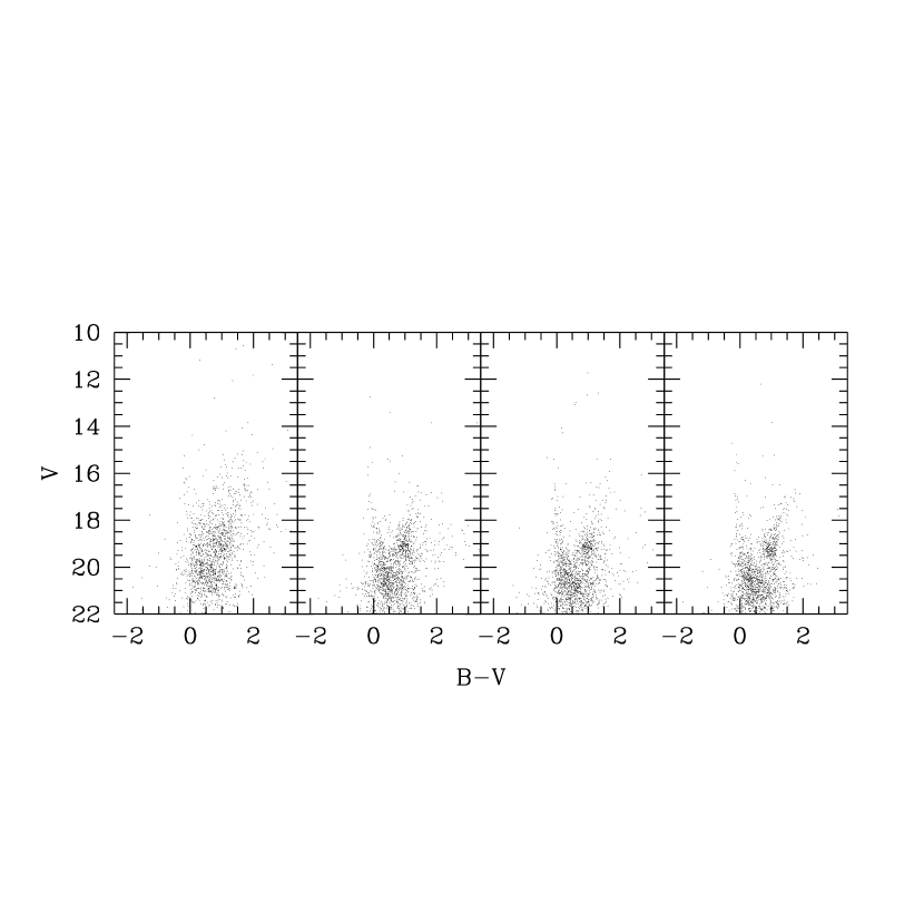
We mask these regions using the results from SExtractor and an interactive determination of the mask size that we describe next. The mask aperture should be related to the “luminosity” of the sum of spurious stars, so we use the SExtractor “magnitudes” to set a scale for the masks. We set the normalization interactively by considering a range of normalizations and examining the color-magnitude diagrams of stars identified within those mask apertures. In Figure 7, we plot those CMD diagrams, beginning with the core region (typically about 7 arcsec to 20 arcsec radius, depending on the SExtractor “luminosity”). Three larger annuli, each of which contains roughly the same number of stars as the inner annulus, are compared to the inner annulus. The effect of the saturated stars is especially evident in the inner region, even among and photometry where the effect is smaller than in . The upper main sequence and RGB clump tighten substantially for annuli far from the saturated stars. Conservatively, we will exclude a region around these saturated stars equal to the area covered by all of the panels in Figure 7, even though the last two panels appear to be undisturbed by the saturated star. The adopted mask apertures correspond to between 15 and 45 arcsec in radius. This cut excludes only a small fraction of the total number of stars, 3,753 out of 737,840.
2.6 Completeness
As is always the case in crowded-field photometry, some stars brighter than the detection limit are missed due to blending. We use the standard artificial star algorithm from DAOPHOT to add stars to the images at random and to estimate the completeness of our sample by attempting to recover these artificial stars. Five hundred stars over the full range of magnitudes are added at random to two subscans from each scan. We conduct five realizations, each with 500 artificial stars. Instrumental magnitudes are remeasured for all of the stars in the frame using the three-iteration DAOPHOT algorithm described previously. By determining which artificial stars are recovered, we estimate our completeness as a function of magnitude in each filter. In addition to identifying artificial stars as lost if no match is found, we also identify stars as lost if the magnitude of the matched star differs by more than 0.5 mag and if such a discrepancy is significant at the greater than 5 level. The general procedure of placing artificial stars at random within an image neglects any correlation in the stellar distribution, which is roughly valid for the overall survey, but grossly incorrect for stars in stellar clusters.
In Figure 8, we present the derived completeness fractions for two scans (58, which has the highest mean stellar density, and 66, which has the lowest stellar density among those observed in photometric conditions) as a function of magnitude. The Figure illustrates substantial incompleteness () occurs only for magnitudes fainter than 21 in and . In the Figure, we also include the magnitude at which the completeness fraction drops below 0.5. Among the mean stellar densities covered in our present survey, there are no large differences in completeness, with the possible exception of the band data. The slight differences between scans are a result of various effects, including different stellar densities, seeing, and a variable PSF. In general, we conclude that the survey is complete at the 50% level for ,.
Despite this general conclusion regarding completeness, a visual inspection of the stellar density image clearly shows that the incompleteness can be rather severe even for relative bright stars in the densest regions. For example, there is a clear absence of red clump stars () at the center of the richest clusters in the region surveyed. Therefore, completeness corrections should be calculated in detail for any analysis of the survey data that requires a complete stellar sample or detailed knowledge of the selection effects.
3 Discussion
The data obtained from this survey will be used to address a wide range of issues — from the study of the spatial variations in star formation history to identifying background quasars for study of the low density ISM. We are currently studying the extinction in this region (Harris, Zaritsky, & Thompson 1997) and the spatial distribution of stars.
The Hess diagram for this region of the LMC is shown in Figure 9. We construct this diagram by modeling each star with a Gaussian of width along each axis corresponding to its observational uncertainty along the axis. We sum the Gaussians and take the square root of the intensity in each pixel to enhance the contrast of the diagram in Figure 9. Data for over 1 million stars identified in both and are incorporated in this Figure. A complex star formation history is evident: both a significant upper main sequence and a red giant branch are visible. In the future, we will present a detailed analysis of the constraints imposed by these data on the star formation history.
3.1 LMC Clusters
One straightforward use of these data is to identify star clusters. Given the digital nature of the data, we can easily construct density maps that are independent of nebular emission and that utilize color and magnitude information. We have previously discussed the stellar density image shown in Figure 5. Each pixel is 15 arcsec on a side and the intensity of each pixel reflects the number of stars in that pixel that are in the catalog (i.e., stars identified in both and ). This map of the stellar density enables us to select clusters simply on the basis of stellar density rather than being biased by the presence of luminous stars. We only use stars with mag and apply no color criteria to generate Figure 5. We proceed by identifying significant concentrations of stars. We create one version of the density image that is smoothed using a Gaussian with 2.5 pixel width and another image smoothed with a Gaussian 3 times as wide (7.5 pixels). We then subtract the latter from the former to remove the smooth background and accentuate the clusters (i.e., unsharp masking). The image analysis package SExtractor (Bertin and Arnouts 1996) is used to identify significant objects in this image. Our objective is to maximize the number of objects detected, while minimizing spurious detections. For detection, we require than an object contain at least 5 significant pixels and we examine three choices for the threshold at which a pixel is considered significantly above the mean (3, 4, and 5). By applying our three choices of significance thresholds to the image, we identify 157, 78, and 45 objects, respectively. To determine the number of spurious detections in this procedure, we invert the image and search for positive detections. In the negative image, we find 31, 6, and 0 detections. Of the six detections found with the choice of a 4 significance threshold, five were adjacent to the two most significant clusters NGC 1846 and NGC 1851 and result from the dark halos generated by the unsharp masking process. Therefore, we conclude that the choice of 4 maximizes the number of detections, while keeping the number of false detections to fewer than one or two.
In Figure 10, we present the unsharp mask image used to identify clusters and our cross identification with objects in the Kontizas et al. atlas (1990). Objects marked SP are suspected to be spurious because they lie at the boundaries between scans or subscans, and because the density at those boundary regions can be nonuniform due to slight matching difficulties (the unsharp masking technique accentuates these boundaries). The objects marked AN (for anonymous) are identified as new clusters, for which no identified counterpart was available in the Kontizas et al. catalog. Objects marked Ce are clusters found in what was previously identified as an emission line region in the Hodge and Wright atlas (1961; from identifications by Henize 1956). Objects marked K are from the Kontizas et al. catalog. Within this region, we identify 38 of the 44 clusters in the Hodge and Wright atlas, 9 additional clusters found by Kontizas et al. , and 21 new clusters. Note that some of the clusters (eg. K 544 and K 622 were identified by Hodge (1988) as 131 and 188 respectively) and that AN 4 is close to, but not exactly at, the position of Hodge’s (1988) cluster 118. Table 4 lists the positions from our astrometry, the previous identification if available from the Kontizas et al. catalog, and a measure of the total stellar content of the clusters, , (log(stellar content)) for intercomparison between clusters. The richness measure, , is highly uncertain and biased low at the rich end due to crowding effects and saturation.
Why do we miss certain clusters (NGC 1873, HS 130, HS 208, HS 222, HS 225, and SL 289)? Some clusters, such as HS 130, are visible in the unsharp masked image, but they are insufficiently significant to be detected with our particular chosen detection parameters. We test whether the cluster contrast is higher for these particular clusters if either a brighter magnitude or bluer color criterion is imposed. If we use to generate the stellar density image, then we detect NGC 1873, HS 130, HS 208, and SL 289 from the list of previously missed clusters, but we lose HS 154, NGC 1911, NGC 1915, SL 263, and SL 269 as well as AN 2, 4, 9, 10, 11, 13, 15, and 17, presumably because these clusters have proportionally fewer luminous stars. If we set our criteria to include upper main sequence stars and exclude evolved stars, and , then we identify NGC 1873, HS 130, HS 208, and SL 289, but we lose NGC 1895 and AN 2, 5, 11, and 15. Finally, selecting clusters only on the basis of the density distribution of red clump stars, we find only 14 significant objects, two of which are on the very edge of the image and clearly unreliable. Therefore, in contrast to the 68 clusters identified using all of the stars, there are only 12 statistically significant concentrations of red clump stars. The detections correspond to NGC 1806, SL 174, AN 5, SL 298, NGC 1871, NGC 1852, NGC 1829, NGC 1846 (3 of the additional objects are unmatched objects and 1 is spurious). This list includes some of the richest clusters (e.g., NGC 1806, NGC 1846, SL 298, and NGC 1852), and so we suspect that these are detected only because they are so rich to begin with that a large concentration of red clump stars is found. The three clusters that are only detected on the basis of their red clump star concentrations may be more representative of the field stellar population. We will discuss the use of CMD diagrams to help further define the cluster star formation history of the Clouds elsewhere.
4 Summary
We discuss the first data from a, 4-band, CCD survey of the central 8∘ 8∘ of the LMC and 4∘ 4∘ of the SMC. We have developed an automated data reduction pipeline that utilizes DAOPHOT II to reduce drift scan images obtained using the Great Circle Camera at the Las Campanas 1-m Swope telescope. The photometric uncertainties, based on both internal and external comparisons of stellar magnitudes, are at most a factor of two worse than estimated from the internal, propagated uncertainties generated by DAOPHOT and the associated reduction pipeline. Although a comparison with published photometry can only currently be done for one region, LH 38 (Oey 1996), the photometry is consistent among the two studies. As our survey grows, there will be many overlapping regions available both to confirm the automated reduction and to accurately fix the photometric zero point. Astrometric precision appears to be roughly 0s.5 for most of the survey. Although astrometric and photometric accuracy is dependent on seeing, there are no large-scale variations in data quality over the observed area (with the exception of one scan taken in non-photometric conditions). Completeness is greater than 50% for and we identify some stars down to . The other bands are observed to comparable limits.
The data are not yet publically available because we expect that some slight modifications to the data reduction pipeline may be necessary after more data, especially in regions of higher stellar density, are obtained. Those interested in the data described here should contact the first author.
We search the data for previously undiscovered star clusters by examining the stellar density image of the region. We use unsharp masking techniques on various subsamples of the data to construct a cluster catalog that increases the number of identified clusters by about 45%. The use of the stellar density, particularly at magnitudes of , allows us to identify clusters that are not easily identified solely on the basis of the upper main sequence. Further study of these fainter clusters may help clarify the cluster star formation history in the LMC. We do not find a significant population of clusters with a large red clump stellar population (only three, in comparison to 68 clusters, might lack an upper main sequence and have a strong red clump population). This findings are consistent with a lack of intermediate age-relative metal rich clusters and the large numbers of young clusters (age 4 Gyr; e.g., Olszewski, Suntzeff, Mateo 1996 and references therein). Additional inferences await the detailed analysis of the cluster CMDs.
This paper describes the first steps toward a complete, digital, photometric, survey of the LMC and SMC. The quality of the survey is such that a variety of questions can be addressed with the data, ranging from the identification of star clusters, as done here, to more complicated issues regarding the structure and evolution of the Magellanic Clouds. In combination with an ongoing emission line survey (Smith et al. 1996) and other surveys of the Clouds, these data should provide new insight into our nearest galactic neighbors.
Acknowledgments: DZ gratefully acknowledges financial support from a NASA LTSA grant (NAG-5-3501) and an NSF grant (AST-9619576), support for the construction of the GCC from the Dudley Observatory through a Fullam award and a seed grant from the Univ. of California for support during the inception of this project. We thank A. Zabludoff for a comments on a preliminary draft. We also thank C. Anderson and S. Gibson for making available the image in Figure 1, originally obtained by Henize. DZ also thanks the Carnegie Institution for providing telescope access, shop time, and other support for this project, and the staff of the Las Campanas observatory, in particular Oscar Duhalde, for their usual excellent assistance.
References
Alcock, C. et al. 1996, ApJ, 461, 84
Bertin, E., & Arnouts, S. 1996, AA, 117, 393
Feast, M., & Walker, A.R. 1987, ARA & A, 2, 345
Gardiner, L.T., Hatzidimitriou, D. 1992, MNRAS, 257, 195
Harris, J., Zaritsky, D., & Thompson, I. 1997, in prep.
Hatzidimitriou, D., Hawkins, M.R.S., & Gyldenkerne, K. 1989, MNRAS, 241, 645
Henize, K.G. 1956, ApJS 2, 315
Hodge, P.W., & Wright, F.W. 1967, “The Large Magellanic Cloud”, (Smithsonian Press: Washington, D.C.)
Hodge, P.W. 1988, PASP, 100, 1051
Kontizas, M., Morgan, D.H., Hatzidimitriou, D., & Kontizas, E 1990, AA Sup., 84, 527
Landolt, A.U. 1992, AJ, 104, 340
Lequeux, J., Rayo, J.F., Serrano, A., Peimbert, M., & Torres-Peimbert, S. 1979, AA, 80, 155
Massey, P., Lang, C.C., DeGioia-Eastwood, K., & Garmany, C.D. 1995, ApJ, 438, 188
Oestreicher, M.O., & Schmidt-Kaler, T. 1996, Bull. Am. Astr. Soc., 117, 303
Oey, M.S. 1996, ApJS 104, 710
Olszewski, E.W., Suntzeff, N.B., & Mateo, M. 1996, ARA & A, 2, 511
Schwering, P.B.W., & Israel, F.P. 1991, AA, 246, 231
Smith, R.C., et al. 1996, BAAS, 188, 5101
Stetson, P.B. 1987, PASP, 99, 191
Tucholke, H.-J., de Boer, K.S., & Seitter, W.C. 1996, AA, 119, 91
Zaritsky, D., Shectman, S.A., & Bredthauer, G. 1994, PASP, 108, 104
Figure Captions
unavailable electronically
The area of the LMC observed in this work is shown as a box overlayed on an greyscale image of the LMC, with each scan numbered. North at the top, East to the left. The rectangular box subtends approximately 2∘ by 1.5∘.
The photometric matching of adjacent scans using stars common to both scans. The scan pair is labeled at the top of each column, and each column contains the comparison for each of the four filters. The solid line illustrates the polynomial fit used to register the photometry. Note that the scale is vertically shifted for the matching of scans 66-70 (labeled to the right of the plot).
The uncertainty-normalized magnitude differences for stars matched between different scans. The scan pair is labeled at the top of each column, and each column contains the comparison for each of the four filters. The solid curves are Gaussians with unit dispersion.
The distribution of astrometric differences between our gnomic-projection equatorial coordinates and those in the Magellanic Catalogue of Stars (Tucholke, de Boer, & Seitter 1996) catalog for all 72 scans.
available at http://www.ucolick.org/instruct/lmcdir/fig5.jpg
A stellar density plot (1 pixel = 15 arcsec) for all stars with . Corresponds the region of the four scans shown in Figure 1. North at the top, East to the left. The image is roughly 2∘ across.
Comparison between photometric data from Oey (1996) and the survey data. Lower panels contain differences in magnitudes as a function of magnitude. Solid lines indicate mean offsets in photometry. The panels are , , and data left to right. Upper panels show the distribution of magnitude errors normalized by the propagated internal uncertainty. The solid curve represents a Gaussian with . In the panel, the thinner line represents a Gaussian with .
The color-magnitude diagrams for regions around supersaturated stars. Each panel contains roughly the same number of stars in annuli of increasing radii. The effect on the photometry from the saturated stars is gross in the innermost section and negligible in the last two panels. We mask a region equivalent to the area encompassed by all four sections from further analysis.
Results from artificial star experiments. The completion fraction as a function of magnitude is shown for subscans of scans 58 and 66 for the four filter bandpasses. Included in each panel is the magnitude at which the completeness fraction drops below 0.5.
unavailable electronically
A Hess diagram (a density-weighted CMD) for and . The left panel shows the greyscale version of the square root of the stellar density (for the purpose of reducing contrast) across the color-magnitude plane, while the right shows a surface plot of the true density distribution to illustrate the relative number of stars in the various components.
unavailable electronically
An unsharp-masked image of the stellar distribution shown in Figure 5, with clusters labeled. Same region and orientation as in Figure 5. Objects labels are described in the text.
| Scan (2000.0) | ||||||
| 58 | 05 | 00 | 28 | 67 | 53 | 10 |
| 62 | 05 | 00 | 46 | 67 | 31 | 36 |
| 66 | 05 | 01 | 02 | 67 | 9 | 46 |
| 70 | 05 | 01 | 19 | 66 | 47 | 27 |
| Filter | A | B | C | ||
| 5.335 | 0.122 | 0.322 | 0.032 | 60 | |
| 3.557 | 0.070 | 0.234 | 0.013 | 62 | |
| 3.271 | 0.059 | 0.174 | 0.011 | 67 | |
| 3.735 | 0.038 | 0.012 | 0.034 | 45 |
| Scans | |||||
| 58-62 | 1.40 | 1.85 | 1.65 | 1.21 | |
| 62-66 | 1.36 | 1.90 | 2.38 | 1.00 | |
| 66-70 | 1.63 | 4.02 | 4.14 | 1.37 |
| Name (2000.0) Name (2000.0) | |||||||||||||||
| HS 86 | 5 | 1 | 4.8 | 67 | 54 | 58 | 4.05 | SL 281 | 5 | 10 | 34.0 | 67 | 7 | 36 | 3.85 |
| SL 174 | 5 | 1 | 12.3 | 67 | 49 | 7 | 4.90 | Ce26 | 5 | 10 | 44.9 | 67 | 4 | 58 | 3.15 |
| K 438 | 5 | 1 | 14.8 | 67 | 32 | 18 | 3.61 | K 622 | 5 | 10 | 53.1 | 67 | 28 | 18 | 3.85 |
| SL 173 | 5 | 1 | 22.2 | 67 | 17 | 43 | 4.27 | HS 154 | 5 | 10 | 57.2 | 67 | 37 | 28 | 3.60 |
| AN 5 | 5 | 1 | 29.5 | 67 | 37 | 52 | 3.61 | SL 293 | 5 | 11 | 9.6 | 67 | 41 | 6 | 4.10 |
| SL 179 | 5 | 1 | 44.8 | 67 | 5 | 47 | 4.11 | AN 10 | 5 | 11 | 16.5 | 67 | 55 | 57 | 3.47 |
| K 4523 | 5 | 1 | 48.8 | 67 | 28 | 25 | 4.07 | SL 298 | 5 | 11 | 30.9 | 66 | 58 | 32 | 5.51 |
| NGC 1806 | 5 | 2 | 11.7 | 67 | 59 | 9 | 6.16 | SL 300 | 5 | 11 | 40.5 | 67 | 33 | 58 | 4.48 |
| AN 2 | 5 | 2 | 26.1 | 66 | 36 | 45 | 2.93 | AN 15 | 5 | 12 | 11.3 | 67 | 16 | 6 | 4.24 |
| AN 7 | 5 | 2 | 27.9 | 67 | 48 | 5 | 3.57 | SL 310 | 5 | 12 | 31.0 | 67 | 17 | 29 | 3.73 |
| SP | 5 | 2 | 38.2 | 67 | 53 | 54 | 3.99 | NGC 1864 | 5 | 12 | 40.5 | 67 | 37 | 25 | 4.38 |
| SP | 5 | 3 | 21.2 | 66 | 58 | 39 | 3.91 | AN 16 | 5 | 12 | 53.8 | 67 | 15 | 36 | 4.28 |
| SL 197 | 5 | 3 | 34.4 | 67 | 37 | 29 | 4.50 | AN 13 | 5 | 13 | 0.7 | 67 | 25 | 6 | 4.02 |
| NGC 1816 | 5 | 3 | 52.2 | 67 | 15 | 37 | 4.38 | AN 14 | 5 | 13 | 1.7 | 67 | 19 | 29 | 3.88 |
| AN 8 | 5 | 4 | 0.2 | 67 | 52 | 59 | 3.36 | SP | 5 | 13 | 33.4 | 67 | 10 | 27 | 3.30 |
| AN 9 | 5 | 4 | 19.6 | 67 | 47 | 50 | 4.47 | NGC 1871 | 5 | 13 | 45.6 | 67 | 26 | 18 | 5.06 |
| AN 6 | 5 | 4 | 48.1 | 67 | 42 | 9 | 3.77 | SP? | 5 | 13 | 46.3 | 67 | 44 | 0 | 3.85 |
| NGC 1829 | 5 | 4 | 56.7 | 68 | 3 | 39 | 4.77 | SP | 5 | 13 | 51.8 | 67 | 11 | 35 | 4.50 |
| Ce21 | 5 | 4 | 59.6 | 67 | 34 | 27 | 4.54 | NGC 1869 | 5 | 13 | 54.9 | 67 | 22 | 38 | 4.78 |
| Ce20 | 5 | 5 | 18.8 | 66 | 55 | 4 | 3.52 | AN 1 | 5 | 14 | 0.4 | 66 | 48 | 24 | 4.09 |
| AN 4 | 5 | 5 | 19.7 | 67 | 16 | 7 | 3.54 | K 680 | 5 | 14 | 40.7 | 67 | 12 | 9 | 3.85 |
| SP | 5 | 5 | 22.0 | 67 | 10 | 48 | 3.74 | HS 194 | 5 | 15 | 38.7 | 66 | 41 | 34 | 3.71 |
| AN 3 | 5 | 5 | 53.5 | 66 | 44 | 11 | 3.58 | K 698 | 5 | 15 | 40.7 | 67 | 50 | 43 | 3.81 |
| HS 114 | 5 | 6 | 3.0 | 68 | 1 | 33 | 4.04 | SL 347 | 5 | 16 | 25.8 | 66 | 49 | 24 | 3.76 |
| HS 116 | 5 | 6 | 12.6 | 68 | 3 | 57 | 3.61 | AN 12 | 5 | 16 | 42.9 | 67 | 48 | 1 | 3.74 |
| SL 228 | 5 | 6 | 28.2 | 66 | 54 | 22 | 4.86 | NGC 1895 | 5 | 16 | 51.2 | 67 | 19 | 51 | 3.96 |
| K 544 | 5 | 6 | 42.3 | 67 | 50 | 25 | 4.19 | SP | 5 | 17 | 8.5 | 66 | 37 | 42 | 4.85 |
| SL 239 | 5 | 7 | 9.5 | 66 | 40 | 9 | 3.69 | NGC 1897 | 5 | 17 | 30.9 | 67 | 27 | 00 | 4.65 |
| NGC 1842 | 5 | 7 | 18.5 | 67 | 16 | 19 | 4.73 | Ce34b | 5 | 17 | 33.5 | 66 | 44 | 0 | 4.05 |
| NGC 1844 | 5 | 7 | 30.3 | 67 | 19 | 28 | 5.12 | Ce34a | 5 | 17 | 39.6 | 66 | 42 | 13 | 3.68 |
| NGC 1846 | 5 | 7 | 34.3 | 67 | 27 | 36 | 6.36 | SP | 5 | 17 | 45.6 | 66 | 37 | 28 | 3.98 |
| SL 263 | 5 | 7 | 41.5 | 66 | 38 | 10 | 3.39 | NGC 1902 | 5 | 18 | 17.9 | 66 | 37 | 40 | 5.54 |
| HS 121 | 5 | 7 | 46.5 | 67 | 51 | 36 | 3.36 | NGC 1905 | 5 | 18 | 22.9 | 67 | 16 | 40 | 4.40 |
| SL 263 | 5 | 8 | 26.4 | 66 | 46 | 15 | 4.35 | K 758 | 5 | 19 | 11.3 | 67 | 29 | 22 | 3.52 |
| K 583 | 5 | 8 | 48.2 | 67 | 43 | 39 | 4.20 | HS 224 | 5 | 19 | 16.2 | 67 | 5 | 57 | 4.07 |
| NGC 1852 | 5 | 9 | 23.7 | 67 | 46 | 44 | 5.91 | NGC 1911 | 5 | 19 | 25.8 | 66 | 40 | 50 | 4.06 |
| SP | 5 | 9 | 24.8 | 66 | 48 | 45 | 4.19 | NGC 1915 | 5 | 19 | 27.4 | 66 | 44 | 24 | 3.81 |
| SL 269 | 5 | 9 | 35.6 | 67 | 48 | 33 | 3.76 | K 771 | 5 | 19 | 42.5 | 66 | 49 | 59 | 3.75 |
| AN 11 | 5 | 10 | 2.4 | 67 | 39 | 29 | 3.56 | SP | 5 | 20 | 11.5 | 67 | 55 | 49 | 4.23 |