Galaxy number counts and Fractal correlations

Abstract

We report the correlation analysis of various redshift surveys which shows that the available data are consistent with each other and manifest fractal correlations (with dimension $D\simeq 2$) up to the present observational limits ($\approx 150h^{-1}Mpc$) without any tendency towards homogenization. This result points to a new interpretation of the number counts that represents the main subject of this letter. We show that an analysis of the small scale fluctuations allows us to reconcile the correlation analysis and the number counts in a new perspective which has a number of important implications.

Ideally the study of the correlation analysis of galaxy distribution requires the knowledge of the position of all galaxies in space [1] [2]. In practice, the observation of angular positions plus the redshift provides a redshift catalogue in which galaxies are located in the three dimensional space, but such a catalogue is affected by a luminosity selection effect related to the observational point. In order to avoid this effect, one can define a maximum depth and include in the sample only those galaxies that would be visible from any point of this volume. This procedure defines a volume limited (VL) sample, whose statistical properties are unaffected by observational biases [1] [2].

We discuss here the determination of the space density in various redshift and angular surveys. The underlying assumption used is that the space $\rho(r)$ and luminosity $\phi(L)$ distributions are independent [3]. In such a way the number of galaxies for unit luminosity and unit volume can be written as $\nu(L,r)d^{3}rdL=\rho(r)d^{3}r\phi(L)dL$. Although this assumption is not strictly valid in view of the correlation between galaxy positions and (absolute) luminosities, for the purpose of the present discussion this approximation is rather good [4].

We start recalling the concept of correlation. If the presence of an object at the point $r_{1}$ influences the probability of finding another object at $r_{2}$, these two points are correlated. Therefore there is a correlation at $r$ if, on average $G(r)=\langle n(0)n(r)\rangle\neq\langle n\rangle^{2}$, where we average over all occupied points chosen as origin. On the other hand, there is no correlation at $r$ if $G(r)\approx\langle n\rangle^{2}$. The length scale $\lambda_{0}$, which separates correlated regimes from uncorrelated ones, is the homogeneity scale.

In the analysis, it is useful to use [2] $\Gamma(r)=G(r)/<n>$ where $\><n>$ is the average density of the sample analyzed. The reason is that $\Gamma(r)$ has an amplitude independent from the sample size, differently from $G(r)$, and it is suitable for the comparison between different samples.

$\Gamma(r)$ can be computed by the following expression:

$$\Gamma(r)=\frac{1}{N}\sum_{i=1}^{N}\frac{1}{4\pi r^{2}\Delta r}\int_{r}^{r+\Delta r}n(\vec{r}_{i}+\vec{r^{\prime}})d\vec{r^{\prime}}=\frac{BD}{4\pi}r^{D-3}$$ (1)

where $D$ is the fractal dimension and $B$ is the lower cut-off (see below). $\Gamma(r)$ is the average density at distance $\>\vec{r}$ from an occupied point at $\vec{r_{i}}$ and it is called the conditional average density [2]. If the distribution is fractal up to a certain distance $\lambda_{0}$, and then it becomes homogeneous, $\Gamma(r)$ is a power law function of $r$ up to $\lambda_{0}$, and then it flattens to a constant value. Hence by studying the behavior of $\Gamma(r)$ it is possible to detect the eventual scale-invariant properties of the sample. Instead the information given by the standard correlation function $\xi(r)$ [1] [8] is biased by the a priori (untested) assumption of homogeneity [2].

Given a certain sample with solid angle $\Omega$ and depth $R_{s}$, it is important to define which is the maximum distance up to which it is statistically meaningful to compute the correlation function. As discussed in [2], the conditional density $\Gamma(r)$ has to be computed in spherical shells; in this way we do not make any assumption in the treatment of the boundaries conditions. For this reason, the maximum distance up to which we extend our analysis is the order of the radius $R_{eff}$ of the largest sphere fully contained in the sample volume. In such a way we do not consider in the statistics the points for which a sphere of radius r is not fully included within the sample boundaries. For this reason we have a smaller number of points and we stop our analysis at a shorter depth than other authors ones.

When one evaluates the correlation function (or the power spectrum [9]) beyond $R_{eff}$, then one makes explicit assumptions on what lies beyond the sample’s boundary. In fact, even in absence of corrections for selection effects, one is forced to consider incomplete shells calculating $\Gamma(r)$ for $r>R_{eff}$, thereby implicitly assuming that what one does not find in the part of the shell not included in the sample is equal to what is inside.

We show in Fig.1 the determination of the conditional density in VL with the same cut in absolute magnitude, in different surveys (see [10] for a review on the subject). The match of the amplitudes and exponents is quite good. The main result is that galaxy distribution shows fractal correlations with dimension $D\approx 2$ up to the limiting length $R_{eff}$, which is different for the various samples (ranging from $20h^{-1}Mpc$ to about $150h^{-1}Mpc$) [2] [10]. There have been attempts to push $R_{eff}$ to larger values by using various weighting schemes for the treatment of boundary conditions [7]. These methods however, unavoidably introduce artificial homogenization effects and therefore should be avoided [2]. A different way to get information for larger scales is presented in the following.

Historically [8], the oldest type of data about galaxy distribution is given by the relation between the number of observed galaxies $N(>f)$ and their apparent brightness $f$. It is easy to show that [8] $N(>f)\sim f^{-\frac{D}{2}}$ where $D$ is the fractal dimension of the galaxy distribution. In terms of the apparent magnitude $f\sim 10^{-0.4m}$ (note that bright galaxies correspond to small $m$), the previous relation becomes $\log N(<m)\sim\alpha m$ with $\alpha=D/5$ [8]. In Fig.2 we have collected all the recent observations of $N(<m)$ versus $m$ [11]. One can see that at small scales (small $m$) the exponent is $\alpha\approx 0.6$, while at larger scales (large $m$) it changes into $\alpha\approx 0.4$. The usual interpretation [8] is that $\alpha\approx 0.6$ corresponds to $D\approx 3$ consistent with homogeneity, while $\alpha\approx 0.4$ is the result of large scales galaxy evolution and space time expansion effects. On the basis of the previous discussion of the VL samples, we can see that this interpretation is untenable. In fact, there are very clear evidences that, at least up to $150h^{-1}Mpc$ there are fractal correlations [2] [5], so one would eventually expect the opposite behavior: $\alpha\approx 0.4$ (fractal with $D\approx 2$) for small $m$, and $\alpha\approx 0.6$ for large $m$. An additional argument addressed in favor of homogeneity, at rather small scales, is the rescaling of angular correlations [8]. This again seems to be in contradiction with the properties observed in the VL correlation analysis.

We show that this contradictory situation arises from the fact that, given the limited amount of statistical information corresponding to the various methods of analysis, only some of them can be considered as statistically valid, while others are strongly affected by finite size and other spurious fluctuations that may be confused with real homogenization [11]. We focus now on the possibility of extending the sample effective depth $R_{eff}$. In order to discuss this question, it is important to analyze the properties of the small scale fluctuations. To this aim, we introduce the conditional density in the volume $V(r)$ as observed from the origin, defined as

$$n(r)=\frac{N(<r)}{V(r)}=\frac{3Bp}{4\pi}r^{D-3}\;.$$ (2)

In principle Eq.2 should refer to all the galaxies present in the volume $V(R)$. If instead we have a VL sample, we will see only a fraction $N_{VL}(R)=p\cdot N(<R)$ (where $p<1$) of the total number $N(<R)$ of galaxies in $V(R)$. If $\phi(L)dL$ is the fraction of galaxies whose absolute luminosity ($L$) is between $L$ and $L+dL$ [12], $p$ is given:

$$0<p=\frac{\int_{L_{VL}}^{\infty}\phi(L)dL}{\int^{\infty}_{L_{min}}\phi(L)dL}<1$$ (3)

The function $\phi(L)$ has been extensively measured [13] and it is a power law extending from a minimal value $L_{min}$ to a maximum value $L^{*}$ defined by an exponential cut-off. In Eq.3 $L_{VL}$ is the minimal absolute luminosity that characterizes the VL sample and $L_{min}$ is the fainter absolute luminosity (or magnitude $M_{min}$) surveyed in the catalog (usually $M_{min}\sim-11$). Computing $n(r)$, we expect (Fig.3 - insert panel) not to see any galaxy up to a certain distance $\ell_{v}$. For a Poisson distribution this distance is of order of the mean average distance between neighboring galaxies, $\ell_{v}\sim(V/N)^{\frac{1}{3}}$. Of course, such a quantity is not intrinsic for a fractal distribution because it depends on the sample volume, while the meaningful measure is the average minimum distance between neighboring galaxies $\ell_{min}$, that is related to the lower cut-off of the distribution. For distances somewhat larger than $\ell_{min}$ we expect therefore a raise of the conditional density because we are beginning to count some galaxies and $n(r)$ is affected by the fluctuations due to the low statistics. It is therefore important to be able to estimate and control the minimal statistical length $\lambda$, which separates the fluctuations due to the low statistics from the genuine behavior of the distribution. A simple argument for the determination on the length $\lambda$ is the folliwng (see also [11]). At small scale, where there is a small number of galaxies, there is an additional term, due to shot noise, superimposed to the power law behavior of $n(r)$, that destroys the genuine correlations of the system. Such a fluctuating term can be erased out by making an average over all the points in the survey. On the contrary, in the observation from the origin, only when the number of galaxies is larger than, say, $\sim 30$, then the shot noise term can be not important. This condition gives (from Eq.2)

$$\lambda=5\left(\frac{4\pi}{Bp\Omega}\right)^{\frac{1}{D}}\approx\frac{20\div 60h^{-1}Mpc}{\Omega^{\frac{1}{D}}}.$$ (4)

for a typical VL sample with $M_{VL}\approx M^{*}$, where $B$ corresponds to the amplitude of the conditional density of all galaxies [11] [10]. This can be estimated from the amplitude of $\Gamma(r)$ in a VL sample divided by the correspondent $p$ as defined in Eq.3. We find (for typical catalogues) $B\approx 10\div 15(h^{-1}Mpc)^{-D}$ [11].

In Fig.3 we report the radial density estimated from the origin for different VL samples derived from the PP catalogue. The finite size transient behavior is evident and the correct scaling is reached for lengths larger than $\lambda\approx 50h^{-1}Mpc$ ($\Omega=0.9sr$), the same for all the VL samples. In Fig.2 we can see that this behavior is in perfect agreement with the full correlation analysis corresponding to smaller scales. In Table I we report the values of $\lambda$ for the various catalogues. We have checked the validity of these values for the available catalogues (CfA1, PP, SSRS1, LEDA, ESP), as well as for artificial simulations as a test. Indeed in all these catalogues one observes a well defined power law for $R>\lambda$, corresponding to a fractal dimension $D\approx 2$, up to the catalogue depth [11]. It is remarkable to note that for the ESP catalogue this depth is $\approx 800\div 900h^{-1}Mpc$ [10].

The introduction of the minimal statistical length $\lambda$ has a very important effect on the number counts $N(<m)$ and on the analysis of angular samples. For the number counts it is clear that if the majority of the galaxies in the survey are located at distances smaller than $\lambda$ this will not give us reliable statistical information. In particular, the region up to $\lambda$ is characterized by a strongly fluctuating regime, followed by a decay just after $\lambda$ (Fig.3 insert panel). For integral quantities as the number counts, such a behavior can be roughly approximated by a constant conditional density over some range of scales. This will lead to an apparent exponent $\alpha\approx 0.6$ as if the distribution would be really homogeneous. If instead the majority of galaxies lie in the region beyond $\lambda$ the number counts will correspond to the real statistical properties.

To be more quantitative, suppose to have a certain survey characterized by a solid angle $\Omega$ and we ask the following question: up to which apparent magnitude limit $m_{lim}$ do we have to push our observations to obtain that the majority of the galaxies lie in the statistically significant region ($r\mathrel{\hbox to0.0pt{\lower 3.0pt\hbox{$\mathchar 536\relax$}\hss}\raise 2.0pt\hbox{$\mathchar 318\relax$}}\lambda$) ? Beyond this value of $m_{lim}$ we should recover the genuine properties of the sample because, as we have enough statistics, the finite size effects self-average out. From the previous condition for each solid angle $\Omega$ we can find an apparent magnitude limit $m_{lim}$.

To this aim, we can require that, in a ML sample, the peak of the selection function, which occurs at distance $r_{peak}$, satisfies the condition $r_{peak}>\lambda$ . The peak of the survey selection function occurs for $M^{*}\approx-19$ and then we have $r_{peak}\approx 10^{\frac{m_{lim}-6}{5}}$. From the previous relation and Eq.4 we have that

$$m_{lim}=M^{*}-5\log(\lambda)+25\approx 14-\frac{5}{D}\log(\Omega)\;.$$ (5)

It follows that for $m>19$ the statistically significant region is reached for almost any reasonable value of the survey solid angle. This implies that in deep surveys, if we have enough statistics, we readily find the right behavior ($\alpha=D/5$), while it does not happens in a self-averaging way for the nearby samples. Hence the exponent $\alpha\approx 0.4$ found in the deep surveys ($m>19$) is a genuine feature of galaxy distribution, and corresponds to real correlation properties. In the nearby surveys $m<17$ we do not find the scaling region in the ML sample for almost any reasonable value of the solid angle. Correspondingly the value of the exponent is subject to the finite size effects, and to recover the real statistical properties of the distribution one has to perform an average.

We can now go back to Fig.2 and give to it a completely new interpretation. At relatively small scales we observe $\alpha\approx 0.6$ just because of finite size effects and not because of real homogeneity. This resolves the apparent contradiction between the number counts and the correlation in VL samples that show fractal behavior up to $\sim 200h^{-1}Mpc$. For $m>19$ we are instead sampling a distribution in which the majority of galaxies are at distances larger than $\lambda$ and indeed $\alpha\approx 0.4$, corresponding to $D\approx 2$, in full agreement with the correlation analysis. Note that the change of slope at $m\approx 19$ depends only weakly on the solid angle of the survey. In order to check that the exponent $\alpha\approx 0.4$ is the real one we have made various tests on PP where also one observes $\alpha\approx 0.6$ at small values of $m$, but we know that the sample has fractal correlations from the complete space analysis [11]. An average of the number counts from all points leads instead to the correct exponent $\alpha\approx 0.4$ because for average quantities the effective value of $\lambda$ becomes actually appreciably smaller (see [11] for more details). Our conclusion is therefore that there is not any change of slope at $m\sim 19$, and we see the same exponent in the range $12\mathrel{\hbox to0.0pt{\lower 3.0pt\hbox{$\mathchar 536\relax$}\hss}\raise 2.0pt\hbox{$\mathchar 316\relax$}}m\mathrel{\hbox to0.0pt{\lower 3.0pt\hbox{$\mathchar 536\relax$}\hss}\raise 2.0pt\hbox{$\mathchar 316\relax$}}18$, where the combined effects K-corrections, galaxy evolution and modification of the Euclidean geometry are certainly negligible, and in the range $19\mathrel{\hbox to0.0pt{\lower 3.0pt\hbox{$\mathchar 536\relax$}\hss}\raise 2.0pt\hbox{$\mathchar 316\relax$}}m\mathrel{\hbox to0.0pt{\lower 3.0pt\hbox{$\mathchar 536\relax$}\hss}\raise 2.0pt\hbox{$\mathchar 316\relax$}}28$.

1 Figures and Tables

Table I.–: In this table we summarize the characteristic properties of several redshift catalogues and their volume limited samples. $\Omega$ is the solid angle, $R_{VL}$ the depth of the VL sample and $N_{VL}$ the total number of galaxies. The minimal statistical length $\lambda$ gives us the scale above which the analysis of the conditional density from the origin is statistically meaningful.

Survey $$\Omega(sr)$$

CfA1 1.8 15 40 442

CfA2 (North) 1.3 20 101 1031

PP 0.9 50 60 990

SSRS1 1.75 15 60 345

LEDA(m=16) 2 10 80 4550

IRAS1.2Jy 4 10 60 876

ESP 0.006 300

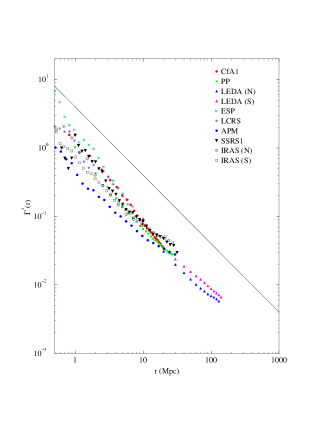
Fig. 1.–: The spatial density $\Gamma(r)$ computed in some VL samples of CfA1, PP, LEDA, APM, ESP, LCRS, SSRS1, IRAS and ESP and normalized to the corresponding factor, as explained in the text.

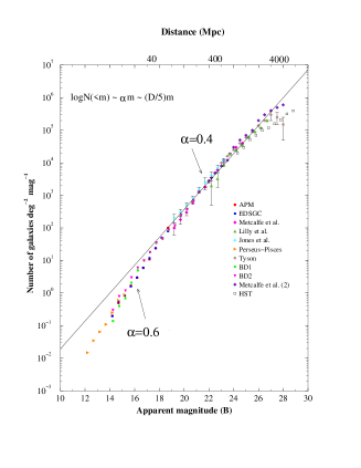
Fig. 2.–: Galaxy number counts as a function of the apparent magnitude ($m$) in the visible B-band. $\alpha=D/5\approx 0.6$

Fig. 3.–: Conditional density computed form one point in various VL samples of PP. The behavior of the average conditional density (Fig.2 Top panel) can be extended to larger scales by the conditional density form the vertex only for $r>\lambda$ where it becomes statistically meaningful. In the insert panel: Schematic behavior of the conditional density computed form a single point (the origin).

References

- [1] \Name Davis, M. \AndPeebles P. J. E. \ReviewAp.J. \Vol267 \Year1983 \Page465
- [2] \Name Coleman P.H. \AndPietronero L. \Review Phys.Rep. \Year1992 \Vol231, \Page311
- [3] \Name Binggeli B., Sandage A., Tammann G. A. \ReviewAstron. Astrophys. Ann. Rev.\Year1988\Vol 26\Page 509
- [4] \NameSylos Labini F. \AndPietronero L. \Review Astrophys.J. \Year1996 \Vol469 \Page 28
- [5] \NameSylos Labini F. et al \Review Physica A\Year1996 \Vol 230 \Page 368; \NameDi Nella H. et al \ReviewAstron.Astrophys.Lett. \Year1996 \Vol 308 \Page L33; \NamePietronero L. et al in \BookCritical Dialogues in Cosmology edited by \NameN. Turok (World Scientific) \Year1997
- [6] \NameStrauss M.A. et al \ReviewAp.J.\Year1990\Vol 361\Page 49; \NameFisher K. et al \Review MNRAS \Year1994 \Vol266\Page 50
- [7] \Name Guzzo L. et al \Review Ap.J.\Year1992 \Vol382\Page L9
- [8] \Name Peebles P.E.J. \BookPrinciples of physical cosmology (Princeton Univ.Press.)\Year1993
- [9] \NameSylos Labini F. \AndAmendola, L., \ReviewAstrophys.J. \Year1996 \Vol 468,\Page L1
- [10] \Name Sylos Labini F., Montuori M., Pietronero L. \ReviewPhysics Reports\Year1997 in Print
- [11] \Name Sylos Labini F. et al \Review Physica A \Year1996\Vol 266\Page 149
- [12] \Name Schechter P. \Review Ap.J. \Year1976 \Vol 203\Page 297
- [13] \Name Da Costa L. et al \Review Ap.J. \Year1994 \Vol 424 \PageL1