What Can Cosmic Microwave Background Observations
Already Say About Cosmological Parameters
in Open and Critical-Density Cold Dark Matter Models?

Abstract

We use a combination of the most recent cosmic microwave background (CMB) flat-band power measurements to place constraints on Hubble’s constant $h$ and the total density of the Universe $\Omega_{o}$ in the context of inflation-based cold dark matter (CDM) models with no cosmological constant. We use $\chi^{2}$ minimization to explore the 4-dimensional parameter space having as free parameters, $h$, $\Omega_{o}$, the power spectrum slope $n$ and the power spectrum normalization at $\ell=10$. Conditioning on $\Omega_{o}=1$ we obtain $h=0.33\pm 0.08$. Allowing $\Omega_{o}$ to be a free parameter reduces the ability of the CMB data to constrain $h$ and we obtain $0.26<h<0.97$ with a best-fit value at $h=0.40$. We obtain $\Omega_{o}=0.85$ and set a lower limit $\Omega_{o}>0.53$. A strong correlation between acceptable $h$ and $\Omega_{o}$ values leads to a new constraint $\Omega_{o}h^{1/2}=0.55\pm 0.10$. We quote $\Delta\chi^{2}=1$ contours as error bars, however because of nonlinearities of the models, these may be only crude approximations to $1\sigma$ confidence limits.

A favored open model with $\Omega_{o}=0.3$ and $h=0.70$ is more than $\sim 4\sigma$ from the CMB data best-fit model and is rejected by goodness-of-fit statistics at the $99\%$ CL. High baryonic models ($\Omega_{b}h^{2}\sim 0.026$) yield the best CMB $\chi^{2}$ fits and are more consistent with other cosmological constraints. The best-fit model has $n=0.91^{+0.29}_{-0.09}$ and $Q_{10}=18.0^{+1.2}_{-1.5}\;\mu$K. Conditioning on $n=1$ we obtain $h=0.55^{+0.13}_{-0.19}$, $\Omega_{o}=0.70$ with a lower limit $\Omega_{o}>0.58$ and $Q_{10}=18.0^{+1.4}_{-1.5}\>\mu$K. The amplitude and position of the dominant peak in the best-fit power spectrum are $A_{peak}=76^{+3}_{-7}\;\mu$K and $\ell_{peak}=260^{+30}_{-20}$.

Unlike the $\Omega_{o}=1$ case we considered previously, CMB $h$ results are now consistent with the higher values favored by local measurements of $h$ but only if $0.55\mbox{$\>\stackrel{{\scriptstyle<}}{{{}_{\sim}}}\>$}\Omega_{o}\mbox{$\>\stackrel{{\scriptstyle<}}{{{}_{\sim}}}\>$}0.85$. Using an approximate joint likelihood to combine our CMB constraint on $\Omega_{o}h^{1/2}$ with other cosmological constraints we obtain $h=0.58\pm 0.11$ and $\Omega_{o}=0.65^{+0.16}_{-0.15}$.

Subject headings: cosmic microwave background – cosmology: observations

1 INTRODUCTION

The ensemble of cosmological data prefers best-bet universes which seem to congregate in several distinct regions of parameter space (Ostriker & Steinhardt 1995, Viana 1996). Among the best-bet universes, open models figure prominently and are possibly the favorite candidate (Liddle et al. 1996a). This preference is mainly due to observational evidence (e.g., Willick et al. 1997, Carlberg et al. 1996, Dekel 1997). Further motivation for examining $\Omega_{o}<1$ models is that galaxy cluster baryonic fraction limits seem to be inconsistent with Big Bang nucleosynthesis (BBN) if $\Omega_{o}=1$ and $h\mathrel{\hbox{\hbox to0.0pt{\hbox{\lower 4.0pt\hbox{$\sim$}}\hss}\hbox{$>$}}}0.50$ ($h=H_{o}/100\;km\>s^{-1}Mpc^{-1}$). This “baryon catastrophe” has led some to believe that $\Omega_{o}<1$.

Recently, theoretical open universe models have been developed. Open-bubble inflation models have been developed by Ratra & Peebles (1994), Bucher, Goldhaber & Turok (1995), Yamamoto, Sasaki & Tanaka (1995). Open hybrid inflation has also been considered (García-Bellido & Linde 1997).

1.1 What Kind of Open Models We Consider and Why

CMB measurements have become sensitive enough to constrain cosmological parameters in restricted classes of models. In Lineweaver et al. (1997), (henceforth “paper 1”), we described our $\chi^{2}$ method and compared CMB data to predictions of COBE-normalized critical-density universes with Harrison-Zel’dovich ($n=1$) power spectra. We briefly looked at CDM and flat $\Lambda$ CDM models by exploring the $h-\Omega_{b}$ plane and the $h-\lambda_{o}$ plane. We used predominantly goodness-of-fit statistics to locate the regions of parameter space preferred by the CMB data.

In Lineweaver & Barbosa (1998), (henceforth “paper 2”), we used a similar technique, again in critical-density universes, to explore the 4-dimensional parameter space $h$, $\Omega_{b}$, $n$ and $Q$. We obtained the result that if $\Omega_{o}=1$ (and our other assumptions are correct) then the CMB data prefer surprisingly low values of the Hubble constant: $h\approx 0.30$. We found that four independent cosmological constraints also favored these low values in the $\Omega_{o}=1$ models considered. This is in contrast to local measurements of $h$ which seem to prefer $h\approx 0.65\pm 0.15$ (Freedman 1998, Tammann & Federspiel 1997).

The $\Omega_{o}=1$ assumption we have made in our previous analyses can be considered very restrictive since plausible values for $\Omega_{o}$ in the range $0.2\mbox{$\>\stackrel{{\scriptstyle<}}{{{}_{\sim}}}\>$}\Omega_{o}\mbox{$\>\stackrel{{\scriptstyle<}}{{{}_{\sim}}}\>$}1.0$ can change the power spectrum significantly. In this work we consider open models motivated by the question: Does our $h\approx 0.30$ result depend on the fact that we limited ourselves to $\Omega_{o}=1$? Would a favored open model ($h=0.7$ and $\Omega_{o}=0.3$) be acceptable to the combined CMB data? What pairs of $(h,\Omega_{o})$ values are compatible with the CMB data?

There are reasons to believe that $\Omega_{o}<1$ models will allow higher $h$ values. In paper 2 we found that the position of the primary acoustic peak in the angular power spectrum is a dominant feature determining the low value of $h$. The position of the peak is shifted towards higher $\ell$ values in $\Omega_{o}<1$ models and this should have the effect of increasing the $h$ values of the best-fit models. Motivated by this idea and the more general idea of increasing the size of the parameter space into interesting regions, in this paper we put constraints on the cosmological parameters $h$, $\Omega_{o}$, $n$, and the normalization at $\ell=10$ in the context of $\Omega_{o}\leq 1$ CDM models. We assume adiabatic initial conditions with no cosmological constant. As in paper 1 and 2, we take advantage of the recently available fast Boltzmann code to make the parameter-dependent model power spectra (Seljak and Zaldarriaga 1996). We do not consider $\Omega_{o}>1$ models because the code is not yet available.

The recent dynamic interplay between theory (providing a fast code to make model specific predictions) and observations (new measurements are coming in about once a month) is increasing our ability to distinguish models. Major efforts have been and are being put into obtaining flat-band power estimates. The synthesis of these efforts is an important step towards a more complete picture of the Universe. Since the main goal of two new CMB satellites (MAP and Planck Surveyor) is to constrain cosmological parameters, it is important and timely to keep track of the data’s increasing ability to reject larger regions of parameter space and put tighter constraints on preferred models. That is the purpose of this paper.

Previous analyses most closely related to this work include Ganga et al. (1996), White & Silk (1996), White et al. (1996), Hancock et al. (1998), Bond & Jaffe (1997), deBernardis et al. (1997). Although methods, models and data sets differ, in the limited cases where comparison is possible we have found no large discrepancies.

In Section 2 we summarize the method used to obtain the results and examine some of the special features of open models. In Section 3 we present our $h-\Omega_{o}$ results and in Section 4 we compare them to non-CMB results. In Section 5 we present our results for $n$, the normalization, $A_{peak}$ and $\ell_{peak}$. In Section 6 we discuss and summarize.

2 METHOD

2.1 Data and $\chi^{2}$ Analysis

We use a combination of the most recent CMB flat-band power measurements to place constraints on $h$, $\Omega_{o}$, $n$ and the normalization at $\ell=10$, $Q_{10}$ (see Section 2.2 for $Q_{10}$ definition). We examine how the constraints on any one of these parameters changes as we condition on as well as minimize with respect to the other parameters. We obtain best-fit values and approximate likelihood intervals for these parameters.

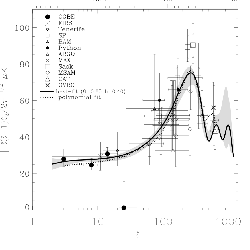
Fig. 1.—: Recent CMB observations compared with the best-fit model from Figure 4 The dotted line is a sixth order polynomial fit to the data which has a peak amplitude and position: $A_{peak}\approx 77\>\mu$K and $\ell_{peak}\approx 260$. The grey region represents the $\sim 1\sigma$ contour in Figure 4; that is, the power spectra from models within $\sim 1\sigma$ of the best-fit model are contained within the grey region. The small squares above and below the 5 Saskatoon points represent the $7\%$ correlated calibration uncertainty (Leitch 1998). The best-fit model has $n=0.91$, $Q_{10}=18.0\;\mu$K and $\Omega_{b}h^{2}=0.026$.

We update the data of paper 2 to include several more points:
$\bullet$ updated Tenerife point (Gutiérrez et al. 1997): $\delta T_{eff}=32.5^{+10.1}_{-8.5}\;\mu$K at $\ell_{eff}=20$
$\bullet$ new MSAM results (Cheng et al. 1997): $\delta T_{eff}=50^{+13}_{-9}\;\mu$K at $\ell_{eff}=159$ and $\delta T_{eff}=65^{+14}_{-10}\;\mu$K at $\ell_{eff}=263$
$\bullet$ new preliminary CAT results (Baker 1997): $\delta T_{eff}=47.3^{+9.3}_{-6.3}\;\mu$K at $\ell_{eff}=422$ and $\delta T_{eff}=43.2^{+13.5}_{-10.1}\;\mu$K at $\ell_{eff}=615$
$\bullet$ new preliminary OVRO result (Leitch 1998): $\delta T_{eff}=56^{+14}_{-11}\;\mu$K at $\ell_{eff}=537$.

The current CMB flat-band power estimates used in this analysis are listed in Table 1 and plotted in Figure 1. Since there is much scatter in the data, there is much scepticism about the ability of the points to prefer any particular region of parameter space. We showed in papers 1 and 2 however that a simple $\chi^{2}$ analysis of interesting restricted families of models is capable of showing substantial preferences for relatively small regions of parameter space. The scatter in the data is partially deceiving in the sense that averaging the data over broader bands in $\ell$ reduces the scatter and presents a surprisingly coherent power spectrum which roughly follows the polynomial fit in Figure 1.

Fig. 2.—: CMB power spectra showing the influence of $\Omega_{o}$, $\Omega_{b}h^{2}$ and $h$. These models are for $n=1$, $Q_{10}=17\>\mu$K. The dotted line represents the data. It is the same in all panels and is the same as in Figure 1. The peak amplitude $A_{peak}$ depends strongly on $h$ but also on $\Omega_{b}h^{2}$ and $\Omega_{o}$. The $\ell$ value of the peak, $\ell_{peak}$, is $\Omega_{o}$ dependent but also mildly $h$ dependent. In the lower right panel $\Omega_{o}=0.7$, $h=0.50$, $\Omega_{b}h^{2}=0.026$ fits the data quite well and is very close to the best-fit model for $n=1$ models (Figure 3).

Essentially, we are trying to find the parameters of the model that looks most like the dotted line in Figure 1. Figure 2 is an example of some of the model power spectra tested. For each point in the 4-D parameter space we obtain a value for $\chi^{2}(h,\Omega_{o},n,Q_{10})$. The parameter values at the minimum value ($\chi^{2}_{min}$) are the best-fit parameters. The error bars we quote for each parameter are from the maximum and minimum parameter values within the 4-D surface which satisfies $\chi^{2}(h,\Omega,n,Q_{10})=\chi^{2}_{min}+1$. To display the result we project this surface onto the two dimensions of our choice. The $\chi^{2}$ calculation is described in more detail in papers 1 and 2.

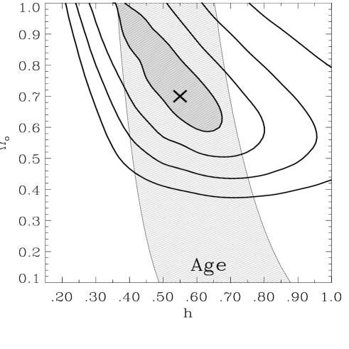
Fig. 3.—: Likelihood contours in the $h-\Omega_{o}$ plane. We condition on $n=1$ while $Q_{10}$ and $\Omega_{b}h^{2}$ are free to take on the value that minimizes the $\chi^{2}$ value at that point. The four contours correspond to $\chi^{2}_{min}+\Delta\chi^{2}$ where $\Delta\chi^{2}=[1,4,9,16]$ (See Section 2.1). The best-fit parameters are $h=0.55^{+0.13}_{-0.19}$ and $\Omega_{o}=0.70$ with $\Omega_{o}>0.58\;(\sim 1\sigma$). The lightly shaded region represents the age constraint $10<t_{o}<18$ Gyr.

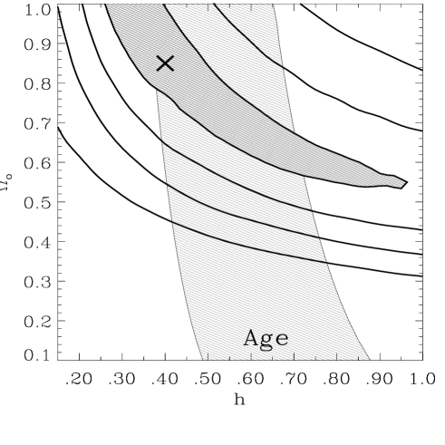
Fig. 4.—: Same as previous figure except here we no longer condition on $n=1$. Recall that our error bars are obtained from the projection of the $\Delta\chi^{2}=1$ contour onto an axis. Thus at $\sim 1\sigma$, $h$ is free to take on any value between $0.26$ and $0.97$. At the minimum, $h=0.40^{+0.57}_{-0.14}$ and $\Omega_{o}=0.85$ with $\Omega_{o}>0.53$. The elongated $\Delta\chi^{2}=1$ contour means that $h$ and $\Omega_{o}$ are highly correlated. This correlation leads to a new constraint: $0.45<\Omega_{o}h^{1/2}<0.65$ which should be compared to the constraint on the same quantity from cluster baryonic fractions (see Figure 5 and Section 4.1).

Figure 3 is the first in a series of contour plots which illustrates our results. The four contours correspond to $\chi^{2}_{min}+\Delta\chi^{2}$ surfaces where $\Delta\chi^{2}=[1,4,9,16]$. The interpretation of these contours is not straightforward. The conditions under which these contours can be projected onto an axis yielding $1,\;2,\;3\;$ and $4\sigma$ confidence intervals is described in Press et al. (1992 p 690) (see also Avni 1976). These conditions are: i) the errors are normally distributed and ii) the model is linear in the parameters or that a linear approximation reasonably represents the models within the range of parameters of interest. deBernardis et al. (1997) find that the error bars are approximately normal.

Although the model power spectra are nonlinear in the parameters, an approximation linear in the parameters may be able to represent the power spectrum near the $\chi^{2}$ minima. For example, in Figure 2, several families of models are plotted. The data have a maximum $\ell_{eff}$ value of $615$. The ability of the $\chi^{2}$ to discriminate between models comes almost exclusively from the data in the range $2\mbox{$\>\stackrel{{\scriptstyle<}}{{{}_{\sim}}}\>$}\ell_{eff}\mbox{$\>\stackrel{{\scriptstyle<}}{{{}_{\sim}}}\>$}430$. The strongest nonlinearities in the models (typified by regions where the models do not trace each other but overlap in complicated ways) are in the $\ell$ range to which the data is not sensitive. It could be argued that the relevant parts of the models may be approximated by the first two terms of a Taylor expansion of the power spectrum around the best-fit parameter values. The accuracy of this linear approximation is a measure of the accuracy of the correspondence we would like to establish between the $\chi^{2}_{min}+1$ contour and the $1\sigma$ confidence interval. The ellipticities of the contours in Figures 3, 4 and 7 are also a measure of the accuracy of the linear approximation; exactly linear models would give concentric, exact ellipses with identical orientations and position angles and with semimajor axes in the ratios 1:2:3:4. We conclude that the error bars that we derive from the $\chi^{2}_{min}+1$ contours may be useful approximations to $1\sigma$ confidence limits, but that the $\chi^{2}_{min}+4$, 9, and 16 contours are at best rough guides to the 2, 3, and 4 $\sigma$ confidence intervals. Work is in progress to quantify the accuracy of the linear approximation. Bond, Jaffe & Knox (1998) have done a preliminary analysis comparing a $\chi^{2}$-minimization analysis of flat-band estimates to a more complete pixel-based treatment. Their general conclusion is that our “radical data compression method works…sort of” since the minima found by the two techniques agree fairly well.

2.2 Normalization and Definition of $Q_{10}$

We normalize in the middle of the COBE DMR data ($\ell=10$) rather than at the edge ($\ell=2$) to reduce the otherwise strong correlation between the best-fit slope and normalization. We parametrize the normalization at $\ell=10$ using the symbol $Q_{10}$ defined by

$$10(10+1)C_{10}=\frac{24\pi}{5}\frac{Q_{10}^{2}}{T_{o}^{2}}.$$ (1)

Equation 1 is simply a way to write $C_{10}$ with the added convenience that for an $n=1$ pure Sachs-Wolfe spectrum ($C_{\ell}\propto 1/(\ell(\ell+1))$), $Q_{10}$ is equivalent to the power spectrum normalizing quadrupole $Q_{rms-PS}$ (see Smoot et al. 1992).

2.3 Saskatoon Calibration

We have used the new calibration (Leitch 1998) for the Saskatoon results whereby the nominal Saskatoon calibration (Netterfield et al. 1995, Netterfield et al. 1997) is increased by $5\%$ with a correlated calibration uncertainty around this new value of $7\%$. We treat the calibration of the 5 Saskatoon points as a nuisance parameter “$u_{sk}$” coming from a Gaussian distribution with a dispersion of $7\%$ (rather than the $14\%$ used in paper 2). In this sense our error bars include an estimate of the Saskatoon calibration uncertainty.

In general the minimum $\chi^{2}$ fits prefer $u_{sk}\approx 0.86$. This can be understood quite easily by examining Figure 1. The little boxes above and below the Saskatoon points are $\pm 7\%$ of the central values. $u_{sk}=0.86$ corresponds to $-14\%$. Moving all 5 Saskatoon points down by $\sim 14\%$ gives the best agreement with the dotted line, representing all the data. Thus $u_{sk}\approx 0.86$ is the preferred value.

There are 32 data points and in the most general case where all 5 parameters ($h$, $\Omega_{o}$, $n$, $Q_{10}$, $u_{sk}$) are free, there are 27 degrees of freedom (= 32 - 5). When both $h$ and $\Omega_{o}$ are low and thus nominally $\Omega_{o}<\Omega_{b}$; we set $\Omega_{b}=\Omega_{o}$, thus creating purely baryonic models in the lower left corners of Figures 3 and 4. Computer limits restrict the number of discrete $\Omega_{b}h^{2}$ values we can test. We have performed all calculations for each of 3 values of $\Omega_{b}h^{2}$: $\Omega_{b}h^{2}\in\{0.010,0.015,0.026\}$. Thus we have explored three 4-D slices of parameter space. For completeness we have also minimized with respect to $\Omega_{b}h^{2}$ in the same way we have for the other parameters, but the $\Omega_{b}h^{2}$ minimization is restricted to only three discrete values. The results from this highly discretized BBN range minimization are indicated by “$\;*\;$” in the $\Omega_{b}h^{2}$ column of Table 2.

2.4 Physical Effects in Open Models

Acoustic oscillations of the baryon–photon fluid at recombination produce peaks in the CMB power spectrum around degree angular scales. It is convenient to discuss power spectra in terms of the amplitude and the position of the first such peak: $A_{peak}$ and $\ell_{peak}$. For example, the amplitude and position of the polynomial fit to the data (dotted line in Figure 1) are $A_{peak}=77\;\mu$K and $\ell_{peak}=260$. For the physics of the acoustic peaks, see the pioneering work by Hu (1995) and Hu & Sugiyama (1995a, 1995b).

In Figure 2 we plot CMB power spectra to display the influence of $\Omega_{o}$ and $h$ and $\Omega_{b}h^{2}$. The dotted line is the same in each panel, is the same as in Figure 1 and represents the data. These models are for $n=1$, $Q_{10}=17\>\mu$K. In Figure 2 we can see that the peak amplitudes $A_{peak}$ depend strongly on $h$ and $\Omega_{b}h^{2}$. Higher values of $\Omega_{b}h^{2}$ lead to larger Doppler peaks due to the enhanced compression caused by a larger effective mass (more baryons per photon) of the oscillating fluid. For a given $\Omega_{b}h^{2}$, a small $h$ means high $A_{peak}$. $Q_{10}$ variations would raise and lower the entire curve while variations in the slope $n$ would raise and lower $A_{peak}$.

In Figure 2, when $h\downarrow$, $\ell_{peak}\uparrow$. Similarly, as $\Omega_{o}\downarrow$, $\ell_{peak}\uparrow$. The $\Omega_{o}$ dependence of $\ell_{peak}$ is a purely geometric effect. The more open the universe, the smaller the angle subtended by the same physical size. The main point of Figure 2 is that lowering $h$ and lowering $\Omega_{o}$ both have the same effect of raising $\ell_{peak}$. In paper 1 and 2 we maintained that it was predominantly the position of the peak that favored low $h$ in $\Omega_{o}=1$ models. Here we see that lowering $\Omega_{o}$ can raise $\ell_{peak}$ to fit the data, hence $h$ does not have to be as low. The behaviour of $A_{peak}$ and $\ell_{peak}$ can be tabulated as,

$A_{peak}\uparrow$	$h\downarrow$	$\Omega_{o}\downarrow$ (for $\Omega_{o}\mbox{$\>\stackrel{{\scriptstyle>}}{{{}_{\sim}}}\>$}0.6$)	$\Omega_{b}h^{2}\uparrow$	$n\uparrow$
$\ell_{peak}\uparrow$	$h\downarrow$	$\Omega_{o}\downarrow$

which is to be read “$A_{peak}$ goes up when $h$ or $\Omega_{o}$ go down or when $\Omega_{b}h^{2}$ or $n$ go up”. See Hu, Sugiyama & Silk (1997) for more details.

3 RESULTS FROM THE $h-\Omega_{o}$ DIAGRAM

The $h-\Omega_{o}$ diagram is a convenient framework in which to explore and present a combination of cosmological parameters. The regions preferred by the CMB are shown in Figures 3 and 4. The results from these figures are given in the first two sections of Table 2 which also contains the main results of this paper for $h$, $\Omega_{o}$, $n$ and $Q_{10}$. For each result, the conditions under which it was obtained are listed and these conditions are relaxed as we move from the top to the bottom. Table 2 also lists $\chi^{2}$ values and the corresponding probabilities $P(\chi^{2}<)$ of obtaining $\chi^{2}$ values smaller than the values actually obtained, under the assumption that the errors on the data points are Gaussian. $\chi^{2}$ values and probabilities are discussed in Section 5.3.

3.1 $h$ Results

For $\Omega_{o}=1$ we get $h=0.33\pm 0.08$, which is the same low $h$ value we obtained in paper 2. The new Saskatoon calibration and the new data used here do not change our previous result.

In Figure 3 we present the likelihood contours in the $h-\Omega_{o}$ plane for $n=1$. The minimum is at $h=0.55^{+0.13}_{-0.19}$. The minimum $\chi^{2}$ value and the probability of obtaining a smaller value for that model are $\chi^{2}_{min}=21.4$ and $P(\chi^{2}<)=23.4\%$ respectively. Thus the fit is “good”.

Figure 4 is the same as Figure 3 except we no longer condition on $n=1$. The best-fit $h$ value stays low but higher and lower $h$ values are now acceptable at $\sim 1\sigma$. Thus, uncertainty in $n$ plays an important role in the inability of CMB data to determine $h$. The banana-shaped $\Delta\chi^{2}=1$ contour can be projected onto an axis to yield an approximation to a $1\sigma$ confidence interval around the best-fit value. Thus, $0.26<h<0.97$ or $h=0.40^{+0.57}_{-0.14}$.

A favored open model with $\Omega_{o}=0.3$ and $h=0.70$ is more than $\sim 4\sigma$ from the CMB data best-fit model and can be rejected based on goodness of fit at the 99% confidence level. In contrast to our previous $\Omega_{o}=1$ results, allowing $\Omega_{o}<1$ permits much larger $h$ values and there is no longer a disagreement with more direct local measurements of $h$.

3.2 $\Omega_{o}$ Results

Our $\Omega_{o}$ results are also given in Table 2. In Figure 3 ($n=1$) we obtain $\Omega_{o}=0.70$ and set a lower limit $\Omega_{o}>0.58$. We obtain no upper limit because we were unable to test $\Omega_{o}>1$ models. In Figure 4 we obtain $\Omega_{o}=0.85$ with a lower limit of $\Omega_{o}>0.53$ at $\sim 1\sigma$ and $\Omega_{o}>0.43$ at $\sim 2\sigma$. Thus the CMB can place important constraints on these models.

If we assume that $h\approx 0.65\pm 0.15$ (as indicated by local $h$ measurements) then the CMB data prefer a density in the range $0.54\mbox{$\>\stackrel{{\scriptstyle<}}{{{}_{\sim}}}\>$}\Omega_{o}\mbox{$\>\stackrel{{\scriptstyle<}}{{{}_{\sim}}}\>$}0.84$ and a power spectral slope $0.96\mbox{$\>\stackrel{{\scriptstyle<}}{{{}_{\sim}}}\>$}n\mbox{$\>\stackrel{{\scriptstyle<}}{{{}_{\sim}}}\>$}1.12$.

3.3 A New Constraint on $\Omega_{o}h^{1/2}$

The variations in $n$ and $\Omega_{b}h^{2}$ permit the large range of $h$ seen in Figure 4. For example, for the highest values of $h$, $n\approx 1.18$ and $\Omega_{b}h^{2}=0.026$ while for the lowest $h$ values $n\approx 0.85$ and $\Omega_{b}h^{2}=0.010$. $n$ variations alone are not sufficient to permit very high $h$ values. For example if we let $n$ be free but we condition on $\Omega_{b}h^{2}=0.010$ then $h$ remains small: $h<0.42$. If we condition on $\Omega_{b}h^{2}=0.015$ then $h<0.51$. $n$ and $\Omega_{b}h^{2}$ are keeping the peak amplitude fit correctly. High $h$ values suppress the peak height but this is compensated for by high $n$ and $\Omega_{b}h^{2}$.

The elongated banana-shaped $\Delta\chi^{2}=1$ contour in Figure 4 means that $h$ and $\Omega_{o}$ are anti-correlated. In Figure 2 we see that $\ell_{peak}\uparrow$ when $h\downarrow$ or $\Omega_{o}\downarrow$. Thus high $\Omega_{o}$ go with low $h$ and low $\Omega_{o}$ go with high $h$. The $\Delta\chi^{2}=1$ contour in Figure 4 traces out this strong anti-correlation. To get a constraint on two parameters simultaneously we need to look at the $\Delta\chi^{2}=2.3$ contour. This can be described by $\Omega_{o}h^{1/2}=0.55\pm 0.10$. This should be compared to the constraint on the same quantity from cluster baryonic fractions (see Figure 5 and Section 4.1).

4 NON-CMB CONSTRAINTS IN THE $h-\Omega_{o}$ PLANE

To view our results within a larger picture, we compare them to other cosmological measurements and identify what the CMB constraints can add to this picture. The independent non-CMB cosmological measurements are summarized below. They are the same constraints used in paper 2 (with modifications described below) and we now include local measurements of $h$.

Peacock & Dodds (1994) made an empirical fit to the matter power spectrum using a shape parameter $\Gamma$. For $\Omega_{o}\leq 1$ models, $\Gamma$ can be written as (Sugiyama 1995)

$$\Gamma=h\>\Omega_{o}\>exp\left[-\Omega_{b}\left(\frac{\Omega_{o}+1}{\Omega_{o}}\right)\right].$$ (2)

We adopt the $2\sigma$ limits of the empirical fit of Peacock & Dodds (1994)(see also Liddle et al. 1996a) and include the $n$ dependence,

$$0.222<\Gamma-0.32\left(\frac{1}{n}-1\right)<0.293.$$ (3)

with the assumption that $0.8\leq n\leq 1.2$.

4.1 X-ray Cluster Baryonic Mass Fraction

Assuming that clusters are a fair sample of the Universe, observations of the X-ray luminosity and the angular size of galaxy clusters can be combined to constrain the quantity $\frac{\Omega_{b}}{\Omega_{o}}h^{3/2}$. We adopt the range $0.04<\frac{\Omega_{b}}{\Omega_{o}}h^{3/2}<0.10$ (White et al. 1993) with a central value of $0.06$ (Evrard 1997). We include the uncertainty in the value of $\Omega_{b}$ by replacing $\Omega_{b}$ with the BBN range $[0.010\>h^{-2},0.026\>h^{-2}]$ yielding the limits $0.10<\Omega_{o}\>h^{1/2}<0.65$, and the central value $\Omega_{o}\>h^{1/2}=0.25$.

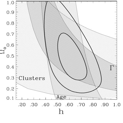
Fig. 5.—: This plot has no CMB information in it. The three bands are constraints from three non-CMB cosmological measurements discussed in Section 4. The “Age” of the oldest stars in globular clusters: $10<t_{o}<18$ Gyr, the baryonic fraction in “Clusters” of galaxies: $0.10<\Omega_{o}h^{1/2}<0.65$ and the matter power spectrum shape parameter “$\Gamma$”: $0.169<\Gamma<0.373$. The thick contours are approximate $1\sigma$ and $2\sigma$ regions from a joint likelihood of these three constraints with the added constraint from local measurements that $h=0.65\pm 0.15$. The results: $h=0.60^{+0.15}_{-0.10}$ and $\Omega_{o}=0.45^{+0.26}_{-0.17}$. An uncertainty of the baryonic fraction $0.010<\Omega_{b}h^{2}<0.026$ has been included in the constraints. In flat models the three constraints shown favor low values of $h\sim 0.40$ incompatible with local measurements of $h$. In the open models considered here, this disagreement disappears.

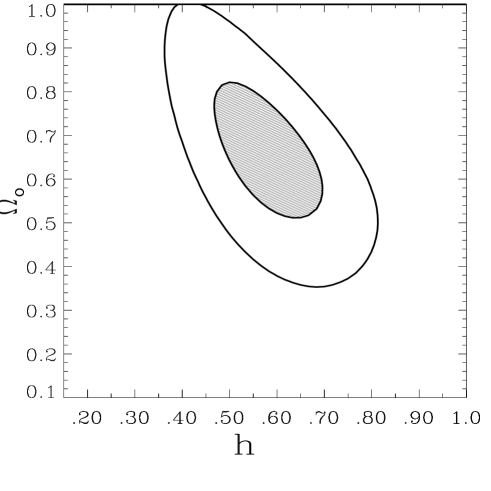
Fig. 6.—: Approximate $1\sigma$ and $2\sigma$ contours from a joint likelihood of the new CMB constraint $\Omega_{o}h^{1/2}=0.55\pm 0.10$ with the four constraints shown in Figure 5. The results: $h=0.58\pm 0.11$ and $\Omega_{o}=0.66^{+0.16}_{-0.15}$. Popular $\Omega_{o}=1$ and $(\Omega_{o}=0.3,h=0.70)$ models are $\approx 2\sigma$ from the best fit.

4.2 Limits on the Age of the Universe from the Oldest Stars in Globular Clusters

Although the determinations of the age of the oldest stars in globular clusters are $h$- and $\Omega_{o}$-independent, they do depend on the distance assigned to the globular clusters of our Galaxy. In paper 2 we used $11<t_{o}<18$ Gyr with a central value of 14 Gyr. We now adopt $10<t_{o}<18$ Gyr with a central value of 13 Gyr because the recent Hipparcos recalibration of the local distance ladder increases the distance to the globular clusters (Feast & Catchpole 1997, Gratton et al. 1997, Reid 1997). This lowers the inferred ages by about $\sim 5-10\%$ depending on what values were used in the calculation of the globular cluster distances.

Age determinations are $\Omega_{o}$ and $\lambda_{o}$ independent but converting them to limits on Hubble’s parameter depends on $\Omega_{o}$ and on our $\lambda_{o}=0$ assumption. For a flat Universe with $\lambda_{o}=0$ and $t_{o}$ expressed in Gyr, $h=(6.52/t_{o})$. In an open universe

$$h=\left(\frac{9.78}{t_{o}}\right)\!\left[\frac{1}{1-\Omega_{o}}-\frac{\Omega_{o}}{2(1-\Omega_{o})^{3/2}}\cosh^{-1}\!\left(\frac{2-\Omega_{o}}{\Omega_{o}}\right)\right],$$ (4)

where the term in square brackets is 2/3 for $\Omega_{o}=1$ and goes to 1 as $\Omega_{o}\rightarrow 0$. The constraint $10<t_{o}<18$ Gyr, inserted into Equation 4, provides the “Age” constraint on $h$ used in Figures 3, 4 and 5.

4.3 Summary of Constraints Used

The constraints we adopt from cluster baryonic fraction, the ages of the oldest stars in globular clusters, the matter density power spectrum shape parameter $\Gamma$ and local measurements of $h$ are,

Clusters	$0.10$	$<$	$\Omega_{o}\;h^{1/2}$	$<$	$0.65$
Age [Gyr]	$10$	$<$	$t_{o}$	$<$	$18$
$\Gamma$	$0.169$	$<$	$\Gamma$	$<$	$0.373$
Hubble	$0.50$	$<$	$h$	$<$	$0.80$

where the respective central values adopted are $\Omega_{o}\;h^{1/2}=0.25$, $t_{o}=13$ Gyr, $\Gamma=0.25$ and $h=0.65$.

The first three constraints are illustrated by the three bands in Figure 5. The $1\sigma$ and $2\sigma$ regions from an approximate joint likelihood of all four constraints are also shown (see paper 2, Section 4.5 for details). The $1\sigma$ region yields: $h=0.60^{+0.15}_{-0.10}$ and $\Omega_{o}=0.45^{+0.26}_{-0.17}$. If we consider only the first three constraints the result is $h=0.60^{+0.18}_{-0.21}$ and $\Omega_{o}=0.45^{+0.43}_{-0.17}$. Thus, in $\Omega_{o}\leq 1$ models, there is good agreement between the first three constraints and local measurements of $h$. This was not the case for the $\Omega_{o}=1$ universes tested in paper 2 where the first three constraints favored lower values; $h\approx 0.40$ (notice in Figure 5 that for $\Omega_{o}=1$, $h\approx 0.40$ is preferred).

An uncertainty of the baryonic fraction of $0.010<\Omega_{b}h^{2}<0.026$ has been included in both the cluster and $\Gamma$ constraints. We have also made a figure analogous to Figure 5 but with a smaller BBN uncertainty around a higher value, $0.022<\Omega_{b}h^{2}<0.026$. For this case, the lower limits of the “Cluster” and “$\Gamma$” bands are raised, thus narrowing the $1\sigma$ region.

4.4 Comparison of CMB and Non-CMB Constraints in the $h-\Omega_{o}$ Plane

What does the CMB add to the larger picture provided by these non-CMB measurements?

$\bullet$ Overall consistency: A superposition of Figures 4 and 5 shows that the $\sim 1\sigma$ regions of CMB and non-CMB overlap for $0.52\mbox{$\>\stackrel{{\scriptstyle<}}{{{}_{\sim}}}\>$}h\mbox{$\>\stackrel{{\scriptstyle<}}{{{}_{\sim}}}\>$}0.67$ and $0.58\mbox{$\>\stackrel{{\scriptstyle<}}{{{}_{\sim}}}\>$}\Omega_{o}\mbox{$\>\stackrel{{\scriptstyle<}}{{{}_{\sim}}}\>$}0.71$.

$\bullet$ More detailed consistency: The region of overlap of the first three constraints and the CMB is in agreement with local measurements of $h$. This agreement between CMB, three independent cosmological measurements and local $h$ measurements is non-trivial; in paper 2, although we had agreement between the CMB and three independent cosmological measurements, the agreement was at $h\sim 0.35$ and did not agree with local $h$ measurements.

$\bullet$ New constraint: We find a tight new model-dependent constraint $\Omega_{o}h^{1/2}=0.55\pm 0.10$ which favors the higher values of the cluster constraint on this same quantity.

$\bullet$ Preference for high $\Omega_{b}h^{2}$: Inside the $\Delta\chi^{2}=1$ contour (except for a small region to the left of the best fit) of Figure 4, the $\chi^{2}_{min}$ is for $\Omega_{b}h^{2}=0.026$. The consistency between the non-CMB constraints and the CMB constraints is stronger for higher values of $\Omega_{b}h^{2}$. This improved consistency and slightly better fit indicates that high $\Omega_{b}h^{2}$ is preferred, lending some support to Tytler et al. (1997) values.

$\bullet$ New argument for $n\sim 1$: Figure 3, where $n=1$, has a minimum inside the joint likelihood $1\sigma$ contour of Figure 5. In this sense it is more consistent with the combined constraints of Figure 5 than are the results of Figure 4. We can turn the argument around and say that the non-CMB constraints favor $n\sim 1$ based on this consistency.

$\bullet$ More precise combined constraint: Combining the CMB constraint on $\Omega_{o}h^{1/2}$ with the non-CMB contours in Figure 5 we obtain: $h=0.58\pm 0.11$ and $\Omega_{o}=0.66^{+0.16}_{-0.15}$ (see Figure 6).

$\bullet$ Rejection of a favored model: The $\Omega_{o}=0.3$, $h=0.70$ model is acceptable to the non-CMB measurements but is more than $\sim 4\sigma$ away from the best-fit CMB model in Figure 4 and can be rejected based on goodness of fit at the $99\%$ CL.

Liddle et al. (1996a) have examined open models with $\lambda_{o}=0$. They consider the shape parameter $\Gamma$, bulk flows, the abundance of clusters and the abundance of Ly-$\alpha$ systems and the age of the Universe. They find a good fit for $\Omega_{o}>0.35$ and an alarmingly low $h$ value for $\Omega_{o}\sim 1$. Assuming $h>0.6$ (as indicated by many recent measurements) they get $0.30<\Omega_{o}<0.60$. If we assume $h>0.6$ we obtain $0.53<\Omega_{o}<0.75$ from the CMB analysis, and $0.3<\Omega_{o}<0.70$ from the first three non-CMB constraints. Thus we find consistent but slightly higher allowed intervals for $\Omega_{o}$.

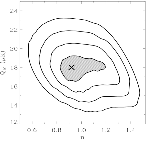
Fig. 7.—: Likelihood contours in the $n-Q_{10}$ plane with $h$ and $\Omega_{o}$ as free parameters. The minimum is $n=0.91^{+0.29}_{-0.09}$, $Q_{10}=18.0^{+1.2}_{-1.5}\;\mu$K. Notice that there is no strong correlation between $n$ and $Q_{10}$ as there is between $n$ and $Q_{rms-PS}$ (e.g. Lineweaver 1994).

5 RESULTS FOR $n$, $Q_{10}$, $A_{peak}$ AND $\ell_{peak}$

5.1 Results for $n$ and $Q_{10}$

Our $n$ results are listed in Table 2. Conditioning on $\Omega_{o}=1$ we get $n=0.91^{+0.10}_{-0.10}$. Figure 7 displays our most general result in the $n-Q_{10}$ plane and yields $n=0.91^{+0.29}_{-0.09}$. Thus the minimum is unchanged and the error bars increase slightly in this more general case. The best-fit value of $n$ is a robust result in the sense that it does not change from the $\Omega_{o}=1$ to the $\Omega_{o}\leq 1$ case.

For $\Omega_{o}=1$ and $n=1$ we get $Q_{10}=17.0^{+1.4}_{-1.0}\;\mu$K. For $\Omega_{o}$ free and $n=1$ we obtain $Q_{10}=18.0^{+1.4}_{-1.5}\;\mu$K. Conditioning on $\Omega_{o}=1$ we obtain $Q_{10}=17.5^{+1.1}_{-1.1}\;\mu$K. And finally with all other parameters free we get $Q_{10}=18.0^{+1.2}_{-1.5}\;\mu$K (Figure 7). We can also express this normalization in terms of $C_{10}$,

$$10^{11}C_{10}=0.597\left(\frac{Q_{10}}{18.0\;\mu K}\right)^{2}.$$ (5)

This normalization at the best-fit values for $h$, $\Omega_{o}$, $n$ and $\Omega_{b}h^{2}$ should be compared to the slightly higher, more general (but COBE DMR only) Bunn & White (1997) normalization which is a function of the first and second derivatives of the power spectrum at $\ell=10$.

5.2 Results for $A_{peak}$ and $\ell_{peak}$

We can get a rough idea of the values of $A_{peak}$ and $\ell_{peak}$ preferred by the data from the sixth order polynomial fit shown in Figure 1. This yields $A_{peak}\approx 77\;\mu$K and $\ell_{peak}\approx 260$. We can also make a more careful model-dependent estimate of $A_{peak}$ and $\ell_{peak}$ by looking at the power spectrum of the best-fit model in Figure 4 and by examining the power spectra from models along the edge of the $\Delta\chi^{2}=1$ contour. The power spectrum of the best-fit model gives us central values for $A_{peak}$ and $\ell_{peak}$ while the power spectra of the models along the edge of the $\Delta\chi^{2}=1$ contour yield error bars on these central values. The result is $A_{peak}=76^{+3}_{-7}\;\mu$K and $\ell_{peak}=260^{+30}_{-20}$. It should be remembered that these results depend on the correctness of the family of models we are considering ($\Omega_{o}\leq 1$, $\lambda_{o}=0$).

5.3 $\chi^{2}$ and Probabilities P$(\chi^{2}<)$

The minimum $\chi^{2}$ values are given in Table 2 along with the probability of obtaining smaller values under a Gaussian assumption for the errors on the flat-band power estimates. The range of minimum-$\chi^{2}$ values and their corresponding probabilities are $[20.9<\chi^{2}<24.6]$ and $[18.2<P<35.2]$. These $\chi^{2}$ values are “good” and border on “too good”. The highest $\chi^{2}$ values and the highest probabilities are when we condition on $h=0.50$ with $\Omega_{o}=1$ giving substantially worse fits than $h$ free. The lowest probabilities are when we condition on $\Omega_{o}=1$ and $\Omega_{b}h^{2}=0.026$.

We have added the calibration uncertainty in quadrature to the statistical error bars on the flat-band power estimates. If we were more conservative we would add them linearly. In this case the $\chi^{2}$ values would be even lower and the fits even better, i.e., “too good”.

Figure 2 shows how the CMB power spectra vary as a function of $\Omega_{b}h^{2}$. In Table 2 we have included results for each value of $\Omega_{b}h^{2}$ separately. The $\Omega_{b}h^{2}=0.010$ minima have the highest $\chi^{2}$ values while the $\Omega_{b}h^{2}=0.026$ minima have the lowest and are thus identical to the $\chi^{2}$ of the restricted minimization with respect to $\Omega_{b}h^{2}$ (see Section 2.3).

$\Omega_{o}=1$ models are a subset of the models examined here. The differences between the $\Omega_{o}=1$ results reported here and those reported in paper 2 are small and can be understood by the three differences in the analysis. In the present work i) we only look at three discrete values of of $\Omega_{b}h^{2}$ (in paper 2 we explored the $h-\Omega_{b}$ plane), ii) we include 5 more data points, iii) we use a Saskatoon calibration $5\%$ higher with a smaller uncertainty.

6 DISCUSSION AND SUMMARY

6.1 Review of Results

We use CMB flat-band power estimates to obtain constraints on $h$, $\Omega_{o}$, $n$ and $Q_{10}$ in the context of $\Omega_{o}\leq 1$ CDM models of the Universe. Conditioning on $\Omega_{o}=1$ we obtain $h=0.33\pm 0.08$. Allowing $\Omega_{o}$ to be a free parameter reduces the ability of the CMB data to constrain $h$ and we obtain $0.26<h<0.97$ with the minimum at $h=0.40$. We obtain $\Omega_{o}=0.85$ and set a lower limit $\Omega_{o}>0.53$. We find a strong correlation between acceptable $h$ and $\Omega_{o}$ values leading to the new CMB constraint $\Omega_{o}h^{1/2}=0.55\pm 0.10$. We also obtain $n=0.91^{+0.29}_{-0.09}$ and $Q_{10}=18.0^{+1.2}_{-1.5}\;\mu$K. High baryonic models ($\Omega_{b}h^{2}\sim 0.026$) yield the best CMB $\chi^{2}$ fits which also are more consistent with other cosmological constraints. We find that a favored open model with $\Omega_{o}=0.3$ and $h=0.70$ is more than $\sim 4\sigma$ from the CMB data best-fit model and can be rejected at the 99% CL based on goodness of fit.

6.2 Consistency with Non-CMB Measurements

In the flat CDM models of paper 2 we found that $h\sim 0.30$. This value was consistent with four non-CMB constraints but in disagreement with local measurements of $h$. Considering $\Omega_{o}\leq 1$ models for $\Omega_{b}h^{2}$ fixed at $0.015$ we again find $h$ limited to values $\mbox{$\>\stackrel{{\scriptstyle<}}{{{}_{\sim}}}\>$}0.50$ and best-fit values of $\Omega_{o}$ near 1. It is not until we allow $\Omega_{b}h^{2}=0.026$ that a much larger interval of $h$ is allowed at the $\sim 1\sigma$ level. For this most general case, the results from the CMB, the same non-CMB constraints as used previously and local measurements of $h$ are all consistent with $h\approx 0.58$ and $\Omega_{o}\approx 0.66$.

The $\sigma_{8}$ that corresponds to our best-fit model is $\sigma_{8}=0.51^{+1.76}_{-0.20}$. This is consistent with results from independent measurements which favor the interval $[0.4,0.9]$ (Viana & Liddle 1996, Eke et al. 1996). Our $\Omega_{o}$ results are also broadly consistent with bulk flow measurements which yield roughly $\Omega_{o}>0.4$ (Dekel 1997).

CMB constraints are independent of other cosmological measurements and are thus particularly important. The fact that reasonable $\chi^{2}$ values are obtained means that the current CMB data are consistent with inflation-based $\Omega_{o}\leq 1$ CDM models for a broad range of $h$ values. In the context of the models considered, the CMB results are consistent with three other independent cosmological measurements and are now also in agreement with local measurements of $h$. This consistency was not present in $\Omega_{o}=1$ models.

6.3 Review of Assumptions

The results we have presented here are valid under the assumption of inflation-based CDM models with Gaussian adiabatic initial conditions and with no cosmological constant. We have not considered early reionization scenarios or hot dark matter. We have also not included any gravitational wave contributions which seem to make the fits slightly worse without changing the location of the best-fit parameters (Liddle et al. 1996b, Bond and Jaffe 1997). With only scalar perturbations, deviations of the power spectrum from power-law behavior is negligible in open models (Garcia-Bellido 1997). Supercurvature modes are not included in the power spectra models (Seljak & Zaldarriaga 1996) because they are in general important only for $\ell\mbox{$\>\stackrel{{\scriptstyle<}}{{{}_{\sim}}}\>$}5$ and thus difficult to measure because of cosmic variance.

It is possible that one or more of our basic assumptions is wrong, or we could simply be looking at too restricted a region of parameter space. Topological defects may be the origin of structure. Using the same data and $\chi^{2}$-minimization analysis, we find (Durrer et al. 1997) that several classes of scalar-component-only global topological defect models also produce acceptable fits to the data although the goodness of fit of these models is not as good as the models we consider here. In other words, goodness-of-fit statistics from current CMB data have a slight preference for the inflation-based models we have considered over the topological defect models we have considered.

6.4 Future Improvements

In addition to the $h$, $\Omega_{o}$, $n$, $Q_{10}$ and $\Omega_{b}h^{2}$ considered here, regions of a larger dimensional parameter space deserve further investigation including $\lambda_{o}$, $\Omega_{HDM}$, $\Omega_{b}$, early reionization parameters such as $z_{reion}$, tensor mode parameters $n_{T}$ and $T$, the inflaton potential $r$, iso-curvature or adiabatic initial conditions and topological defect models with their additional parameters.

The fact that we obtain acceptable $\chi^{2}$ values in our 4-D parameter space lends some support to the idea that we may be close to the right model. If the Universe is not well described by these models then as the data improve, work like this will show poor $\chi^{2}$ fits and other regions of parameter space will be preferred.

To increase the parameter-constraining power of the measurements, observations need to be made in regions of $\ell$-space that have no or few measurements. In Figure 1 we can identify these regions: $600<\ell<1200$, $20<\ell<50$ and $180<\ell<400$. More than a dozen on-going small-angular-scale experiments continue to fill in these gaps (Page 1997) as we await the more definitive MAP and Planck satellite results.

The improvement of non-CMB measurements will reduce the size of parameter space we need to look at making the model power spectra computations more tractable. For example if $\Omega_{b}h^{2}$ can be determined to be $\Omega_{b}h^{2}=0.024\pm 0.002$ as claimed by Tytler et al. (1997) (or some other equally well-constrained value) then a much smaller range of the $h-\Omega_{b}$ plane needs to be examined and the range of $h$ allowed by the CMB analysis will be much narrower. The indeterminacy of $n$, which seems to be measurable solely by the CMB and whose error bar has a relatively large contribution from irreducible cosmic variance, will remain a dominant factor in the uncertainty of CMB parameter estimation.

We gratefully acknowledge the use of the Boltzmann code kindly provided by Uros Seljak and Matias Zaldarriaga. We benefited from useful discussions with Max Tegmark and Luis Tenorio. C.H.L. acknowledges support from the North Atlantic Treaty Organization under a grant awarded in 1996. D.B. is supported by the Praxis XXI CIENCIA-BD/2790/93 grant attributed by JNICT, Portugal.

Table 1:: Data^a Used in the $\chi^{2}$ Fits and Plotted in Figure 1

Experiment	reference	$\ell_{eff}$	$\delta T_{\ell_{eff}}^{data}\pm\sigma^{data}(\mu$K)
DMR1	[Hinshaw et al. (1996)]	3	$27.9_{-4.0}^{+5.6}$
DMR2	[Hinshaw et al. (1996)]	7	$24.6_{-2.8}^{+3.6}$
DMR3	[Hinshaw et al. (1996)]	14	$30.8_{-3.1}^{+3.4}$
DMR4	[Hinshaw et al. (1996)]	25	$1.2_{-1.2}^{+14.4}$
FIRS	[Ganga et al. (1994)]	10	$29.4_{-7.7}^{+7.8}$
Tenerife	[Gutiérrez et al. (1997)]	20	$32.5_{-8.5}^{+10.1}$
SP91	[Gunderson et al. (1995)]	60	$30.2_{-5.5}^{+8.9}$
SP94	[Gunderson et al. (1995)]	60	$36.3_{-6.1}^{+13.6}$
BAM	[Tucker et al. (1997)]	74	$55.6_{-15.2}^{+29.6}$
Pyth1	[Platt et al. (1997)]	87	$60_{-13}^{+15}$
Pyth2	[Platt et al. (1997)]	170	$66_{-16}^{+17}$
ARGO1	[deBernardis et al. (1994)]	95	$39.1_{-8.7}^{+8.7}$
ARGO2	[Masi et al. (1996)]	95	$46.8_{-12.1}^{+9.5}$
MAX GUM	[Tanaka et al. (1996)]	138	$54.5_{-10.9}^{+16.4}$
MAX ID	[Tanaka et al. (1996)]	138	$46.3_{-13.6}^{+21.8}$
MAX SH	[Tanaka et al. (1996)]	138	$49.1_{-16.4}^{+21.8}$
MAX HR	[Tanaka et al. (1996)]	138	$32.7_{-8.2}^{+10.9}$
MAX PH	[Tanaka et al. (1996)]	138	$51.8_{-10.9}^{+19.1}$
Sk1	[Netterfield et al. (1997)]	86	$49.0_{-5.0}^{+8.0}$
Sk2	[Netterfield et al. (1997)]	166	$69.0_{-6.0}^{+7.0}$
Sk3	[Netterfield et al. (1997)]	236	$85.0_{-8.0}^{+10.0}$
Sk4	[Netterfield et al. (1997)]	285	$86.0_{-10.0}^{+12.0}$
Sk5	[Netterfield et al. (1997)]	348	$69.0_{-28.0}^{+19.0}$
MSAM	[Cheng et al. (1996)]	159	$40.7_{-17.0}^{+30.5}$
MSAM	[Cheng et al. (1997)]	159	$50_{-9}^{+13}$
MSAM	[Cheng et al. (1996)]	263	$44.4_{-14.5}^{+23.9}$
MSAM	[Cheng et al. (1997)]	263	$65_{-10}^{+14}$
CAT	[Scott et al. (1996)]	396	$51.8_{-13.6}^{+13.6}$
CAT	[Baker (1997)]	422	$47.3_{-6.3}^{+9.3}$
CAT	[Scott et al. (1996)]	607	$49.1_{-13.7}^{+19.1}$
CAT	[Baker (1997)]	615	$43.2_{-10.1}^{+13.5}$
OVRO	[lei97b]	537	$56_{-11}^{+14}$

^a CMB anisotropy detections reported in publications since 1994. The Netterfield et al. (1997) points in Figure 1 are $5\%$ higher than these numbers due to the Leitch (1998) recalibration. See Lineweaver et al. (1997) and Lineweaver & Barbosa (1998) for further details.

Table 2:: Parameter Results

Resulta		Conditionsb					$\chi^{2}\>(P(\chi^{2}<))^{c}$
		h	$\Omega_{o}$	$n$	$Q_{10}(\mu$K)d	$\Omega_{b}h^{2}$	$(\;\%\>)$
$H_{o}=$	$35^{+11}_{-4}$	–	1	1	free	$*^{e}$	$22.5(24.0)$
	$\mathbf{33^{+8}_{-8}}$	–	1	free	free	$*^{e}$	$21.2(22.2)$
	$45^{+7}_{-13}$	–	free	1	17	$*^{e}$	$22.0(21.9)$
	$37^{+12}_{-6}$	–	free	1	free	0.010	$22.6(24.7)$
	$45^{+11}_{-13}$	–	free	1	free	0.015	$22.2(22.8)$
	$55^{+13}_{-14}$	–	free	1	free	0.026	$21.4(19.5)$
	$\mathbf{55^{+13}_{-19}}$	–	free	1	free	$*^{e}$	$21.4(23.4)$
	$30^{+12}_{-6}$	–	free	free	free	0.010	$21.6(24.3)$
	$35^{+16}_{-5}$	–	free	free	free	0.015	$21.3(22.8)$
	$40^{+57}_{-12}$	–	free	free	free	0.026	$20.9(21.1)$
	$\mathbf{40^{+57}_{-14}}$	–	free	free	free	$*^{e}$	$20.9(25.4)$
$\Omega_{o}=$	$0.85^{f}_{-0.16}$	free	–	1	17	$*^{e}$	$22.0(21.9)$
	$1.00^{f}_{-0.28}$	free	–	1	free	0.010	$22.6(24.7)$
	$0.85^{f}_{-0.21}$	free	–	1	free	0.015	$22.2(22.8)$
	$0.70^{+0.28}_{-0.12}$	free	–	1	free	0.026	$21.5(19.6)$
	$\mathbf{0.70^{f}_{-0.12}}$	free	–	1	free	$*^{e}$	$21.5(23.8)$
	$1.00^{f}_{-0.21}$	free	–	free	free	0.010	$21.6(24.3)$
	$0.90^{f}_{-0.19}$	free	–	free	free	0.015	$21.3(22.8)$
	$0.85^{f}_{-0.32}$	free	–	free	free	0.026	$20.9(21.1)$
	$\mathbf{0.85^{f}_{-0.32}}$	free	–	free	free	$*^{e}$	$20.9(25.4)$
$n=$	$1.03^{+0.08}_{-0.04}$	50	1	–	free	$*^{e}$	$24.6(35.2)$
	$0.91^{+0.11}_{-0.08}$	free	1	–	free	0.010	$21.6(20.1)$
	$0.91^{+0.10}_{-0.06}$	free	1	–	free	0.015	$21.3(18.7)$
	$0.91^{+0.07}_{-0.09}$	free	1	–	free	0.026	$21.2(18.2)$
	$0.91^{+0.10}_{-0.10}$	free	1	–	free	$*^{e}$	$21.2(22.2)$
	$0.91^{+0.11}_{-0.08}$	free	free	–	free	0.010	$21.6(24.3)$
	$0.88^{+0.14}_{-0.05}$	free	free	–	free	0.015	$21.3(22.8)$
	$0.91^{+0.29}_{-0.09}$	free	free	–	free	0.026	$20.9(21.1)$
	$\mathbf{0.91^{+0.29}_{-0.09}}$	free	free	–	free	$*^{e}$	$20.9(25.4)$
$Q_{10}^{d}=$	$17.0^{+1.4}_{-1.0}$	free	1	1	–	$*^{e}$	$22.5(24.0)$
	$17.5^{+1.2}_{-1.2}$	50	1	free	–	$*^{e}$	$24.6(35.2)$
	$18.0^{+0.9}_{-1.2}$	free	1	free	–	0.010	$21.6(20.1)$
	$17.5^{+1.3}_{-1.1}$	free	1	free	–	0.015	$21.3(18.7)$
	$17.5^{+1.2}_{-1.1}$	free	1	free	–	0.026	$21.2(18.2)$
	$17.5^{+1.1}_{-1.1}$	free	1	free	–	$*^{e}$	$21.2(22.2)$
	$\mathbf{18.0^{+1.4}_{-1.5}}$	free	free	1	–	$*^{e}$	$21.5(23.8)$
	$18.0^{+1.0}_{-1.3}$	free	free	free	–	0.010	$21.6(24.3)$
	$18.0^{+1.2}_{-0.5}$	free	free	free	–	0.015	$21.3(22.8)$
	$18.0^{+1.2}_{-1.5}$	free	free	free	–	0.026	$20.9(21.1)$
	$\mathbf{18.0^{+1.2}_{-1.5}}$	free	free	free	–	$*^{e}$	$20.9(25.4)$

^a parameter values at the the minimum $\chi^{2}$ values. The results cited in the abstract are in bold. The units of $H_{o}$ are $km\;s^{-1}\;Mpc^{-1}$
^b “free” means that the parameters were free to take on any values within the discretely sampled ranges: $0.15\leq h\leq 1.00$, step size: 0.05, number of steps=18, $0.1\leq\Omega_{o}\leq 1.0$, step size: 0.05, number of steps=19, $0.49\leq n\leq 1.51$, step size: 0.03, number of steps=35, $12.0\leq Q_{10}\leq 25.0\>\mu$K, step size: 0.5 $\mu$K, number of steps: 26, $0.010\leq\Omega_{b}h^{2}\leq 0.026$, only three values: 0.010, 0.015 and 0.026. Thus we have examined more than 900,000 models. See Section 6.3 for more details about conditions.
^c Probability of obtaining a smaller $\chi^{2}$. There are 32 data points and the number of degrees of freedom varies between 26 and 28.
^d $Q_{10}=Q_{rms-PS}=Q_{flat}$ for pure Sachs-Wolfe, $n=1$ power spectra (see Section 2.2). The units of $Q_{10}$ are $\mu$K
^e Highly discretized minimization within the BBN range: $\Omega_{b}h^{2}\in\{0.010,0.015,0.026\}$. See Section 2.3 for details.
^f The $\Delta\chi^{2}=1$ contour extends to values $\Omega_{o}>1$.

References

- 1 Avni, Y. 1976, Ap.J. , 210, 642
-
Baker (1997)
Baker, J. 1997, in Proc. Particle Physics and the
Early Universe Confernece held at Cambridge
7-11 April 1997, published electronically at http://www.mrao.cam.ac.uk/ppeuc/astronomy
/papers/baker/baker.html - 1995 Bond, J. R. & Jaffe, A.H. 1997, Proc. of the XVIth Moriond Astrophysics Meeting, edt. F.R.Bouchet et al. , Editions Frontieres, p 197 astro-ph/9610091
- 1997 Bond, J.R., Jaffe, A. & Knox, L. 1998, Phys. Rev. D. in press, astro-ph/9708203
- 1995 Bucher, M., Goldhaber, A.S., Turok, N. 1995, Phys. Rev. D, 52, 3314
- 1996 Bunn, E.F. & White, M. 1997, Ap.J. , 480, 6, astro-ph/9607060
- car96 Carlberg, R.G. et al. 1996, Ap.J. , 462, 32
- Cheng et al. (1996) Cheng, E. S. et al. 1996, Ap.J. 456, L71
- Cheng et al. (1997) Cheng, E. S. et al. 1997, Ap.J. , 448, L59, astro-ph/9705041
- deBernardis et al. (1994) deBernardis, P et al. 1994, Ap.J. , 422, L33
- deB97 deBernardis, P et al. 1997, Ap.J. , 480, 1
- 1997 Dekel, A. 1997, in “Galaxy Scaling Relations: Origins, Evolution and Application” ESO workshop, November 1996, eds L. DaCosta and A. Renzini (Springer Verlag: Berlin) p 245, astro-ph/9705033
- Dur97 Durrer, R. et al. 1997, Phys. Rev. Lett., 79, 5198, astro-ph/9706215
- eke96 Eke, V.R., Cole, S. & Frenk, C.S. 1996, MNRAS, 282, 263
- Evr97 Evrard, A.E. 1997, MNRAS, 292, 289, astro-ph/9701148
- fea97 Feast, M.W. & Catchpole, R.M. 1997, MNRAS, 286, L1
- fre98 Freedman, W. 1998, Proc. 18th Texas Symposium, Chicago, eds Olinto A. Friemann, J. and Schramm D., World Scientific, in press, astro-ph/ 9706072
- Ganga et al. (1994) Ganga, K, Page, L., Cheng, E.S., Meyer, S. 1994, Ap.J. 432, L15
- gan96 Ganga, K, Ratra, B., and Sugiyama, N. 1996, Ap.J. 461, L61
- gar97 Garcia-Bellido, J. & Linde, A. 1997, Phys. Rev. D. 55, 7480, astro-ph/9701173
- ga97 Garcia-Bellido, J. 1997, Phys. Rev. D. 56, 3225, astro-ph/9702211
- gra97 Gratton, R.G. et al. 1997, astro-ph/9704150
- Gutiérrez et al. (1997) Gutiérrez, C.M. et al. 1997, Ap.J. , 480, L83
- Gunderson et al. (1995) Gunderson, J.O. 1995, Ap.J. 443, L57
- han98 Hancock, S. et al. 1998, MNRAS, in press
- Hinshaw et al. (1996) Hinshaw, G. et al. 1996, Ap.J. , 464, L17
- Hu95 Hu W. 1995, Ph.D. thesis, U.C. Berkeley
- Hu95 Hu W. & Sugiyama, N. 1995a, Ap.J. , 444, 489
- HS95 Hu W. & Sugiyama, N. 1995b, Phys. Rev. D., 51, 2599
- HSS Hu W., Sugiyama, N. & Silk, J. 1997, Nature, 386, 37
- Lei98 Leitch, E.M. 1998, PhD thesis, California Institute of Technology
- 1996 Liddle A. R. et al. 1996a, MNRAS, 278, 644
- 1996 Liddle A. R. et al. 1996b, MNRAS, 281, 531
- 1994 Lineweaver, C.H. 1994, Ph.D. thesis, U.C. Berkeley
- 1997 Lineweaver, C.H., Barbosa, D., Blanchard, A. & Bartlett J.G. 1997, A&A, 322, 365, astro-ph/9610133
- 1998 Lineweaver, C.H. & Barbosa, D. 1998, A&A, 329, 799, astro-ph/9612146
- Masi et al. (1996) Masi, S. et al. 1996, Ap.J. 463, L47
- Net95 Netterfield, C. B. et al. 1995, Ap.J. , 445, L69
- Netterfield et al. (1997) Netterfield, C. B. et al. 1997, Ap.J. , 474, 47
- 1995 Ostriker, J.P. and Steinhardt, P.J. 1995, Nature, 377, 600
-
1997
Page, L. 1997, Proc. of the 3rd Int. School of Particle Astrophysics,
“Generation of Large Scale
Cosmological Structure”, ed. D.N. Schramm, P. Galeotti (Dordrecht:Kluwer), astro-ph/9703054 - 1994 Peacock, J.A. & Dodds, S.J. 1994, MNRAS, 267, 1020
- Platt et al. (1997) Platt, S.R., Kovac, J., Dragovan, M., Peterson, J. B. & Ruhl, J. E. 1997, Ap.J. , 475, L1
- pre92 Press, W.H., Teukolsky, S.A., Vetterling, W.T., Flannery, B.P. 1992, “Numerical Recipes”, CUP:Cambridge, p 690
- 1994 Ratra, B. & Peebles, P. J. E. 1994, Ap.J. , 432, L5
- 1997 Reid, N. 1997, Ap.J. , submitted astro-ph/9704078
- Scott et al. (1996) Scott, P.F.S. et al. 1996, Ap.J. , 461, L1
- 1996 Seljak, U. & Zaldarriaga, M. 1996 Ap.J. , 469, 437
- 1992 Smoot, G.F. et al. 1992, Ap.J. , 396, L1
- Sug95 Sugiyama, N. 1995, ApJS, 100, 281
-
Tam96
Tammann G.A. & Federspiel, M. 1997, in “The Extragalactic Distance Scale”
eds. M. Livio,
M. Donahue, N. Panagia, (Cambridge:Cambridge Univ. Press), astro-ph/9611119 - Tanaka et al. (1996) Tanaka, S.T. et al. 1996, Ap.J. , 468, L81
- Tucker et al. (1997) Tucker, G.S., Gush, H.P., Halpern M., Shinkoda, I. 1997, Ap.J. , 475, L73
- 1997 Tytler, D. & Burles, S. 1997, in “Origin of Matter and Evolution of Galaxies” edt T. Kajino, Y. Yoshii, S. Kubono (World Scientific: Singapore), astro-ph/9606110
- 1996 Viana, P.T.P. 1996, Ph.D. thesis, Sussex University
- 1996 Viana, P.T.P & Liddle A.R. 1996, MNRAS, 281, 323
- 1993 White, S. D.M. et al. 1993, Nature, 366, 429
- 1996 White, M. Viana, P.T.P., Liddle, A.R., Scott, D. 1996, MNRAS, 283, 107
- 1997 White, M.& Silk, J. Phys. Rev. Lett.(in press) astro-ph/9608177
- 1997 Willick, J. et al. 1997, Ap.J. , 486, 629, astro-ph/9612240
- 1996 Yamamoto, K., Sasaki, M & Tanaka, T. 1995, Ap.J. , 455, 412