Anisotropic illumination of AGN’s accretion disk by a non thermal source : I General theory and application to the Newtonian geometry

Abstract

We present a model of accretion disk where the disk luminosity is entirely due to the reprocessing of hard radiation impinging on the disk. The hard radiation itself is emitted by a hot point source above the disk, that could be physically realized by a strong shock terminating an aborted jet. This hot source contains ultrarelativistic leptons scattering the disk soft photons by Inverse Compton (IC) process. Using a simple formula to describe the IC process in an anisotropic photon field, we derive a self-consistent angular distribution of soft and hard radiation in the Newtonian geometry. The radial profile of the disk effective temperature is also univoquely determined. The high energy spectrum can be calculated for a given lepton distribution. This offers an alternative picture to the standard accretion disk emission law. We discuss the application of this model to Active Galactic Nuclei, either for reproducing individual spectra, or for predicting new scaling laws that fit better the observed statistical properties.

1 Introduction

With the development of high energy telescopes, it has been recognized that Active Galactic Nuclei are the most powerful emitters of high energy radiation in the Universe. However, the detailed production mechanism is still a matter of debate. For radio loud AGN, the detection of very high energy radiation, in the GeV (von Montigny et al. [1995]) and even TeV (Punch et al. [1992]; Quinn et al. [1996]) ranges, proves the existence of ultrarelativistic particles, probably associated with a relativistic jet (e.g. Begelman et al. [1984]; Dermer & Schlickeiser [1992]). No such conclusion can be drawn up to now for radio-quiet objects such as Seyfert galaxies, since their high energy spectrum is apparently cut-off above a few hundred keV (Jourdain et al. [1992]; Maisack et al. [1993]; Dermer & Gehrels [1995]). Although this radiation could be produced by direct synchrotron mechanism, it is more often assumed that it comes from the Comptonization of soft photons by high energy electrons or pairs. Two classes of models have been proposed so far: Comptonization by a thermal, mildly relativistic, plasma, resulting in a lot of scattering events associated with small energy changes, or Inverse Compton (IC) process by one or few scattering events from a highly relativistic, non thermal particles distribution, which can result from a pair cascade.
Detailed observations in the X-ray range by the Ginga satellite have shown that a simple power law is unable to fit the X-ray spectrum of Seyfert galaxies. Rather, the spectra are better reproduced by a complex superposition of a primary power law, with an index $\alpha\simeq 0.9-1.0$, a reflected component from a cold thick gas, a fluorescent Fe K$\alpha$ line and an absorption edge by a warm absorber (Pounds et al. [1990]; Nandra & Pounds [1994]). The second and third components could be produced by the reflection of primary hard radiation on an accretion disk surrounding the putative massive black hole powering the AGN (Lightman & White [1988]; George & Fabian [1991]; Matt, Perola & Piro [1991]). This has led to consider various geometries where the hot source is located above the disk and reilluminates it, producing the observed reflection features. The hot source can be a non-thermal plasma (Zdziarski et al. [1990]), or a thermal hot corona covering the disk (Haardt & Maraschi [1991], [1993]; Field & Rogers [1993]).
In another context, some observational facts have motivated the development of so-called reillumination models, where high energy radiation reflected on a cold surface (presumably again the surface of an accretion disk), produces a fair fraction of thermal UV-optical radiation. Firstly, long term observations have shown that for some Seyfert galaxies, such as NGC 4151 (Perola et al. [1986]) and NGC 5548 (Clavel et al. [1992]), UV and optical luminosities were varying simultaneously, and correlated with X-ray variability on time scales of months, whereas the rapid, short-scale X-ray variability was not seen in optical-UV range. This is in contradiction with the predictions of a standard, Shakura-Sunyaev (SS) accretion disk model (Shakura & Sunayev [1973]), where any perturbation causing optical variability should cross the disk at most at the sound velocity, producing a much larger lag between optical and UV than what is actually observed. Rather, these observations support the idea that optical-UV radiation is largely produced by reprocessing of X-rays emitted by a small hot source, the UV and optical radiation being emitted at larger distances. The main problem is that the apparent X-ray luminosity is usually much lower than the optical-UV continuum contained in the Blue Bump, whereas one would expect about the same intensity in both components if half of the primary hard radiation is emitted directly towards the observer and the other half is reprocessed by the disk.
In many cases also, the equivalent width of the Fe K$\alpha$ line requires more impinging radiation than what is actually observed if explained by the reflection model (Weaver et al. [1995], Nandra et al. [1997]). As an explanation, Ghisellini et al. ([1991]), hereafter G91, have proposed that the anisotropy of soft radiation could lead to an anisotropic IC emission, with much more radiation being scattered backward than forward. Due to the complexity of their calculation, they have restricted themselves to the emission by a hemispheric bowl (equivalent to an infinite plane), that could model a flared accretion disk with a constant temperature. The thermal disk-corona model faces the same kind of difficulties, for it predicts nearly the same luminosity in X-ray and UV ranges. A possible solution could imply a patchy corona, a fair part of the UV luminosity being emitted by internal dissipation in the disk (Haardt & al. [1995]). In the cases where X and UV luminosities are comparable however, it is difficult to explain very rapid X-ray variability as the corona must cover a large part of the disk.
Although the spectral break observed by OSSE around 100 keV seems to favor thermal models and disprove the simplest pair cascade models, such a break could also be obtained by a relativistic particles distribution with an appropriate upper energy cut-off, such can be provided for example by pair reacceleration to avoid pair run-away (Done et al. [1990], Henri & Pelletier [1991]). The aim of this paper is to reconsider the reillumination by a non thermal, optically thin IC source, taking properly into account the disk geometry and the anisotropic distribution of photons. We first establish a simple expression to evaluate the power emitted by a single particle scattering photons by Compton mechanism in the Thomson regime in an arbitrary soft photon field. The formulae require only the computation of the components of the relativistic radiation tensor, or equivalently the Eddington parameters for an axisymmetric field. We then develop a self consistent model where the emission of the disk is entirely due to the reprocessing of hard radiation, produced itself by IC process in a hot point source located above the disk. In this case a unique angular distribution of hard radiation and a unique (properly scaled) disk temperature radial profile are predicted. We discuss then the possible physical mechanisms for such a situation and its implication for the overall characteristics of AGNs, both for individual spectra and for statistical properties. We derive new scaling laws for luminosity and central temperature as a function of the mass. We show that the predictions of the model are sensitively different from the standard ones, and that they could better explain the observations.

2 Anisotropic Inverse Compton process

2.1 Total power emitted by a single particle

We first establish useful formulae to compute the Inverse Compton (IC) emissivity of a particle in an arbitrary photon field, in the Thomson regime. We consider the case of a relativistic charged particle with mass $m$, velocity $\vec{v}=\beta c\mbox{$\vec{k}$}_{0}$, and Lorentz factor $\gamma=(1-\beta^{2})^{-1/2}$, in a soft photon field characterized by the specific intensity distribution $I_{\nu}(\vec{k})\$. $\vec{k}$ and $\mbox{$\vec{k}$}_{0}$ are respectively the unit vectors along the photon and the particle velocity. We assume that the Thomson approximation is valid, that is $\epsilon\gamma\ll 1$ where $\epsilon={h\nu/mc^{2}}$ is the soft photon energy in units $mc^{2}$. In this limit, the rate of energy transferred from the particle to the photons is:

$$\frac{dE}{dt}=P_{+}-P_{-}$$ (1)

where

$$P_{+}=\sigma_{T}\int\mbox{$I_{\nu}(\vec{k})\ $}(1-\beta\mbox{$\vec{k}$}_{0}.\mbox{$\vec{k}$})d\Omega d\nu$$ (2)

and

$$P_{-}=\sigma_{T}\gamma^{2}\int\mbox{$I_{\nu}(\vec{k})\ $}(1-\beta\mbox{$\vec{k}$}_{0}.\mbox{$\vec{k}$})^{2}d\Omega d\nu$$ (3)

are respectively the power brought by the incident photons and carried out by the scattered ones. Here $\sigma_{T}=6.65\,10^{-25}\mbox{cm}^{2}$ is the usual Thomson cross section.
To transform these expressions, it is useful to consider the decomposition of the intensity field $\mbox{$I(\vec{k})$}=\displaystyle\int\mbox{$I_{\nu}(\vec{k})\ $}d\nu$ over the spherical harmonics basis:

$$\mbox{$I(\vec{k})$}=\int\mbox{$I_{\nu}(\vec{k})\ $}d\nu=\sum_{\stackrel{{\scriptstyle m=-l}}{{l=0}}}^{\stackrel{{\scriptstyle l=\infty}}{{m=l}}}c_{lm}Y_{l}^{m}(\mbox{$\vec{k}$})$$ (4)

where, due to the orthonormality condition

$$\int Y_{l}^{m}(\mbox{$\vec{k}$})Y_{l^{\prime}}^{m^{\prime}*}(\mbox{$\vec{k}$})d\Omega=\delta_{ll^{\prime}}\delta_{mm^{\prime}},$$ (5)

the coefficients $c_{lm}$ are given by:

$$c_{lm}=\int\int\mbox{$I_{\nu}(\vec{k})\ $}Y_{l}^{m*}(\mbox{$\vec{k}$})d\Omega d\nu$$ (6)

(here * denotes the complex conjugate and $\delta_{ll^{\prime}}$ the usual Kronecker symbol equal to 1 if $l=l^{\prime}$ and 0 or else). Note that because $I_{\nu}(\vec{k})\$is real, one has the conjugation relationship $c_{l-m}=c_{lm}^{*}$.
Now one can write $\mbox{$\vec{k}$}_{0}.\mbox{$\vec{k}$}=\cos\alpha$, where $\alpha$ is the angle between the particle velocity and the incident photon, and use the following expansion formulae:

$$\cos\alpha = \frac{4\pi}{3}\sum_{m=-1}^{m=+1}Y_{1}^{m}(\mbox{$\vec{k}$}_{0})Y_{1}^{m*}(\mbox{$\vec{k}$})$$ (7)

$$\cos^{2}\alpha = \frac{8\pi}{15}\sum_{m=-2}^{m=+2}Y_{2}^{m}(\mbox{$\vec{k}$}_{0})Y_{2}^{m*}(\mbox{$\vec{k}$})+\frac{4\pi}{3}Y_{0}^{0}(\mbox{$\vec{k}$}_{0})Y_{0}^{0*}(\mbox{$\vec{k}$}).$$ (8)

Inserting Eq. (4), (7) and (8) in Eq. (1)-(3), and using the relation (5), one gets finally:

$$P_{+} = 4\pi\sigma_{T}[c_{00}Y_{0}^{0}-\frac{\beta}{3}\sum_{m=-1}^{m=+1}c_{1m}Y_{1}^{m}],$$ (9)

$$P_{-} = 4\pi\sigma_{T}\gamma^{2}[c_{00}(1+\frac{\beta^{2}}{3})Y_{0}^{0}$$ (10)

$$-\frac{2\beta}{3}\sum_{m=-1}^{m=+1}c_{1m}Y_{1}^{m}+\frac{2\beta^{2}}{15}\sum_{m=-2}^{m=+2}c_{2m}Y_{2}^{m}],$$

$$\frac{dE}{dt} = -4\pi\sigma_{T}\gamma^{2}\beta[c_{00}\frac{4\beta}{3}Y_{0}^{0}$$ (11)

$$-\frac{1+\beta^{2}}{3}\sum_{m=-1}^{m=+1}c_{1m}Y_{1}^{m}+\frac{2\beta}{15}\sum_{m=-2}^{m=+2}c_{2m}Y_{2}^{m}].$$

Thus the computation of the power emitted in any direction requires the computation of the 9 components $c_{lm}$ $\{l=0,1,2;-l\leq m\leq+l\}$ of the radiation field (related to the 9 independent components of the relativistic radiation tensor). These formula can further be simplified in the important case of an axisymmetric field. There $c_{lm}=c_{l}\delta_{0m}$, and the relevant spherical harmonic functions are given by:

$$Y_{0}^{0}(\mbox{$\vec{k}$}_{0}) = {1\over\sqrt{4\pi}}$$ (12)

$$Y_{1}^{0}(\mbox{$\vec{k}$}_{0}) = {3\over\sqrt{4\pi}}\mu$$ (13)

$$Y_{2}^{0}(\mbox{$\vec{k}$}_{0}) = {5\over\sqrt{16\pi}}(3\mu^{2}-1),$$ (14)

where $\mu=\cos\theta_{0}=\mbox{$\vec{k}$}_{0}.\vec{z}$, $\vec{z}$ being the unit vector of the vertical axis. Using the Eddington parameters

$$J = {1\over 2}\int\mbox{$I_{\nu}(\vec{k})\ $}d\mu d\nu=\frac{1}{\sqrt{4\pi}}c_{00}$$

$$H = {1\over 2}\int\mbox{$I_{\nu}(\vec{k})\ $}\mu d\mu d\nu=\frac{1}{\sqrt{12\pi}}c_{10}$$ (15)

$$K = {1\over 2}\int\mbox{$I_{\nu}(\vec{k})\ $}\mu^{2}d\mu d\nu=\frac{1}{36\pi}(c_{00}+\frac{2}{\sqrt{5}}c_{20}),$$

one gets finally:

$$P_{+} = 4\pi\sigma_{T}[J-\beta H\mu]$$ (16)

$$P_{-} = 2\pi\sigma_{T}\gamma^{2}[2J+\beta^{2}(J-K)$$ (17)

$$-4\beta H\mu+\beta^{2}(3K-J)\mu^{2}]$$

$$\frac{dE}{dt} = -2\pi\sigma_{T}\gamma^{2}\beta[\beta(3J-K)$$ (18)

$$-2(1+\beta^{2})H\mu+\beta(3K-J)\mu^{2}]$$

These expressions appear like simple polynomials of order 2 in $\mu$, involving only the calculation of the three Eddington parameters. In the case of a ultrarelativistic particle $\gamma\gg 1$, they take the form:

$$P_{+} = 4\pi\sigma_{T}J(1-\eta\mu)$$ (19)

$$P_{-}\simeq-\frac{dE}{dt} = 2\pi\sigma_{T}\gamma^{2}J\mbox{$F_{\eta\chi}(\mu)$}$$ (20)

where we introduce the following notations:

$$\eta = \frac{H}{J}$$

$$\chi = \frac{K}{J}$$ (21)

$$F_{\eta\chi}(\mu) = [(3-\chi)-4\eta\mu+(3\chi-1)\mu^{2}].$$ (22)

2.2 Emitted spectrum

Although the total emitted power can be cast into the above relatively simple forms, there is no such simplification for the spectrum of the emitted radiation. This is because photons with a given energy can be produced by different combinations of initial energy, incident angle, and scattering angles and thus the exact spectrum depends on the detailed form of the soft photon distribution and not only on the Eddington moments. A complete calculation requires the integration of the Klein-Nishina cross-section over photon energies, particle energies and relative angles. However, in the case of IC scattering of a single particle on a monoenergetic, isotropic soft photon distribution, a convenient approximation is often to take a $\delta$-function

$${\stackrel{{\scriptstyle.}}{{n}}}_{s}\delta(\epsilon^{\prime}-\langle\epsilon^{\prime}\rangle)$$ (23)

where $\langle\epsilon^{\prime}\rangle=\displaystyle\frac{4}{3}\gamma^{2}\epsilon_{s}$ is the mean energy of Comptonized photons.
In the case of a relativistic distribution, this approximation is reasonable if the width of soft photon energy spectrum is much less than the width of the particle energy distribution. As we shall see, the soft photon spectrum predicted by the present model is close to a blackbody, and we will keep this kind of approximation. One can easily generalize expression (23) to an arbitrary soft photon field by taking the appropriate expression for the Comptonized photons mean energy. It is obtained by dividing the emitted power (Eq. (10)) by the rate of photon scattering. The latter is given by

$${\stackrel{{\scriptstyle.}}{{n}}}_{s}=\sigma_{T}\int\mbox{$I_{\nu}(\vec{k})\ $}\mbox{$(h\nu)^{-1}$}(1-\mbox{$\vec{\beta}$}.\mbox{$\vec{k}$})d\Omega d\nu$$ (24)

A calculation quite similar to that of the previous paragraph gives:

$${\stackrel{{\scriptstyle.}}{{n}}}_{s}=4\pi\sigma_{T}[d_{00}Y_{0}^{0}(\mbox{$\vec{k}$}_{0})-\frac{\beta}{3}\sum_{m=-1}^{m=+1}d_{1m}Y_{1}^{m}(\mbox{$\vec{k}$}_{0})]$$ (25)

where $d_{lm}=\displaystyle\int\int\mbox{$I_{\nu}(\vec{k})\ $}\mbox{$(h\nu)^{-1}$}Y_{l}^{m*}(\mbox{$\vec{k}$})d\Omega d\nu$ is calculated with the photon number flux instead of the energy flux.
In the case of an axisymmetric photon field again, one can simplify this expression using the photon number Eddington parameters:

$$\overline{J} = {1\over 2}\int\mbox{$I_{\nu}(\vec{k})\ $}\mbox{$(h\nu)^{-1}$}d\mu d\nu=(4\pi)^{-1/2}d_{00}$$ (26)

$$\overline{H} = {1\over 2}\int\mbox{$I_{\nu}(\vec{k})\ $}\mbox{$(h\nu)^{-1}$}\mu d\mu d\nu=(12\pi)^{-1/2}d_{10}$$ (27)

$$\overline{\eta} = \frac{\mbox{$\overline{H}$}}{\mbox{$\overline{J}$}},$$ (28)

to get:

$${\stackrel{{\scriptstyle.}}{{n}}}_{s}=4\pi\sigma_{T}(\mbox{$\overline{J}$}-\beta\mbox{$\overline{H}$}\mu).$$ (29)

The mean photon energy of the emitted radiation is thus:

$$\langle\epsilon^{\prime}\rangle = \frac{P_{-}}{{\stackrel{{\scriptstyle.}}{{n}}}_{s}}$$ (30)

$$= \gamma^{2}\frac{[2J+\beta^{2}(J-K)-4\beta H\mu+\beta^{2}(3K-J)\mu^{2}]}{2(\mbox{$\overline{J}$}-\beta\mbox{$\overline{H}$}\mu)}.$$

For ultrarelativistic particles, these expressions become

$${\stackrel{{\scriptstyle.}}{{n}}}_{s} = 4\pi\sigma_{T}\mbox{$\overline{J}$}(1-\mbox{$\overline{\eta}$}\mu)$$ (31)

$$\langle\epsilon^{\prime}\rangle = \gamma^{2}\langle\epsilon_{s}\rangle A(\mu)$$ (32)

where $\displaystyle\langle\epsilon_{s}\rangle=\frac{J}{\overline{J}}$ is the mean energy of incident soft photons and

$$A(\mu)=\frac{\mbox{$F_{\eta\chi}(\mu)$}}{2(1-\overline{\eta}\mu)}$$ (33)

is an angle-dependent numerical factor. For an isotropic photon distribution, $\eta=\mbox{$\overline{\eta}$}=0$ and $\chi=1/3$ and one gets the familiar result $A(\mu)=4/3$. Just as in the isotropic case, one can approximate the spectrum by a Dirac distribution of Eq. (23), if most of the emitted energy comes from a restricted range of soft photons energy and direction. One can expect this to be a good approximation if the particle energy distribution is broad enough, so that the intrinsic broadening due to photon energy distribution is negligible, except near the spectrum energy cut-offs.

2.3 Emission by a relativistic particles distribution

The previous formulae can be applied to the case of a relativistic particles distribution. For sake of simplicity, we will restrict ourselves to the case of an axisymmetric distribution $f(\gamma,\mu)$, which represents the particle number (integrated over the volume) per energy and angle cosine interval. Axisymmetry is automatically insured at first approximation by the cyclotron precession around a small magnetic field aligned with the symmetry axis of the radiation field. For an isotropic distribution, $f(\gamma,\mu)=n(\gamma)/2$, where $n(\gamma)$ is the particle energy distribution. The plasma is assumed to be optically thin, such that every particle experiences the same radiation field. This point will be further discussed in Section (4.4). We assume further that the low energy cut-off is high enough to make Eq. (19) - (20) valid, whereas the high-energy cut-off is still in the Thomson regime.

2.3.1 The integrated power

The integrated plasma emissivity can be written

$$\frac{dP}{d\Omega}=(2\pi)^{-1}\int f(\gamma,\mu)\frac{dE}{dt}d\gamma.$$ (34)

Inserting Eq. (20) yields

$$\frac{dP}{d\Omega}=\sigma_{T}J\int_{\gamma_{min}}^{\gamma_{max}}\mbox{$F_{\eta\chi}(\mu)$}f(\gamma,\mu)\gamma^{2}d\gamma.$$ (35)

Defining the normalized angular distribution function

$$g(\mu)=\frac{1}{N\langle\gamma^{2}\rangle}\int_{\gamma_{min}}^{\gamma_{max}}f(\gamma,\mu)\gamma^{2}d\gamma$$ (36)

where $N$ is the total relativistic particle number and

$$\langle\gamma^{2}\rangle=\frac{1}{N}\int_{-1}^{+1}d\mu\int_{\gamma_{min}}^{\gamma_{max}}f(\gamma,\mu)\gamma^{2}d\gamma$$ (37)

is the mean quadratic Lorentz factor, one can rewrite this expression under the form:

$$\frac{dP}{d\Omega}=\sigma_{T}N\langle\gamma^{2}\rangle Jg(\mu)\mbox{$F_{\eta\chi}(\mu)$}.$$ (38)

The anisotropy of emitted radiation appears thus simply as the product of an anisotropy factor of the particles distribution $g(\mu)$ times the anisotropy factor $F_{\eta\chi}(\mu)$of the radiation field. For an isotropic particles distribution, $g(\mu)=1/2$. An interesting case is that of a plasma moving relativistically with a bulk velocity $\vec{\beta}_{b}$and a corresponding Lorentz factor $\gamma_{b}$, such can exist in superluminal radio-sources (Marcowith et al. [1993]). The particle Lorentz factors in the observer frame $\gamma$ and in the plasma rest frame $\gamma^{\prime}$ are linked by the relation:

$$\gamma=\mbox{$\Gamma$}\gamma^{\prime}$$ (39)

where $\mbox{$\Gamma$}=[\mbox{$\gamma_{b}$}(1-\mbox{$\beta_{b}$}\mu)]^{-1}$ is the usual Doppler factor. Using the Lorentz invariance of $f(\gamma,\mu)/\gamma^{2}$, one gets :

$$g(\mu)=\frac{\mbox{$\Gamma$}^{5}}{\mbox{$\gamma_{b}$}^{3}(1+\mbox{$\beta_{b}$}^{2})}.$$ (40)

Alternatively, one can express the results in terms of mean quadratic Lorentz factor in the plasma frame $\langle\gamma^{{}^{\prime}2}\rangle~{}=~{}\langle\gamma^{2}\rangle{\mbox{$\gamma_{b}$}^{3}(1+\mbox{$\beta_{b}$}^{2})}$ to get:

$$\frac{dP}{d\Omega}=\sigma_{T}N\langle\gamma^{{}^{\prime}2}\rangle\mbox{$\Gamma$}^{5}\mbox{$F_{\eta\chi}(\mu)$}.$$ (41)

It should be stressed that the above formula holds for the emissivity at a given point at rest with respect to the observer, such as a small volume of a continuous jet. If one follows the plasma in its motion, as in the case of a traveling blob, the reception time interval $dt_{R}$ is related to the rest time $dt$ by $dt=\mbox{$\Gamma$}dt_{R}$ and an extra Doppler factor $\Gamma$ must be added. In any direction, the emitted power will vary as $\mbox{$\Gamma$}^{6}$.

2.3.2 Emitted spectrum

One can also derive the emitted spectrum in a given direction by integrating the single particle emissivity over the particle distribution $f(\gamma,\mu)$, that is

$$\frac{dP}{d\Omega d\epsilon^{\prime}}=\frac{1}{2\pi}\int_{\gamma_{min}}^{\gamma_{max}}\epsilon^{\prime}\frac{dn}{dtd\epsilon^{\prime}}f(\gamma,\mu)d\gamma$$ (42)

Using the $\delta$ approximation of Eq. (23) to integrate over $\gamma$, and the expressions (31) - (32) , one gets:

$$\frac{dP}{d\Omega d\epsilon^{\prime}} = \sigma_{T}(\mbox{$\overline{J}$}-\mbox{$\overline{H}$}\mu)\left(\langle\epsilon_{s}\rangle A(\mu)\right)^{-1/2}\epsilon^{\prime 1/2}\times$$ (43)

$$f\left(\gamma=\left(\frac{\epsilon^{\prime}}{\langle\epsilon_{s}\rangle A(\mu)}\right)^{1/2}\right)$$

2.4 Application to a conical photon field

In this section, we illustrate the simplification brought by the present formalism, by redressing the problem of IC process in a semi- isotropic photon field. This question has already been treated in G91, but the use of non analytical integrals requires numerical computation. Here we show that their results can be very easily recovered in the present formalism, leading to simple analytical expressions.

We consider in fact the more general case of a radiation emitted in a cone with opening angle $\theta$, with constant specific intensity inside the cone and a null intensity outside. This would be relevant for example for an isothermal disk with a finite radius, or at the vicinity of a star without limb darkening. The case $\theta=\pi/2$ corresponds of course to the case studied in G91. In this case, elementary integration gives the following Eddington parameters

$$J = \frac{cU_{iso}}{8\pi}(1-\cos\theta)$$

$$H = \frac{J}{2}(1+\cos\theta)$$ (44)

$$K = \frac{J}{3}(1+\cos\theta+\cos^{2}\theta)$$

where $U_{iso}$ denotes the energy density emitted by the full sphere as in G91. Equations (19), (20) read now:

$$P_{+} = \sigma_{T}c\frac{U_{iso}}{2}(1-\cos\theta)[1-\frac{\beta}{2}\mu]$$ (45)

$$P_{-} = \sigma_{T}c\frac{U_{iso}}{4}\gamma^{2}(1-\cos\theta)[2+\frac{\beta^{2}}{3}(2+\cos\theta+\cos^{2}\theta)$$ (46)

$$-2\beta\mu(1+\cos\theta)+\beta^{2}\mu^{2}\cos\theta(1+\cos\theta)]$$

$$\frac{dE}{dt} = -\sigma_{T}c\frac{U_{iso}}{4}\gamma^{2}\beta[\frac{\beta}{3}(8-\cos\theta-\cos^{2}\theta)$$ (47)

$$-\mu(1+\cos\theta)(1+\beta^{2})+\beta\mu^{2}\cos\theta(1+\cos\theta)].$$

The integrals in Eq. (5) of G91, corresponding to $\cos\theta=0$, appear thus like simple cosine functions. The ratio between the (minimal) power emitted in the forward direction and the (maximal) power emitted in the backward direction is:

$$\frac{P_{-}(\mu=-1)}{P_{-}(\mu=+1)}=\frac{3+3\beta(1+\cos\theta)+\beta^{2}(1+\cos\theta+\cos^{2}\theta)}{3-3\beta(1+\cos\theta)+\beta^{2}(1+\cos\theta+\cos^{2}\theta)}$$ (48)

In the limit $\beta\simeq 1,\theta=\pi/2$, one gets a factor 7 as found numerically by G91. One can also easily evaluate the ratio $R$ between the total power emitted in the lower hemisphere and the upper one by an isotropic monoenergetic particles distribution:

$$R\equiv\frac{\int_{-1}^{0}P_{-}d\mu}{\int_{0}^{+1}P_{-}d\mu}=\frac{(2\beta^{2}+3\beta(1+\cos\theta)+6)}{(2\beta^{2}-3\beta(1+\cos\theta)+6)},$$ (49)

with $\displaystyle R\rightarrow\frac{11+3\cos\theta}{5-3\cos\theta}$ when $\beta\rightarrow 1$. Once again, one can recover G91’s result by setting $\cos\theta=0$, giving $R=2.2$. The maximally anisotropic case corresponds to $\cos\theta=1$ (point source) and gives $R=7$. It is thus the absolute maximal ratio between the power radiated in two hemispheres by an isotropic particles distribution in any photon field.

3 The self-consistent reilluminated disk:the Newtonian case

3.1 Assumptions of the model

Figure 1: The general pictures of the model. We have drawn straight trajectory of a beam of photons, emitted by the hot source in a solid angle $d\Omega$, and absorbed by a surface ring of the disk $dS$. We use the notation $\mu=\cos\theta_{0}$

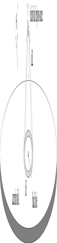
We consider now a self-consistent model where Inverse Compton process takes place on soft photons from the accretion disk, which are themselves emitted as thermal radiation due to the heating of the disk by hard radiation. The disk is modelized by an infinite slab radiating isotropically like a black-body at the same equilibrium temperature (Fig. 1). The high energy source is assumed to be an optically thin plasma of highly relativistic leptons, at rest at a given distance $Z_{0}$ above the disk axis. Its size is small enough to be considered as a point source. We consider a Euclidean geometry so that there is no curvature of photon geodesics. The general relativistic case will be studied in an accompanying paper (Petrucci & Henri 1997). The particle distribution is assumed to be isotropic. As long as the disk emission is concerned, there is no need to specify the energy distribution giving rise to IC process. However, the spectrum of high energy radiation will be determined by this distribution. This will be developed in section 4.

3.2 The self consistent solution

We shall see now that the above problem admits in fact a unique self-consistent solution in conveniently scaled variables. For a given disk emissivity, the power emitted per unit solid angle by the high energy source is given by Eq. (38), where $g(\mu)=1/2$ and the Eddington parameters are to be calculated with the disk emissivity. Integrating over solid angle, one gets the total high energy luminosity:

$$L_{t}=\frac{16\pi}{3}\sigma_{T}N\langle\gamma^{2}\rangle J.$$ (50)

Thus, the power per unit angle can be expressed as:

$$\frac{dP}{d\Omega}=\frac{3L_{t}}{32\pi}\mbox{$F_{\eta\chi}(\mu)$}.$$ (51)

The Eddington coefficients can be at turn calculated if one knows the disk emissivity. Under the hypothesis that the disk reprocesses the whole radiation impinging on it, it is determined by equating the power absorbed and emitted by a surface element $dS$ of the disk at a radius $r$ (cf. Fig. (1)):

$$F(r)dS=\frac{dP}{d\Omega}d\Omega=\mu^{\prime 3}\frac{dP}{d\Omega}\frac{dS}{Z_{0}^{2}}$$ (52)

where $\mu^{\prime}=-\mu=Z_{0}(r^{2}+Z_{0}^{2})^{-1/2}$ is the cosine of the impinging angle of radiation ($\mu^{\prime}$ varies from 1 to 0).
From equation (51) and (52), one gets:

$$F(r)=\frac{3L_{t}}{32\pi Z_{0}^{2}}F_{\eta\chi}(-\mu^{\prime})\mu^{\prime 3}$$ (53)

Under the assumption of isotropic emissivity of the disk, one gets the specific intensity due to the reemission by the disk at the radius $r$ toward the source:

$$I(\mu)=\frac{F(r)}{\pi}=\xi\mu^{3}F_{\eta\chi}(-\mu)$$ (54)

where we define the dimensionless parameter

$$\xi\equiv\frac{3L_{t}}{32\pi^{2}Z_{0}^{2}J}.$$ (55)

Inserting this expression in the definition of Eddington parameters, one gets the following linear system

$$1 = \xi(G_{0}(1-\chi)+4G_{1}\eta+G_{2}(3\chi-1))$$

$$\eta = \xi(G_{1}(1-\chi)+4G_{2}\eta+G_{3}(3\chi-1))$$ (56)

$$\chi = \xi(G_{2}(1-\chi)+4G_{3}\eta+G_{4}(3\chi-1))$$

where

$$G_{n}=\frac{1}{2}\int_{\mu_{min}}^{\mu_{max}}\mu^{n+3}d\mu=\frac{1}{2(n+4)}(\mu_{max}^{n+4}-\mu_{min}^{n+4}).$$ (57)

This homogeneous system admits a non trivial solution only if the determinant is set to zero, which gives a cubic equation in $\xi$. One can then determine the angular parameters $\eta$ and $\chi$, and the emitted flux with Eq. (53). In the case of an infinite slab, one gets simply $G_{n}=\displaystyle\frac{1}{2(n+4)}$. The numerical solutions of the cubic equation are then $\xi=$ 1.449, 48.136 and 7786.45. Only the first one is compatible with the physical constraints $\eta\leq 1$, $\chi\leq 1$. The solutions of the system are approximately $\eta=0.82288$ and $\chi=0.69957$.
With these values, the high energy emissivity has the following universal angle dependence:

$$\frac{dP}{d\Omega}(\mu)=L_{t}(0.0686-0.0982\mu+0.0328\mu^{2}),$$ (58)

and thus the illuminated disk has the corresponding emissivity law:

$$F(r) = \sigma T_{eff}^{4}(r)$$ (59)

$$= \frac{L_{t}Z_{0}}{(Z_{0}^{2}+r^{2})^{3/2}}\times$$

$$\left(0.0686+\frac{0.0982}{\left(1+\left(\frac{r}{Z_{0}}\right)^{2}\right)^{1/2}}+\frac{0.0328}{1+\left(\frac{r}{Z_{0}}\right)^{2}}\right).$$

The total disk luminosity is

$$L_{disk} = \int_{0}^{\infty}2\pi rF(r)dr=L_{t}\frac{4+3\eta}{8}$$

$$\simeq 0.8086L_{t}.$$

It represents thus the main part of the total bolometric luminosity $L_{t}$.

3.3 Disk emission spectrum

Under the assumption of isotropic blackbody emission, without limb darkening, the emitted spectrum, integrated over angles, can be written as

$$L_{\nu}=\int_{r_{min}}^{r_{max}}\pi B_{\nu}(T_{eff})2\pi rdr$$ (61)

where the effective temperature $T_{eff}$ is defined in equation (59) and $\displaystyle B_{\nu}(T)=\frac{2h\nu^{3}}{c^{2}}\left[exp\left(\frac{h\nu}{k_{B}T_{eff}(r)}\right)-1\right]^{-1}$ is the usual Planck source function. Introducing the characteristic variables:

$$T_{c} \equiv \left(\frac{3L_{t}}{32\pi\sigma Z_{0}^{2}}\right)^{1/4}$$ (62)

$$\nu_{c} \equiv k_{B}T_{c}/h$$ (63)

and defining the following reduced variables:

$$\overline{T} = T/T_{c}$$

$$\overline{\nu} = \nu/\nu_{c}$$ (64)

$$\overline{L}_{\overline{\nu}} = \frac{\nu_{c}}{L_{t}}L_{\nu},$$

one can write the emitted spectrum in the universal form:

$$\overline{T}(\mu^{\prime}) = \mu^{{}^{\prime}3/4}F_{\eta\chi}(-\mu^{\prime})^{1/4}$$ (65)

$$\overline{L}_{\overline{\nu}} = \frac{45\overline{\nu}^{3}}{16\pi^{4}}\int_{\mu^{\prime}_{min}}^{\mu^{\prime}_{max}}\mu^{{}^{\prime}-3}\left[\exp\left(\frac{\overline{\nu}}{\overline{T}(\mu^{\prime})}\right)-1\right]^{-1}d\mu^{\prime}.$$ (66)

It is interesting to compare this spectrum with that of a standard SS accretion disk. The flux emitted by a SS disk with a null torque at the inner radius $r_{i}$ is given by

$$F(r)=\sigma T^{4}_{eff,SS}(r)=\frac{3r_{i}L_{disk}^{(SS)}}{2\pi r^{3}}\left(1-\left(\frac{r_{i}}{r}\right)^{1/2}\right).$$ (67)

For large $\nu$, emitted at large distances, the spectra have the same slope, with the dependence $L_{\nu}\propto\nu^{1/3}$. This is because the release of gravitational energy and the illumination by a central source give rise to the same dependence of the energy flux at large distance $F(r)\propto r^{-3}$.
Inspection of formulae (53), (3.2) and (67) show that the low frequency luminosity will be the same for both models if

$$\frac{L_{disk}}{L_{disk}^{(SS)}}=\frac{2(4+3\eta)}{(3-\chi)}\left(\frac{r_{i}}{z_{0}}\right)$$ (68)

For a Schwarzschild black hole with a mass $M$, $r_{i}=6GM/c^{2}$.

Figure 2: Spectra of the present illumination model for an infinite slab (plain line) and a standard SS accretion disk in reduced units (see text for definitions). The 2 spectra are normalized in order to have the same low frequency flux

Figure 3: Radial temperature profile of the present illumination model for an infinite slab (plain line) and a standard SS accretion disk (dashed line). The 2 curves are also normalized in order to have the same asymptotic behaviors for $r\rightarrow\infty$

For comparison, we have chosen $Z_{0}=70GM/c^{2}$. Figure (2) represents the exact spectrum emitted by the disk in our illumination model, with $\mu^{\prime}_{min}=0$ and $\mu^{\prime}_{max}=1$, and in the standard SS model. Figure (3) represents the corresponding radial temperature profile for both models. As one can see, in the illumination model, the temperature stops rising at a distance $r\sim Z_{0}$ whereas it keeps growing in the standard accretion disk model, where most of accretion energy is released at the smallest radii. As a consequence, for the same low frequency flux, the illumination model predicts a lower bolometric luminosity, and peaks at a lower frequency than the standard SS model.

3.4 Ratio of high energy to disk emission

The model predicts also a definite ratio between the high energy IC luminosity and the disk thermal emission; the total (non intercepted) IC luminosity is emitted in the upper hemisphere ($0\leq\mu\leq 1$), whereas the disk luminosity is equal to the IC luminosity in the lower hemisphere ($-1\leq\mu\leq 0$). From equation (51), one gets

$$R = \frac{L_{he}}{L_{disk}}=\frac{\int_{0}^{1}\frac{dP}{d\Omega}2\pi d\mu}{\int_{-1}^{0}\frac{dP}{d\Omega}2\pi d\mu}$$ (69)

$$= \frac{1-3\eta/4}{1+3\eta/4}$$

One has $R\sim 0.237$ for an infinite plane. One can also evaluate the ratio between the apparent disk and high energy luminosities in a given direction of observation $\mu_{0}$. It is given by:

$$R(\mu_{0}) = \frac{\pi(dP/d\Omega)_{IC}}{\mu_{0}L_{disk}}$$ (70)

$$= \frac{3F_{\eta\chi}(\mu_{0})}{4\mu_{0}(4+3\eta)}.$$

Figure 4: Ratio of high energy to soft energy luminosity as a function of inclination angle, in logarithmic scale. The disk is modeled by an infinite slab

This function is displayed in Fig. (4). It presents a minimum on the disk axis ($\mu_{0}=1$), both because the disk emission is maximal at small inclination angle, and IC is minimal because of the soft photon anisotropy. Thus, the model predicts that the observed X/UV ratio is smaller than 1 for $\mu_{0}\geq 0.2$, and can be as low as 0.012.

4 Application to AGN

4.1 The high energy spectrum

As reminded in the introduction, the high energy emission of Seyfert galaxies can be well reproduced by a primary power-law spectrum with a spectral index $\alpha\simeq 0.9$, superimposed on more complex structures, that can be produced by the reflection of the hard X-rays on a cold surface. Although the precise modeling of such a reflection component is beyond the scope of this paper, it is clearly compatible with the above picture. The primary power-law emission should be associated with the emission from the hot source, and the UV-optical component (Blue Bump) associated with the reprocessed radiation, together with a Compton backscattered component in X-rays (not taken into account in the present model). Noticeably, this power law is exponentially cut-off above a characteristic energy of about 100 keV, with some uncertainty its precise value. Contrarily to thermal models, where this cut-off is related to the temperature of the hot comptonizing plasma, we propose to interpret it as a high energy cut-off of the relativistic energy distribution. If the UV bump is located around 10 eV, this gives an cut-off Lorentz factor $\gamma_{0}\sim 10^{2}$. Although a detailed model of the high energy source is again out of the scope of this work, one can note that a model associating pair production and pair reacceleration can provide such upper cut-off, to avoid catastrophic run-away pair production (Done et al. [1990] ; Henri & Pelletier [1991] ).
To account for the high energy cut-off, we will assume that the particles (electrons or positrons) energy distribution function (integrated over volume) has the form:

$$n(\gamma)=N_{0}\gamma^{-s}\exp\left(-\frac{\gamma}{\gamma_{0}}\right),\ \gamma_{min}<\gamma<\gamma_{max}$$ (71)

Inserting this function in Eq. (43), noting that $f(\gamma,\mu)=n(\gamma)/2$, one gets the expression of high energy specific power:

$$\frac{dP}{d\Omega d\nu} = \frac{N_{0}\sigma_{T}}{4}J\mbox{$F_{\eta\chi}(\mu)$}\left(\frac{\langle\epsilon_{s}\rangle A(\mu)}{h}\right)^{(s-3)/2}\nu^{-(s-1)/2}\times$$ (72)

$$\exp\left(-\left(\frac{\nu}{A(\mu)\nu_{0}}\right)^{1/2}\right)$$

where $\nu_{0}=\gamma_{0}^{2}\langle\epsilon_{s}\rangle/h$ is a high energy frequency cut-off.
Integrating Eq. (38) over all angles, one can also write the total high energy luminosity as:

$$L_{t}=\frac{16\pi}{3}C_{0}N_{0}\sigma_{T}J\gamma_{0}^{(3-s)}$$ (73)

where $C_{0}$ is expressed as an incomplete gamma function:

$$C_{0}=\int_{\gamma_{min}/\gamma_{0}}^{\gamma_{max}/\gamma_{0}}x^{2-s}\exp(-x)dx=\Gamma(3-s;\gamma_{min}/\gamma_{0};\gamma_{max}/gamma_{0})$$ (74)

One can also evaluate the mean photon energy

$$\langle\epsilon_{s}\rangle=\frac{J}{\mbox{$\overline{J}$}}=C_{1}h\nu_{c}$$ (75)

where

$$C_{1}=\frac{8\zeta(4)}{3\xi\zeta(3)\int_{\mu_{min}}^{\mu_{max}}\mbox{$\overline{T}(\mu)$}^{3}d\mu}$$ (76)

where $\zeta(n)$ is the Riemann Zeta function. One can finally compute the photon number anisotropy parameter $\overline{\eta}$, appearing in the computation of $A(\mu)$ (cf. Eq. (33)):

$$\mbox{$\overline{\eta}$}=\frac{\mbox{$\overline{H}$}}{\mbox{$\overline{J}$}}={\frac{\int_{\mu_{min}}^{\mu_{max}}\mu\mbox{$\overline{T}(\mu)$}^{3/4}d\mu}{\int_{\mu_{min}}^{\mu_{max}}\mbox{$\overline{T}(\mu)$}^{3/4}d\mu}}.$$ (77)

remembering that the specific intensity emitted by the disk is supposed to be the Planck function. For $\mu_{min}=0$ and $\mu_{max}=1$, one gets $C_{1}\simeq 3.41$ and $\mbox{$\overline{\eta}$}\simeq 0.788$ Using the reduced variables defined by Eq. (64), one gets finally the following expression for the high energy specific power:

$$\frac{d\overline{P}}{d\Omega d\overline{\nu}} = \frac{3\gamma_{0}^{s-3}}{64\pi C_{0}}\left(C_{1}A(\mu)\right)^{(s-3)/2}\overline{\nu}^{(1-s)/2}\times$$

$$\mbox{$F_{\eta\chi}(\mu)$}\exp\left[-\left(\frac{\overline{\nu}}{A(\mu)\overline{\nu}_{0}}\right)^{1/2}\right]$$

with $\overline{\nu}_{0}=\nu_{0}/\nu_{c}$. Noticeably, the high energy cut-off depends on the inclination angle, the smallest angles giving the lowest cut-off.

Figure 5: Broad band spectra for various inclination angles, in reduced units. The values of parameters are the following: $s=3$, $\overline{\nu}_{0}=10^{4}$

4.2 Validity of the point source approximation

It is obvious that a point source is a convenient, but unrealistic approximation of the real geometry of the source, since it has a zero cross section and a infinite Thomson opacity. Rather, for a given number $N$ of scattering particles, one gets a minimal size $R_{min}$ for the source being optically thin; for a homogeneous sphere, it requires

$$R\geq R_{min}=\left(\frac{3N\sigma_{T}}{4\pi}\right)^{1/2}$$ (79)

This hot source will sustain a solid angle $\Omega\simeq\pi(R_{min}/Z_{0})^{2}$. The total number of particles in the optically thin regime can be calculated by Eq. (55) and (50), which yields:

$$N=\frac{2\pi Z_{0}^{2}\xi}{\sigma_{T}\langle\gamma^{2}\rangle}$$ (80)

Using the distribution function given by Eq. (71), one gets

$$\langle\gamma^{2}\rangle=\gamma_{0}^{2}\frac{\Gamma(3-s;\gamma_{min}/\gamma_{0};\gamma_{max}/\gamma_{0})}{\Gamma(1-s;\gamma_{min}/\gamma_{0};\gamma_{max}/\gamma_{0})}$$ (81)

Combining Eq. (79), (80) and (81), one obtains a estimate of the minimal radius of the source:

$$\frac{R_{min}}{Z_{0}}=\frac{1}{\gamma_{0}}\left(\frac{3\xi\Gamma(1-s;\gamma_{min}/\gamma_{0};\gamma_{max}/\gamma_{0})}{2\Gamma(3-s;\gamma_{min}/\gamma_{0};\gamma_{max}/\gamma_{0})}\right)^{1/2}$$ (82)

Figure 6: Contour plot of the minimal angular size of the source $R_{min}/Z_{0}$, as a function of the spectral index $s$ and the cut-off Lorentz factor $\gamma_{0}$. The limits of the particle energy distribution are $\gamma_{min}=1$ and $\gamma_{max}=\infty$

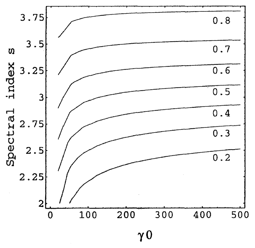
Figure (6) represents the contour plot of $R_{min}/Z_{0}$ as a function of $\gamma_{0}$ and $s$, for $\gamma_{min}=1$ and $\gamma_{max}=\infty$. As we have mentioned, high energy observations of Seyferts seem to favour values of $\gamma_{0}\simeq 10^{2}$, and $s\simeq 3$. This corresponds to $R/Z_{0}\simeq 0.5$, which means that the hot source is not really point-like, but moderately extended: it could be realized by a region with a radius $R\sim 15r_{g}$, located around $Z_{0}\sim 30r_{g}$. These values seem reasonable for a shock in the inner region of a jet emitted by an accretion disk. Of course, a correct treatment should take into account the finite size of the source, but the calculations are much more involved if the particles are off-axis: the present theory must be considered as a preliminary one, and the application to the extended case will be treated in a future work.

4.3 Application to broad-band spectra.

Figure (5) represents the overall spectra predicted by the model for different inclination angles, ranging from $\theta_{0}=0^{\circ}$ to $60^{\circ}$. For all these angles, the X-ray luminosity is apparently smaller than the UV bump. Higher inclination angles will probably lead to strong absorption through the external parts of the disk, presumably a molecular torus: in the unification scheme, they would correspond to Seyfert 2 galaxies (but see below). The UV/X ratio depends markedly on the inclination angle: noticeably, the smaller ratio correspond to almost face-on objects. The upper energy cut-off is also lightly angle dependent, due to the $A(\mu)$ factor in Eq. (4.1). Face-on objects have the lowest cut-off.
Direct comparison with observations is difficult at this stage, because the model does not include other important components, like the absorption edge, the Compton reflection feature and the fluorescent Fe K$\alpha$ line that are observed in many Seyferts. Without detailed calculations, it can be expected however that these components are more pronounced that those predicted by an isotropic illumination model, the mean enhancement factor being of the order of $R^{-1}\simeq 4$ (Eq. (69)). Ginga and more recent ASCA observations (Nandra et al. [1997]) have found large equivalent widths for the Fe K$\alpha$ line, with a mean value around $230\pm 60$ eV, but up to $550^{90}_{-120}$ eV for NGC 4151, whereas detailed calculations of George and Fabian ([1991]) and Matt et al. ([1991]) predicted a value around 140 eV. These results depend however on the ionization state of the matter (Matt et al. [1993]) and the assumed iron abondance (Reynolds et al. [1995]). Clearly more work must be done to clarify this issue.
The resolved line profiles seen by ASCA can be well fitted by an illuminated accretion disk in rotation around a black hole, with $\simeq 50$ per cent of the line emission originating within $\simeq 20$ $r_{g}$, and $\simeq 80$ per cent within $\simeq 100$ $r_{g}$(Nandra et al. [1997]): this is thus compatible with a hot source located at a few ten $r_{g}$ above the disk.
Although a precise prediction of UV/X flux is difficult to assess, we have used the work of Walter & Fink ([1993]), who compared the X and UV flux in a large sample of Seyfert 1 galaxies, to make a rough comparison with our model. We assumed that the $1375$ $\AA$ flux is close to the maximum of the UV bump, whereas the 2 keV flux is not strongly contaminated by the soft excess or the reflection component, and is representative of the low energy part of the hard X-ray spectrum given by Eq. (72). We thus consider the apparent UV/X ratio $R_{a}$ of these two values.
In our model, the maximum of the UV bump is found numerically to be $\overline{\nu}\overline{L}_{\overline{\nu},max}\simeq 0.419$ at ${\overline{\nu}}\simeq 4$. With the geometrical factor due to disk inclination, one gets thus

$$\overline{\nu}\frac{d\overline{P}_{UV}}{d\Omega d\overline{\nu}}(\mu)\simeq\frac{0.419}{\pi}\mu$$ (83)

The hard X-ray flux at low energy is given by Eq. (72) with $\overline{\nu}\ll{\overline{\nu_{0}}}$ Taking $s=3$ for simplicity, one gets

$$\overline{\nu}\frac{d\overline{P}_{X}}{d\Omega d\overline{\nu}}(\mu)\simeq\frac{3\mbox{$F_{\eta\chi}(\mu)$}}{64\pi C_{0}}$$ (84)

, so that:

$$R_{a}(\mu)\simeq 9.05\frac{\mu C_{0}}{\mbox{$F_{\eta\chi}(\mu)$}}$$ (85)

Now for a sample of $N_{g}$ galaxies oriented randomly between $\mu=0$ and $\mu=1$, one expects a uniform distribution

$$\frac{dN}{d\mu}=N_{g}$$ (86)

One gets the probability distribution of the UV/X ratio $R_{a}$:

$$\frac{dP}{dR_{a}}=\left|\frac{d\mu}{dR_{a}}\right|=\frac{\mbox{$F_{\eta\chi}(\mu)$}^{2}}{9.05C_{0}(3-\chi-(3\chi-1)\mu^{2})}$$ (87)

Figure 7: Comparison of the probability distribution of apparent UV/X ratio $R_{a}$ compiled by Walter and Fink([1993]) and the predicted values, with $\gamma_{0}=10^{2}$

Figure (7) represents the comparison of observed and predicted probability distribution of the apparent UV/X ratio $R_{a}$, for $\gamma_{0}=10^{2}$. To derive the probability density $dP/dR_{a}$, the observed values have been binned into intervals of width 5, and statistical error bars have been added. The agreement is very satisfactory, which can be rather fortuitous in view of the approximations used.
Although the widespread opinion, based on unification models, is that Seyfert 1 galaxies are seen nearly pole-on, whereas Seyfert 2 are their edge-on counterparts, there is some evidence that the reality may be more complex. In a statistical study of the 48 Seyfert galaxies from the CfA catalog, Edelson et al. ([1987]) concluded that all Seyfert 2, but only one third of Seyfert 1, present an excess at 60 $\mu m$, attributed to thermal emission from dust. Since emission from dust is not expected to be highly anisotropic, it would imply that the unification model applies only to a subclass of objects, which possess an obscuring torus with some opening angle. The other subclass could not possess this torus, and give only Seyfert 1 galaxies seen under any inclination angle. This could explain the presence of high inclination angles, i.e. low UV/X ratios galaxies. But of course, a large intrinsic or extrinsic absorption could change a lot this picture.

4.4 Scaling laws

As is well known, a usual assumption for the mass-luminosity ratio of AGN is that the bolometric luminosity is limited by the radiation pressure to the Eddington luminosity:

$$L_{E}=\frac{4\pi GMm_{p}c}{\sigma_{T}}.$$ (88)

This relationship predicts a linear correlation between mass and luminosity for Eddington accreting black-holes, $L\propto M$; the corresponding Eddington temperature is given by

$$T_{E}=\left(\frac{L_{t}}{4\pi r_{g}^{2}}\right)^{1/4}\propto M^{-1/4}.$$ (89)

We show here that the present model predicts different scaling laws, if one adds some supplementary assumptions on the physics of the hot source. At first sight, all equations of the models are linear with respect to the global luminosity, so no particular relationship is predicted between the luminosity and other parameters like $M$ or $Z_{0}$. However things are different if one considers the microphysics and a realistic geometry of the hot source. First, let us consider again the upper energy cut-off of the IC spectrum discussed in Paragraph (2.4). Observations seem to show that all Seyfert galaxies have the cut-off around the same value, approximately 100 keV; however, when taking into account the reflection component, this estimate could be somewhat higher, up to 400 keV (Zdziarski et al. [1995]). This is sufficiently close to pair production threshold to make plausible the idea that this cut-off is in some way fixed by a regulation mechanism to avoid run-away pair production. In this case, the cut-off energy is a physical quantity, determined by microphysics rather that macrophysical quantities. The maximal energy of photons produced by IC process is of the order

$$\gamma_{0}^{2}h\nu_{c}\approx constant.$$ (90)

Now it is plausible that the size of the source and its distance to the black hole are controlled by the global environment responsible for the hot source. Conceivably, it could be realized through a strong shock terminating an aborted jet. If one makes the (admittedly crude) assumption that all distances scale like the hole radius $r_{g}$, then one gets $R/Z_{0}\approx constant$. For a given spectral index $s$, Eq. (82) predicts $\gamma_{0}\approx constant$, and Eq. (90) gives $\nu_{c}\approx constant$. Finally one gets the following scaling laws:

$$T_{c} \propto \nu_{c}\propto M^{0}\approx constant$$ (91)

$$L_{t} \propto M^{2}.$$ (92)

that is , the temperature of the Blue Bump does not depend on the mass and the luminosity scales like the square of the mass. Of course, one could observe substantial variations of at least one of these quantities if $s$ or $\Omega$ varies, either by a variation of $Z_{0}$ or a variation of $R$. Interestingly, observations seem to corroborate these behaviors: on a sample of many quasars and galaxies spanning a large range of masses, Walter & Fink ([1993]) found that the Blue Bump and soft X-ray excess were approximately in the same ratio, although the central masses can differ by a factor $10^{4}$. This is very hard to explain in the frame of conventional accretion models. In another study, using a specific model to describe the width of Broad Lines from the emission by the external part of the disk, Collin-Souffrin & Joly ([1991]) have deduced the inclination angles and central masses of a sample of Seyfert 1 galaxies and quasars. They found a correlation between mass and luminosity under the form $L\propto M^{\beta}$, with $\beta=1.8\pm 0.6$. Although these results have been obtained on a limited sample, they are compatible with the previous results and clearly different from those predicted by the standard accretion disk models. A rather intriguing consequence is that there is a maximal mass above which the accretion becomes impossible by such a mechanism, where the luminosity predicted by Eq. (92) gets higher than the Eddington luminosity. From Eq. (62) and (75), the total luminosity can be written under the form:

$$L_{t}=\frac{256\pi^{6}G^{2}}{45C_{1}^{4}h^{3}c^{6}}\left(Z_{0}/r_{g}\right)^{2}M^{2}\langle\epsilon_{s}\rangle^{4}$$ (93)

Comparing with Eq. (88), one finds that $L_{t}=L_{edd}$ for

(94)

This value is surprisingly close to that commonly invoked for the most luminous known quasars, which apparently accrete at a near-Eddington rate. It is however unclear how accretion would be stopped for higher central masses, since the radiation pressure can be effective only if the central engine actually radiates.

5 Conclusion

We have shown that a model based on reillumination of a disk by an anisotropic IC source could lead to a self-consistent picture where the angular distribution of high energy radiation and the radial temperature distribution of the disk are mutually linked and both determined in a single way. The model offers a simple explanation for the correlated long term variability of X and UV radiation, the short term variability of X-rays non correlated with UV variations, and the apparent X/UV deficit that seems contradictory with simple reillumination models. In its simplest form, it predicts a unique shape of disk spectrum and a X/UV ratio depending only on the inclination angle. The predicted values are in good agreement with observations. In an accompanying paper (Petrucci & Henri [1997]), we shall study the influence of relativistic corrections on the above scheme to account for the gravitational effect of a Schwarzschild or a Kerr black hole. A precise comparison with real spectra should also include other components, such as a reflection component and a fluorescent Fe K$\alpha$ line. This is deferred to a future work.

References

- [1984] Begelman M.C., Blandford R.D., Rees M.J., 1984, Rev. Mod. Phys. 56, 255
- [1992] Clavel J. et al. 1992, ApJ, 393, 113
- [1991] Collin-Souffrin S., Joly M., 1991, Disks and Broad Line Regions. In: Duschl W.J., Wagner S.J. (eds) Physics of Active Galactic Nuclei. Springer-Verlag, p. 195
- [1995] Dermer C.D., Gehrels N., 1995, ApJ 447, 103
- [1992] Dermer C.D., Schlickeiser R., 1992, Science 257, 1642
- [1990] Done C., Ghisellini G., Fabian A. C., 1990, MNRAS 245, 1
- [1987] Edelson R.A., Malkan M.A., Rieke G.H., 1987, ApJ 321, 233
- [1993] Field G.B., Rogers R.D., ApJ 403, 94
- [1991] George I.M., Fabian A.C., 1991, MNRAS 249, 352
- [1991] Ghisellini G., George I.M., Fabian A.C., Done C., 1991, MNRAS 248, 14
- [1991] Haardt F., Maraschi L., 1991, ApJ 380, L51
- [1993] Haardt F., Maraschi L., 1993, ApJ 413, 507
- [1995] Haardt F., Maraschi L., Ghisellini G., 1995, ApJ 432, L95
- [1991] Henri G., Pelletier G., 1991, ApJ 383, L7
- [1992] Jourdain E., et al., 1992a, A&A 256, L38
- [1988] Lightman A.P., White T.R., 1988, ApJ 335, 57
- [1993] Maisack M., et al., 1993, ApJ 407, L61
- [1993] Marcowith A., Henri G., Pelletier G., 1995, MNRAS 277, 681
- [1991] Matt G., Perola G.C., Piro L., 1991, A&A 247, 27
- [1993] Matt G., Fabian A.C., Ross R.R., 1993, MNRAS 262, 179
- [1994] Nandra K., Pounds K. A., 1994, MNRAS 268, 405
- [1997] Nandra K., et al., 1997, ApJ 477, 602
- [1986] Perola G.C., et al., 1986, ApJ 306, 508.
- [1997] Petrucci P.O., Henri G., 1997, A&A, in press.
- [1990] Pounds K.A., et al., 1990 , Nat 344, 132
- [1992] Punch M., et al., 1992, Nat 358, 477
- [1995] Reynolds C.S., Fabian A.C., Inoue H., 1995, MNRAS 276, 1311
- [1996] Quinn J., et al., 1996, ApJ 456, L83
- [1973] Shakura N.I., Sunayev R.A., 1973, A&A 24, 337
- [1996] Svensson R., 1996, A&AS, in press.
- [1995] von Montigny C., et al., 1995, ApJ 440, 525
- [1993] Walter R., Fink, H.H., 1993, A&A 274, 105
- [1995] Weaver K.A., Arnaud K.A., Mushotzky R.F., 1995, ApJ 447, 121
- [1990] Zdziarski A.A., Ghisellini G., George I.M., Svensson R., Fabian A.C., Done C., 1990, ApJ 363, L1
- [1995] Zdziarski A. A., Johnson W.N., Done C., Smith D., McNaron-Brown K., 1995, ApJ 438, L63