Anisotropic illumination of AGN’s accretion disk by a non thermal source . II General relativistic effects

Abstract

In a previous paper (Henri & Petrucci [submitted], hereafter paper I), we have derived a new model in order to explain the UV and X-ray emission of radio quiet AGNs. This model assumes that a point source of relativistic leptons ($e^{+},e^{-}$) illuminates the accretion disk of the AGN by Inverse Compton process. This disk is supposed to be simply represented by a finite slab which radiates only the energy reprocessed from the hot source. The radiation field within the hot source region is therefore highly anisotropic, which strongly influences the Inverse Compton process. The different Eddington parameters characterizing the radiative balance of this system have been calculated self-consistently in the Newtonian case (paper I) giving a universal spectrum for a given inclination angle. In this paper, we take into account relativistic effects by including the gravitational redshift, the Doppler boosting and the gravitational focusing due to the central supermassive black hole. This has the effect of modifying the radial temperature profile in the innermost region of the disk (at some gravitational radii). However, the spectrum is hardly different from that obtained in the Newtonian case, unless the hot source is very close to the black hole. These results are clearly different from standard accretion disk models where the gravitational energy is mainly released in the vicinity of the black hole.

1 Introduction

It is now generally agreed that the engine of high power emission in AGNs is a supermassive black hole of $10^{6}-10^{9}\,M_{\sun}$, accreting matter from a surrounding accretion disk (Shakura & Sunyaev [1973]; Rees [1984]). Besides, several satellites observations of radio quiet Seyfert galaxies have allowed to obtain an average high energy (X-ray/$\gamma$-ray) spectrum, better reproduced by a complex superposition of a primary power law, a reflected component from a cold thick gas, a fluorescent iron K line and an absorption by a hot medium (Pounds et al. [1990]). On the other hand, Clavel et al. ([1992]) have shown a close simultaneity between UV and optical variations of some Seyfert galaxies, which cannot be reproduced by standard accretion disk models. Rather, these results are better explained if the UV-optical emission comes from the reprocessing of hard radiation emitted by a hot source above the disk. In paper I, we have proposed a new model involving a point source of relativistic leptons (the hot source) emitting hard radiation by Inverse Compton (IC) process on soft photons produced by the accretion disk. The disk itself radiates only through the reprocessing of the hard radiation impinging on it. Such a geometry is highly anisotropic, which takes a real importance in the computation of IC process (Ghisellini et al. [1991] ; paper I). Paper I dealt only with the Newtonian case and did not include the relativistic effects: these are first, the Doppler shift due to the rotation of the disk; second the gravitational shift, undergone by photons which follow a null geodesic, either from the disk to the hot source and inversely, or from the AGN to the observer at infinity; and third, the gravitational focusing, most important for rays of light skimming the black hole. Thus, the subject of this paper (paper II) is to extend this simple model to the general relativistic formulation appropriate to a Kerr black hole. The organization is as follows. We will establish, in section 2, the general equations which govern the radiative balance between the hot source and the accretion disk in an axisymmetric gravitational field. We will study the case of a rotating black hole in the Kerr metrics in section 3. In section 4, we will finally obtain the power spectra emitted by this model for different values of the inclination angles and the height of the hot source, and conclude on the importance of the gravitational effects on the overall spectrum.

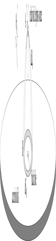
Figure 1: The general picture of the model. We have also drawn the trajectory of a beam of photons emitted by the hot source in a solid angle $d\Omega_{A}$ and absorbed by a surface ring $dS_{B}$ on the disk. The letters A and B refer to the indices define in part (2.1)

2 Relativistic energy balance equations

The geometry of the system, formed by the hot source and the accretion disk, is sketched in Fig. 1. The energy balance can be solved self-consistently, for a given disk emissivity law. Actually, the emission of the disk is entirely controlled by the hard radiation angular distribution, which is at turn determined by the disk emissivity through the anisotropic IC process. In paper I, we solved the Newtonian case of this radiative balance by solving a system of 3 equations between the 3 Eddington parameters characterizing the photon field. When relativistic effects are taken into account, the same principle can be used, but with some modifications. First, the photons do not follow any more straight trajectories, but geodesics whose equations must be deduced from the metrics. Second, one must take care of gravitational and Doppler shifts between the hot source, the rotating accretion disk and the observer at infinity.

2.1 The different frames

The Kerr metrics describes the exterior metrics of an stationary axisymmetric gravitational field around a rotating body. It is completely specified by its total mass $M$ and angular momentum per unit mass $a$. The line element can be written in Boyer-Lindquist coordinates as follows (we use convenient units such that $c=G=1$; then the unit length is $GM/c^{2}=R_{g}/2=M$, $R_{g}$ being the Schwarzschild radius):

$$ds^{2}=-e^{2\nu}dt^{2}+e^{2\psi}(d\phi-\omega dt)^{2}+\Delta^{-1}\Sigma dr^{2}+\Sigma d\theta^{2}$$ (1)

where

$$A = (r^{2}+a^{2})^{2}-a^{2}\Delta\sin^{2}\theta$$ (2)

$$\Delta = r^{2}+a^{2}-2Mr$$ (3)

$$\Sigma = r^{2}+a^{2}\cos^{2}\theta$$ (4)

$$e^{2\nu} = A^{-1}\Delta\Sigma$$ (5)

$$e^{2\psi} = A\Sigma^{-1}\sin^{2}\theta$$ (6)

$$w = 2aMrA^{-1}.$$ (7)

Yet, as shown by Bardeen et al. ([1972]), physics is not simple in the Boyer-Lindquist coordinate frame. First, the dragging of inertial frame becomes so severe as we approach the Kerr black hole, that the line element $ds^{2}$ goes time-like. Second, the metrics is non-diagonal which introduces algebraic complexities. For those reasons, Bardeen introduced the locally non-rotating frames (LNRF, Bardeen et al. [1972]) to cancel out, as much as possible, the “frame dragging” effects of the hole rotation. They are linked to observers whose world lines are $r=constant$, $\theta=constant$ and $\phi=\omega t+constant$. We will used the same method here. We defined the set of frames $\Re$ as these LNRF. For a Schwarzschild black hole, they correspond simply to the curvature coordinates frame $(r,\ \theta,\ \phi)$. We also define the set of frames $\Re^{*}$ which locally rotate with the disk. All terms computed in these frames are labeled with a star.
The quantities expressed at the hot source location ($\theta=0,\ r=Z_{0}$) are indexed with an A. They are indexed with a B when they are computed on the surface of the disk ($\theta=\frac{\pi}{2}$). For example, a differential elementary surface of the disk, expressed in the rotating frame $\Re^{*}$, will be noted $dS^{*}_{B}$ (cf. Fig. 1). The gravitational shift between any point P and Q is noted $(1+z)_{PQ}=\displaystyle\frac{(1+z_{P\infty})^{PQ}}{(1+z_{Q\infty})^{PQ}}$, with $(1+z_{P\infty})^{PQ}\equiv\lambda_{o}-\lambda_{e}$, $\lambda_{e}$ being the emitted wavelength of a photon and $\lambda_{o}$ the observed wavelength at infinity along the geodesic connecting $P$ and $Q$.

2.2 Computation of the specific intensity

The radiative balance between the energy radiated by the disk and that radiated by the hot source of relativistic leptons gives the relation:

$$F^{*}(r_{B}) = \frac{dP^{*}_{B}}{dS^{*}_{B}}$$ (8)

$$= (1+z)^{2}_{B^{*}A}\left(\frac{dP_{A}}{{d\Omega}_{A}}{{d\Omega}_{A}}\right)\frac{1}{dS^{*}_{B}}.$$

Here, $F^{*}(r_{B})$ is the flux emitted in the frame rotating with the disk, by the surface ring which radius is in the range [$r_{B}$,$r_{B}+dr_{B}$], and we use the fact that the ratio $\displaystyle\frac{dP_{Q}}{(1+z_{Q\infty})^{2}}$ (where $dP_{Q}$ is the radiative power, measured in $Q$, released by the hot source) is a relativistic invariant. Using, now, the covariance of the space-time quadrivolume between the 2 inertial frames $\Re$ and $\Re^{*}$, we obtain:

$$\underbrace{{dS^{*}_{B}}{dt^{*}_{B}}{dh^{*}_{B}}}_{\rm{in\ }\Re^{*}}=\underbrace{{dS_{B}}{dt_{B}}{dh_{B}}}_{\rm{in\ }\Re}$$ (9)

where $dh^{*}_{B}$ and $dh_{B}$ are the elementary space intervals in the Z direction. Since there is no motion along this direction, $dh^{*}_{B}=dh_{B}$ and thus , combining Eqs. (8) and (9), one gets:

$$F^{*}(r_{B}) = \left(\frac{dP}{{d\Omega}_{A}}{{d\Omega}_{A}}\right)\frac{1}{dS_{B}}\frac{dt^{*}_{B}}{dt_{B}}(1+z)^{2}_{B^{*}A}$$ (10)

$$= \frac{dP}{{d\Omega}_{A}}\frac{{d\Omega}_{A}}{dS_{B}}(1+z)_{BB^{*}}(1+z)^{2}_{B^{*}A}.$$

We suppose the disk to radiate isotropically like a blackbody at the temperature $T_{\rm eff}$. So, one gets also:

$$F^{*}(r_{B}) = \pi I^{*}_{B}(r_{B})$$ (11)

$$= \sigma T_{\rm eff}^{4}(r_{B}).$$ (12)

The ratio $\displaystyle\frac{dP}{d\Omega_{A}}$ of the power emitted by the hot source by solid angle unit, is derived in Eq. (48) of paper I . One gets (with $\mu_{A}=cos\theta_{A}$, cf. Fig. 1):

$$\frac{dP}{d\Omega_{A}}=\frac{3L_{t}}{32\pi J_{A}}[(3J_{A}-K_{A})-4H_{A}\mu_{A}+(3K_{A}-J_{A})\mu_{A}^{2}]$$ (13)

where $J_{A},\ H_{A}$ and $K_{A}$ are the three Eddington parameters defined by:

$$J_{A} = \frac{1}{2}\int_{-1}^{1}I(\mu_{A})d\mu_{A}$$

$$H_{A} = \frac{1}{2}\int_{-1}^{1}I(\mu_{A})\mu_{A}d\mu_{A}$$ (14)

$$K_{A} = \frac{1}{2}\int_{-1}^{1}I(\mu_{A})\mu_{A}^{2}d\mu_{A}.$$

The gravitational shifts $(1+z)_{B^{*}A}$ and $(1+z)_{BB^{*}}$ and the Jacobian $\displaystyle\frac{{d\Omega}_{A}}{dS_{B}}$ of Eq. (10) will be developed in the next section. We deduce from Eqs. (10), (11) and (13) the general expression of the specific intensity of the radiation emitted by the disk, in the rotating frame $\Re^{*}$:

$$I^{*}_{B}(r_{B}) = (1+z)^{2}_{B^{*}A}(1+z)_{BB*}\frac{d\Omega_{A}}{dS_{B}}\frac{3L_{t}}{32\pi^{2}J_{A}}\times$$ (15)

$$[3J_{A}-K_{A}-4H_{A}\mu_{A}+(3K_{A}-J_{A})\mu^{2}_{A}].$$

2.3 Computation of Eddington parameters

Now, we can find a system of 3 equations between the 3 Eddington parameters $J_{A}$, $H_{A}$ and $K_{A}$ characterizing the radiation field near the hot source. Using Eqs. (14) and (15), and the fact that $\displaystyle\frac{I}{\nu^{4}}$ is a relativistic invariant (Liouville’s theorem), one obtains:

$$J_{A} = \frac{1}{2}\int_{-1}^{1}(1+z)^{-4}_{B^{*}A}I^{*}_{B}d\mu_{A}$$

$$= \frac{1}{2}\int_{-1}^{1}(1+z)^{-2}_{B^{*}A}(1+z)_{BB*}\frac{d\Omega_{A}}{dS_{B}}\times$$

$$\frac{3L_{t}}{32\pi^{2}J_{A}}[3J_{A}-K_{A}-4H_{A}\mu_{A}+(3K_{A}-J_{A})\mu^{2}_{A}]d\mu_{A}.$$

If we define, now, the following parameters:

$$\xi_{A} = \frac{3L_{t}}{32\pi^{2}Z_{0}^{2}J_{A}}$$ (17)

$$G_{n} = \frac{1}{2}\int_{-1}^{1}(1+z)_{B^{*}A}^{-2}(1+z)_{BB*}\frac{d\Omega_{A}}{dS_{B}}Z_{0}^{2}\mu_{A}^{n}d\mu_{A},$$ (18)

we can rewrite the expression of $J_{A}$, and those of the second and third Eddington moment $H_{A}$ and $K_{A}$ in the same way, in order to obtain the following linear system:

$$\left\{\begin{array}[]{lll}J_{A}&=&\xi_{A}[J_{A}(3G_{0}-G_{2})-4H_{A}G_{1}+K_{A}(3G_{2}-G_{0})]\\ &&\\ H_{A}&=&\xi_{A}[J_{A}(3G_{1}-G_{3})-4H_{A}G_{2}+K_{A}(3G_{3}-G_{1})]\\ &&\\ K_{A}&=&\xi_{A}[J_{A}(3G_{2}-G_{4})-4H_{A}G_{3}+K_{A}(3G_{4}-G_{2})].\end{array}\right.$$ (19)

We will find the values of $\displaystyle\eta_{A}=\frac{H_{A}}{J_{A}}$ and $\displaystyle\chi_{A}=\frac{K_{A}}{J_{A}}$ by making the determinant of this system vanish, that is by solving a cubic equation in $\xi_{A}$. The only physical constraints on the choice of $\xi_{A}$ that we have to respect are $\eta_{A}\leq 1$ and $\chi_{A}\leq 1$. Note that the Newtonian case of an infinite disk of paper I can be recovered by setting $G_{n}=\displaystyle\frac{1}{2(n+4)}$. In the general case, we need to compute the values of the variables $G_{n}$, that is, to express the gravitational shifts $(1+z)_{B^{*}A}$ and $(1+z)_{BB*}$, and the ratio $\displaystyle\frac{d\Omega_{A}}{dS_{B}}$. This will be the subject of section 3 where we use the Kerr metrics to calculate explicitly these coefficients.

3 Computation in the Kerr geometry

The photons follow null geodesics either between the disk and the hot source, or between the disk/hot source and the observer at infinity. We recall the general expressions of the momentum along a null geodesic (Carter [1968], Cunningham [1975]):

$$p_{t} = -E$$ (20)

$$p_{\phi} = E\lambda$$ (21)

$$p_{r} = \pm EV_{r}^{1/2}\Delta^{-1}$$ (22)

$$p_{\theta} = \pm EV_{\theta}^{1/2}\Sigma^{-1}$$ (23)

with

$$V_{\theta} = q^{2}-(\frac{\lambda^{2}}{\sin^{2}\theta}-a^{2})\cos^{2}\theta$$ (24)

$$V_{r} = (r^{2}+a^{2}-a\lambda)^{2}-$$ (25)

$$(r^{2}+a^{2}-2r)((\lambda-a)^{2}+q^{2}).$$

$E,\ q,\ \lambda$ are constants of motion: $E$ is the energy-at-infinity and $\lambda$ and $q$ are closely related to the angular momentum. For geodesics intersecting the Z axis, one has $\lambda=0$, which is the case for every photon coming from or reaching the hot source.

3.1 The gravitational shifts

First, we need the expressions of the gravitational shifts of Eq. (18). Since the hot source A is at rest, one gets:

$$(1+z_{A\infty})^{B^{*}A}=e^{\nu_{A}}=\left(1-\frac{2MZ_{0}}{Z_{0}^{2}+a^{2}}\right)^{1/2}.$$ (26)

The shift $(1+z_{B^{*}\infty})^{B^{*}A}$ between a point $B^{*}$ rotating with the disk and the infinity, is given by Cunningham ([1975]) (with $\lambda=0$ since the geodesic crosses the hot source):

$$(1+z_{B^{*}\infty})^{B^{*}A}=e^{\nu_{B}}(1-V_{e}^{2})^{1/2}$$ (27)

where $V_{e}$ is the velocity of the disk in the locally non-rotating frame $\Re$, which can be express as a function of the coordinate angular velocity of the disk $\Omega_{e}$ (Cunningham & Bardeen [1973]):

$$V_{e} = (\Omega_{e}-\omega)e^{\psi-\nu}$$ (28)

$$\Omega_{e} = M^{1/2}(r^{3/2}+a)^{-1}.$$ (29)

We thus obtain the following expression for the gravitational shift between $A$ and $B^{*}$:

$$(1+z)_{B^{*}A}=\frac{e^{\nu_{A}}}{e^{\nu_{B}}(1-V_{e}^{2})^{1/2}}.$$ (30)

The shift between $B$ and $B^{*}$ is deduced from Lorentz transformation between the 2 inertial frames $\Re$ and $\Re^{*}$, that is:

$$(1+z)_{BB^{*}}=(1-V_{e}^{2})^{1/2}.$$ (31)

3.2 Computation of $\displaystyle\frac{d\Omega_{A}}{dS_{B}}$

The disk surface element $dS_{B}$ contained between $r_{B}$ and $r_{B}+dr_{B}$ is calculated in Appendix A:

$$dS_{B}=2\pi A^{1/2}\Delta^{-1/2}dr_{B}.$$ (32)

Thus, we obtain:

$$\frac{d\Omega_{A}}{dS_{B}}=A^{-1/2}{\Delta^{1/2}}\frac{d\mu_{A}}{dr_{B}}.$$ (33)

The derivative $\displaystyle\frac{d\mu_{A}}{dr_{B}}$ is computed numerically by integrating the equation of motion between the hot source and the disk, for a grid of initial values of $\mu_{A}$. The equation of motion has been obtained by Carter ([1968]) taking full advantage of the separation of variables:

$$\int_{0}^{\pi/2}\frac{d\theta}{\sqrt{V_{\theta}}}=\int_{Z_{0}}^{r_{B}}\frac{dr}{\sqrt{V_{r}}}.$$ (34)

The signs of $V_{r}^{1/2}$ and $V_{\theta}^{1/2}$ are always the same as the signs of $dr$ and $d\theta$, respectively. In this case, $d\theta$ is always positive (we do not take into account geodesics spinning round the black hole). Only $dr$ can change its sign at a turning point in $r$. The constant of motion $\lambda$ and $q$ must be taken such that, at the starting point A, one has:

$$p_{\phi} = 0$$ (35)

$$p_{r}p^{r} = \mu_{A}^{2}p_{t}p^{t}.$$ (36)

This gives:

$$\lambda = 0$$ (37)

$$q = \left[(1-\mu_{A}^{2})(Z_{0}^{2}+a^{2})(Z_{0}^{2}+a^{2}-2MZ_{0})^{-1}-a^{2}\right]^{1/2}.$$ (38)

Equation (34) is then solved with respect to $r_{B}$, for a given $\mu_{A}$. Once all the coefficients $G_{n}$ are computed, the linear system (19) can be solved, by making its determinant vanish. One can extract the values of $\eta_{A}$ and $\chi_{A}$ and compute the radial effective temperature distribution $T_{\rm eff}(r_{B})$ by means of Eqs. (11), (12) and (15).

3.3 Disk emission spectrum

The power carried to the observer by the photons emitted by a surface element of the disk, will be the product of its observed solid angle and specific intensity. Using again the Liouville’s theorem to relate the observed power to the emitted specific intensity $I_{B^{*}}$, measured in the rest frame of the emitter, we obtain:

$$dP_{\nu_{o}}^{disk}=(1+z_{B^{*}\infty})^{-3}{I_{\nu_{e}}}_{B^{*}}d\Omega$$ (39)

where $(1+z_{B^{*}\infty})$ is the redshift between the disk and the observer at infinity. Here again, we are only interested in the “direct” geodesics and do not compute photon trajectories crossing several times the equatorial plane between the black hole and the observer. If we suppose that the disk radiates like a black-body, the specific intensity ${I_{\nu_{e}}}_{B}^{*}$ is simply the Planck function $B_{\nu_{e}}(T_{\rm eff}(r_{B}))$.

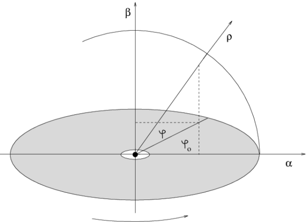
Figure 2: The impact parameters $\alpha,\beta$ in the plane of the sky deduced from the polar coordinates ($\rho,\varphi$). If $\theta_{\mbox{\scriptsize{0}}}$ is the inclination angle of the disk, one have the relation $\tan\varphi_{\mbox{\scriptsize{0}}}=\cos\theta_{\mbox{\scriptsize{0}}}\tan\varphi$

We spot the apparent position of a point P of the disk by its coordinates $(\alpha,\beta)$ in the plane of the sky. A couple $(\alpha,\beta)$ represents the coordinates of the impact parameter of the null geodesic between the disk and the observer. They are measured relative to the direction of the center of the black hole, in the sense of the angular momentum (see Fig. 2). Once again, we use the Carter’s formalism to compute the geodesic between the disk and the observer. We can simply expressed $\lambda$ and $q$ as a function of the impact parameters $\alpha,\beta$ (Cunningham & Bardeen [1973]):

$$\lambda = -\alpha\sin\theta_{0}$$ (40)

$$q = (\beta^{2}-a^{2}\cos^{2}\theta_{0}+\alpha^{2}\cos^{2}\theta_{0})^{1/2}.$$ (41)

Here, $\theta_{0}$ is the inclination angle of the accretion disk. The radius $r_{B}$ of the emitting point of the accretion disk is then calculated by solving the new equation of motion:

$$\int_{\pi/2}^{\theta_{o}}\frac{d\theta}{\sqrt{V_{\theta}}}=\int_{r_{B}}^{\infty}\frac{dr}{\sqrt{V_{r}}}.$$ (42)

Finally, we can expressed the gravitational redshift between a point of the accretion disk and an observer at infinity, needed in Eq. (39), as follows (Cunningham & Bardeen [1973]):

$$(1+z)_{B^{*}\infty}=e^{-\nu}(1-V_{e}^{2})^{-\frac{1}{2}}(1-\Omega_{e}\lambda).$$ (43)

The total spectrum is computed by integrating Eq. (39) over the disk surface. The grid in $(\alpha,\beta)$ is obtained from a elliptic polar coordinates sampling (Fig. 2). The polar angles $\varphi$ are regularly spaced whereas we use a logarithmic sampling of polar radius $\rho$. The Cartesian coordinates ($\alpha,\beta$) are then deduced by the following formulae:

$$\alpha = \rho\cos\varphi$$

$$\beta = \rho\sin\varphi\cos\theta_{0}.$$ (44)

4 Results and Discussion

4.1 The set of parameters

The method described above have been used to obtain spectra emitted by the accretion disk and the hot source. In the Newtonian case, as shown in Paper I, the disk emission depends only on the total luminosity $L_{t}$ and the height $Z_{0}$ of the hot source above the disk. Furthermore, one finds a universal spectrum as a function of a reduced frequency $\nu/\nu_{c}$ and reduced luminosity $\nu F_{\nu}/L_{t}$ where

$$\nu_{c}=\frac{k_{B}}{h}\left(\frac{3L_{t}}{32\pi Z_{0}^{2}\sigma}\right)^{1/4},$$ (45)

corresponding to the characteristic temperature

$$T_{c}=\frac{h}{k_{B}}\nu_{c}.$$ (46)

In the relativistic calculations, one must also specify the mass $M$ and the angular momentum by unit mass $a$ of the black hole. Actually, the disk emission in reduced units depends only on $a$ and $Z_{0}/M$. However, one needs a value of $\nu_{c}$ comparable to the observations, i.e. about $10\,eV$. As an example, for $L_{t}=10^{45}\,erg.s^{-1}$ and $M=5\,10^{6}M_{\sun}$, one gets $\nu_{c}=85\displaystyle\left(\frac{M}{Z_{0}}\right)^{1/2}$eV that is $Z_{0}/M$ about $70$.

The high energy spectrum depends also on the relativistic particle distribution, which was taken as a exponentially cut-off power law (cf. paper I):

$$f(\gamma)\propto\gamma^{-s}\exp(-\frac{\gamma}{\gamma_{0}}).$$ (47)

Thus, one needs also to specify the spectral index $s$, and the cut-off Lorentz factor $\gamma_{0}$ or equivalently the high energy cut-off frequency $\nu_{0}$. Again, the total spectrum is universal for a given value of $a$, $Z_{0}/M$, $\displaystyle\frac{\nu_{0}}{\nu_{c}}$ and $s$. The OSSE/SIGMA observations favor the values $h\nu_{0}\simeq 100\,keV$ and $s\simeq 3$. We have kept these values for all simulations.

4.2 Angular distribution of radiation

As already mentioned, the angular distribution of high energy radiation is entirely determined by the two parameters $\eta_{A}$ and $\chi_{A}$, solutions of the linear system (19). Thus, it depends only on the $G_{n}$’s values, which depend at turn on geometrical factors. Hence, the only relevant parameter is the ratio $Z_{0}/M$. We

Figure 3: Parameters $\eta_{A}$ and $\chi_{A}$ versus $Z_{0}/M$. The Newtonian values without central hole are plotted in solid line and Newtonian values with central hole of radius $1.23M$ (the marginal stability radius corresponding to $a=0.998$) in dashed line. The Kerr values with $a=0.998$ are plotted in dash-dotted line

Figure 4: Polar plots of $\displaystyle\frac{dP}{d\Omega}$ for $Z_{0}/M=100$ (solid line) and $Z_{0}/M=10$ (dashed line). The photon field at the hot source location is less anisotropic as the hot source is closer to the black hole. The bold line corresponds to the Newtonian case

plot in Fig. 3 the curves $\eta_{A}$ and $\chi_{A}$ as a function of $Z_{0}/M$ for $a=0.998$. The differences with the Newtonian case become important for $Z_{0}/M\leq 50$, reaching about $30\%$ at $Z_{0}/M=10$. The closer the source to the black hole is, the smaller $\eta_{A}$ and $\chi_{A}$ are. This corresponds to less anisotropic photon field. This is due to two effects: first the presence of a hole in the accretion disk inside the marginal stability radius; second the curvature of geodesics making the photons emitted near the black hole arrive at larger angle than in the Newtonian case. As shown in Fig. 3, the first effect has a weaker influence than the second one. The polar plot of $\displaystyle\frac{dP}{d\Omega}$ is sketched in Fig. 4 for $Z_{0}=100M$ and $Z_{0}=10M$.

4.3 The radial temperature distribution

We have plotted in Fig. 5 the radial temperature distribution of three models: the Newtonian model of paper I, the

Figure 5: Effective temperature profile of the disk versus r in 3 cases:
a) Our model in Newtonian metrics
b) Our model in Kerr metrics
c) Standard accretion disk
We suppose the same total luminosity in each model

present relativistic model with $a=0.998$ and $Z_{0}/M=70$, and the standard accretion disk model including relativistic effects (Novikov & Thorne [1973]) for the same total luminosity in each cases. The temperature profile is markedly different between the two illumination models and the standard accretion disk one. At large distances, all models give the same asymptotic behavior $T\propto R^{-3/4}$ (cf. paper I). In the inner part of the disk ($R\leq Z_{0}$), in the illumination models, the temperature saturates around the characteristic temperature $T_{c}$. On the other hand, it keeps increasing in the accretion model, where the bulk of the gravitational energy is released at small radii. Thus, for rapidly rotating black hole, the main difference comes from the smaller marginal stability radius ($R_{ms}=1.23\,M$ for $a=0.998$, whereas $R_{ms}=6\,M$ for $a=0$). This increases a lot the accretion efficiency that goes from $\simeq 5.7\%$ for a Schwarzschild black hole ($a=0$), to $\simeq 42\%$ for a maximally rotating Kerr black hole. In the same time the central temperature reaches much higher values. As seen in Fig. 5, these effects have much less influence in the illumination model. Indeed, the power radiated by the disk surface is essentially controlled by $\displaystyle\frac{dP}{d\Omega}$, which is approximately constant for $R\leq Z_{0}$ (i.e. $\theta_{A}\geq\pi/4$) as shown in Fig. 4. So, the differences with the Newtonian model comes only from gravitational and Doppler shifts which are only appreciable for small radii ($R\leq 5M$). Thus, they concern only a small fraction of the emitting area at $T=T_{c}$, unless $Z_{0}$ is itself small enough.

4.4 Overall spectrum

4.4.1 Influence of the hot source’s height

Figure 6: Differential power spectrum for different values of $Z_{0}$ for the Kerr maximal case. We use reduced coordinates

Figure (6) shows the overall spectrum, in reduced units, predicted by the model for different values of $Z_{0}/M$, for $L_{t}=~{}10^{45}\,erg.s^{-1}$, $M=5\,10^{6}\,M_{\sun}$ and $\theta_{0}=0^{\circ}$. The frequency shift at both ends of the spectrum is due to the variations of the characteristic frequency $\nu_{c}$ with $Z_{0}$ (cf. Eq. (45)). The relativistic effects themselves become important for values of $Z_{0}/M$ smaller than about $50$. They produce a variation of intensity lowering the blue-bump and increasing the hard X-ray emission. The change in the UV range is due to the transverse Doppler effect between the rotating disk and the observer, producing a net redshift, the influence of this redshift being more important for small $Z_{0}/M$ as already explained in the last paragraph. In the X-ray range, the variation is due to the change of the parameters $\eta_{A}$ and $\chi_{A}$ when $Z_{0}/M$ decreases (cf. Fig. 3). The observed UV/X ratio can then be strongly altered by these effects. Quantitatively, the ratio between the maximum of the “blue-bump” and the X-ray plateau of our spectra, goes from $\simeq 300$ in the Newtonian case (or, equivalently, for high values of $Z_{0}/M$ in the Kerr metrics), to $\simeq 10$ for $Z_{0}/M=3$ and $\theta_{0}=0^{\circ}$ in the Kerr maximal case, as shown in Fig. 7. This ratio is highly dependent on the inclination angle $\theta_{0}$. By taking the maximum of the“blue-bump” ,which may be not observed, we evidently overestimate the UV/X ratio compared to the observations. It appears also that a small value of

Figure 7: UV/X ratio versus $Z_{0}/M$ for different values of the inclination angle, in the Kerr maximal case.

$Z_{0}/M$ could explain the comparable UV and X-ray fluxes observed in few Seyfert galaxies (Perola et al. [1986], Clavel et al. [1992]). This behavior is clearly the opposite of what we would expect for a hot source whose emission is independent of the disk emission, and thus does not depend on $Z_{0}/M$. In such a case, the smaller the height of the hot source is, the larger the bending effects on the ray of light emitted by the hot source are, increasing the illumination of the disk and thus increasing the UV/X ratio (Martocchia & Matt [1996]). It does not take into account the changes in the hot source emission due to the same bending effects and our model shows that, in this case, the global result is an increase of the X-ray flux toward the observer.

4.4.2 Influence of the inclination angle

Figure 8: Differential power spectrum for different inclination angle, in the Newtonian (solid lines) and the Kerr maximal (dashed lines) cases for $Z_{0}/M=10$. We use reduced coordinates

One can see on Fig. 8 Newtonian and Kerr maximal spectra for different inclination angles for $Z_{0}/M=10$. For small inclination angles, the Kerr spectra are always weaker in UV and brighter in X-ray than the Newtonian ones. However, the difference tends to be less visible for the highest inclination angles. These results can be easily explained: in the X-ray range, as shown in Fig. 4, it is due to the decreasing of the relative difference of the angular distribution between Newtonian and Kerr metrics, as the inclination angle increases. But, for very small values of $Z_{0}/M$, the gravitationnal shift can be so high that the Kerr X-ray spectra appears weaker than the Newtonian one. In the UV band, the relativistic effects (the gravitational shift and the Doppler transverse effect) produce a net redshift in the face-on case ($\theta_{0}=0\degr$) compared to the Newtonian case. For higher inclination angle, the redshifted radiation is compensated by the blueshifted one, coming from the part of the disk moving toward the observer.
These effects are much less pronounced for high $Z_{0}/M$ values because the emission area is much larger, and thus is less affected by relativistic corrections.

5 Conclusion

We have studied the effects of general relativity on the spectrum emitted by our model of re-illumination of the accretion disk of Seyfert I galaxies by a relativistic plasma of leptons. This hot source could be the result of a strong shock between an abortive jet coming from the disk and the interstellar medium. It appears that, by opposition with the standard model of accretion disk including relativistic effects (Sun & Malkan [1989]; Novikov & Thorne [1973]), there are few differences between the Newtonian and relativistic case, unless the height of the hot source is small enough, i.e. $Z_{0}\leq 50M$. Indeed a region of the disk, of length scale of the order of the height $Z_{0}$ of the hot source above the disk (and thus no disturb by the presence of the black-hole for large $Z_{0}$), is equally illuminated and thus predominates in the spectrum.
In a future work, we will study the detailed structure of the hot source, taking into account the microphysical processes like pair production and particle acceleration. As mentioned in paper I, these processes could determine the unknown parameters (upper energy cut-off, spectral index, disk temperature) that are still free in the present theory.

Appendix A Expression of $dS$

The elemental area $dS$ of a parallelogram defined by 2 vectors $\vec{dl_{1}},\ \vec{dl_{2}}$ can be expressed, in curvilinear coordinates, in a general form given by differential geometry. Locally, we can suppose the space to be flat and characterized by 3 vectors $\vec{e_{1}},\ \vec{e_{2}},\ \vec{e_{3}}$. The projections of $dS$ on each plan $(\vec{e_{\alpha}},\vec{e_{\beta}})$ are given by the antisymetrical tensor $dS^{\alpha\beta}$:

$$dS^{\alpha\beta}=dl_{1}^{\alpha}dl_{2}^{\beta}-dl_{1}^{\beta}dl_{2}^{\alpha}$$ (48)

In a 3 space, we rather use the vector $dS_{\alpha}$, dual of $dS_{\alpha\beta}$, defined by:

$$dS_{\alpha}=\frac{1}{2}\sqrt{\gamma}e_{\alpha\beta\gamma}dS^{\beta\gamma}$$ (49)

$\gamma$ is the determinant of the space metric and $e_{\alpha\beta\gamma}$ is the Levi-Civita tensor. We can now obtain the expression of the surface $dS$ modulus of $\vec{dS_{\alpha}}$:

$$dS = \sqrt{dS_{\alpha}dS^{\alpha}}$$ (50)

$$= \sqrt{\gamma^{\alpha\beta}dS_{\alpha}dS_{\beta}}$$ (51)

$$= \sqrt{\gamma\gamma^{\alpha\beta}\frac{1}{2}e_{\alpha\mu\nu}dS^{\mu\nu}\frac{1}{2}e_{\beta\mu^{\prime}\nu^{\prime}}dS^{\mu^{\prime}\nu^{\prime}}}$$ (52)

By setting the 4-tensor $G$ which coefficients are defined by:

$$G_{\mu\nu\mu^{\prime}\nu^{\prime}}=\gamma\gamma^{\alpha\beta}e_{\alpha\mu\nu}e_{\beta\mu^{\prime}\nu^{\prime}}$$ (53)

we can re-write the expression of the elementary surface $dS$ (sum on repeated indices):

$$dS=\sqrt{G_{\mu\nu\mu^{\prime}\nu^{\prime}}dl_{1}^{\mu}dl_{2}^{\nu}dl_{1}^{\mu^{\prime}}dl_{2}^{\nu^{\prime}}}$$ (54)

Appendix B Kerr metric case. Expression of $dS$ in the plan $\theta=0$

In Kerr metric, the space metric tensor is diagonal

$$\gamma_{\alpha\beta} = g_{\alpha\beta}-\frac{g_{0\alpha}g_{0\beta}}{g_{00}}$$ (55)

$$= 0{\ \rm{if\ }}\alpha\neq\beta$$ (56)

To obtain the expression of the elementary surface $dS$ in the plan $\theta=0$ of the disk at radial coordinate $r$, we have to take $\alpha=\beta=\theta$ in Eq. (53). One gets then:

$$dS=\sqrt{\gamma_{rr}\gamma_{\varphi\varphi}}drd\varphi\\$$ (57)

As a matter of interest, the metric coefficients $g_{\alpha\beta}$ we use here, are calculated in the corresponding locally non-rotating frame $\Re$. In the plane $\theta=0$ of the accretion disk, only the $g_{\varphi\varphi}$ metric coefficient differs from the one of Boyer-Lindquist coordinate frame (Eq. (1)). Thus, in frame $\Re$, $\gamma_{rr}$ and $\gamma_{\varphi\varphi}$ are equal to:

$$\left\{\begin{array}[]{lll}\gamma_{rr}&=&\Sigma\Delta^{-1}\\ &&\\ \gamma_{\varphi\varphi}&=&e^{2\psi}\end{array}\right.$$ (58)

A ring surface is obtain after integration of Eq. (57) with respect to $\varphi$, that is:

$$dS=2\pi A^{1/2}\Delta^{-1/2}dr\\$$ (59)

References

- [1972] Bardeen J. M., Press W. H., Teukolsky S. A., 1972, ApJ 178, 347
- [1968] Carter B., 1968, Phys. Rew. 174, 1559
- [1992] Clavel J., Nandra K., Makino F., et al., 1992, ApJ 393, 113
- [1975] Cunningham C. T., 1975, ApJ 202, 788
- [1973] Cunningham C. T., Bardeen J. M., 1973, ApJ 183, 237
- [1991] Ghisellini G., George I. M., Fabian A. C., et al., 1991, MNRAS 248, 14
- [submitted] Henri G., Petrucci P. O., A&A, submitted
- [1996] Martocchia A., Matt G., MNRAS, 282, L53
- [1973] Novikov I. D., Thorne K. S., 1973. In C. DeWitt and B. DeWitt (eds.) Black Holes. Gordon & Breach, New York, p. 343
- [1986] Perola, G. C. , Piro, L. , Altamore, A., et al., 1986, ApJ 306, 508
- [1990] Pounds K. A., Nandra K., Stewart G. C., et al., 1990, Nat 344, 132
- [1984] Rees M, J., 1984, ARA&A 22, 471
- [1973] Shakura N. I., Sunyaev R. A., 1973, A&A 24, 337
- [1989] Sun W-H., Malkan M. A., 1989, ApJ 346, 68