The Evolution of Long-Period Comets

Paul Wiegert

Department of Astronomy

University of Toronto

Toronto, Ontario

M5S 3H8 Canada

and

Scott Tremaine

Canadian Institute for Theoretical Astrophysics

and Canadian Institute for Advanced Research

Program in Cosmology and Gravity

University of Toronto

Toronto, Ontario

M5S 3H8 Canada

Email: tremaine@cita.utoronto.ca

submitted to Icarus, May 1997.

Abstract

We study the evolution of long-period comets by numerical integration of their orbits, a more realistic approach than the Monte Carlo and analytic methods previously used to study this problem. We follow the comets from their origin in the Oort cloud until their final escape or destruction, in a model solar system consisting of the Sun, the four giant planets and the Galactic tide. We also examine the effects of non-gravitational forces and the gravitational forces from a hypothetical solar companion or circumsolar disk. We confirm the conclusion of Oort and other investigators that the observed distribution of long-period comet orbits does not match the expected steady-state distribution unless there is fading or some similar process that depletes the population of older comets. We investigate several simple fading laws. We can match the observed orbit distribution if the fraction of comets remaining observable after $m$ apparitions is $\propto m^{-0.6\pm 0.1}$ (close to the fading law originally proposed by Whipple 1962); or if approximately 95% of comets live for only a few ($\sim 6$) returns and the remainder last indefinitely. Our results also yield statistics such as the expected perihelion distribution, distribution of aphelion directions, frequency of encounters with the giant planets and the rate of production of Halley-type comets.

1 Introduction

Comets can be classified on the basis of their orbital period $P$ into long-period (LP) comets with $P>200{\rm\,yr}$, and short-period (SP) comets with $P<200{\rm\,yr}$; short-period comets are further subdivided into Halley-type comets with $20{\rm\,yr}<P<200{\rm\,yr}$ and Jupiter-family comets with $P<20{\rm\,yr}$ Carusi and Valsecchi (1992). The boundary between SP and LP comets corresponds to a semimajor axis $a=(200)^{2/3}{\rm\,AU}=34.2{\rm\,AU}$, which is useful because: (i) it distinguishes between comets whose aphelia lie within or close to the planetary system, and those that venture beyond; (ii) an orbital period of $200{\rm\,yr}$ corresponds roughly to the length of time over which routine telescopic observations have been taken—the sample of comets with longer periods is much less complete; (iii) the planetary perturbations suffered by comets with periods longer than $200{\rm\,yr}$ are uncorrelated on successive perihelion passages (see footnote 2 below).

LP comets are believed to come from the Oort cloud Oort (1950), a roughly spherical distribution of some $10^{12}$ comets with semimajor axes between $10^{3.5}$ and $10^{4.5}{\rm\,AU}$. The Oort cloud is probably formed from planetesimals ejected from the outer Solar System by planetary perturbations. LP comets—and perhaps some or all Halley-family comets—are Oort-cloud comets that have evolved into more tightly bound orbits under the influence of planetary and other perturbations. Jupiter-family comets probably come from a quite different source, the Kuiper belt outside Neptune, and will not be discussed in this paper.

The observed distribution of the $\sim 700$ known LP comets is determined mainly by celestial mechanics, although physical evolution of the comets (e.g. fading or disruption during perihelion passage near the Sun) and observational selection effects (comets with large perihelion distance are undetectable) also play major roles. The aim of this paper is to construct models of the orbital evolution of LP comets and to compare these models to the observed distribution of orbital elements.

This problem was first examined by Oort (1950), who focused on the distribution of energy or inverse semimajor axis. He found that he could match the observed energy distribution satisfactorily, with two caveats: (i) he had to assume an ad hoc disruption probability $k=0.014$ per perihelion passage; (ii) five times too many comets were present in a spike (the “Oort spike”) near zero energy. Since most of the comets in the Oort spike are on their first passage close to the Sun, he argued that they may contain volatile ices (e.g. CO, CO₂) that create a large bright coma for the new comet, but are substantially or completely depleted in the process. When the comet subsequently returns (assuming it has avoided ejection and other loss mechanisms), it will be much fainter and may escape detection. Most of the decrease in brightness would occur during the first perihelion passage, and the brightness would level off as the most volatile components of the comet’s inventory are lost. This “fading hypothesis” has played a central role in all subsequent attempts to compare the observed and predicted energy distributions of LP comets.

In § 2 we examine the observed distribution of LP comet orbits. The basic theoretical model of LP comet evolution is reviewed in § 3. The simulation algorithm is described in § 4, and the results are presented in § 5. The simulations and results are described in more detail by Wiegert (1996).

2 Observations

The 1993 edition of the Catalogue of Cometary Orbits Marsden and Williams (1993) lists 1392 apparitions of 855 individual comets, of which 681 are LP comets. The catalog includes, where possible, the comet’s osculating orbital elements at or near perihelion. When studying LP comets it is often simpler to work with the elements of the orbit on which the comet approached the planetary system (the “original” elements). These can be calculated from the orbit determined near perihelion by integrating the comet’s trajectory backwards until it is outside the planetary system. Original elements are normally quoted in the frame of the Solar System barycenter. Marsden and Williams list 289 LP comets that have been observed well enough (quality classes 1 and 2) that reliable original elements can be computed.

The difference between the original elements and the elements near perihelion is generally small for the inclination $i$, perihelion distance $q$, argument of perihelion $\omega$ and longitude of the ascending node $\Omega$; when examining the distribution of these elements we will therefore work with the entire sample ($N=681$) of LP comets. The original semimajor axis and eccentricity are generally quite different from the values of these elements near perihelion, so when we examine these elements we shall use only the smaller sample ($N=289$) for which original elements are available.

2.1 Semimajor axis

The energy per unit mass of a small body orbiting a point mass $M_{\odot}$ is $-{\textstyle{1\over 2}}GM_{\odot}/a$, where $a$ is the semimajor axis. This is not precisely the energy per unit mass of a comet orbiting the Sun—the expression neglects contributions from the planets and the Galaxy—but provides a useful measure of a comet’s binding energy. For simplicity, we often use the inverse semimajor axis $x\equiv 1/a$ as a measure of orbital energy. The boundary between SP and LP comets is at $x=(200$ yr$)^{-2/3}=0.029$  AU^-1.

Figure 1 displays histograms of $x=1/a$ for the 289 LP comets with known original orbits, at two different magnifications. The error bars on this and all other histograms are $\pm 1$ standard deviation ($\sigma$) assuming Poisson statistics ($\sigma=N^{1/2}$), unless stated otherwise.

                                $(a)$ $(b)$

                                $(c)$ $(d)$

Figure 1: Distribution of original inverse semimajor axes of 289 LP comets at two different magnifications (panels a,b) and for the 170 LP comets with the most accurate (Class 1) orbits (panels c,d). Data taken from Marsden and Williams (1993). There is no obvious difference between the top and bottom panels, suggesting that observational errors in the inverse semimajor axes are unimportant.

The sharp spike in the distribution for $x\mathrel{\hbox{\hbox to0.0pt{\hbox{\lower 3.0pt\hbox{$\sim$}}\hss}\hbox{\raise 2.0pt\hbox{$<$}}}}10^{-4}{\rm\,AU}^{-1}$ (the “Oort spike”) was interpreted by Oort (1950) as evidence for a population of comets orbiting the Sun at large ($a\mathrel{\hbox{\hbox to0.0pt{\hbox{\lower 3.0pt\hbox{$\sim$}}\hss}\hbox{\raise 2.0pt\hbox{$>$}}}}10~{}000$  AU) distances, a population which has come to be known as the Oort cloud. Comets in the spike are mostly “new” comets, on their first passage into the inner planetary system from the Oort cloud.

                                $(a)$ $(b)$

Figure 2: Number $N$ versus perihelion distance $q$ for 681 LP comets, on two different scales. Data taken from Marsden and Williams (1993). The solid line is the estimated intrinsic distribution from Kresák and Pittich (1978), the dotted line is from Everhart (1967b), and the dashed line is from Shoemaker and Wolfe (1982). The appropriate normalizations are difficult to determine for these curves, and are chosen somewhat arbitrarily.

2.2 Perihelion distance

Figure 2 shows the number of known LP comets versus perihelion distance $q$. The peak near 1  AU is due to observational bias: comets appear brighter when nearer both the Sun and the Earth. The intrinsic distribution $N(q)$ (defined so that $N(q)dq$ is the number of detected and undetected LP comets with perihelion in the interval $[q,q+dq]$) is difficult to determine. Everhart (1967b) concluded that $N(q)\propto 0.4+0.6q$ for $q<1{\rm\,AU}$, and that for $q>1{\rm\,AU}$, $N(q)$ is poorly constrained, probably lying between a flat profile and one increasing linearly with $q$. Kresák and Pittich (1978) also found the intrinsic distribution of $q$ to be largely indeterminate at $q>1$  AU, but preferred a model in which $N(q)\propto q^{1/2}$ over the range $0<q<4$  AU. Shoemaker and Wolfe (1982) estimated $\int_{0}^{q}N(q)dq\propto 500q-175$ for $q>1.3{\rm\,AU}$.

These analyses also yield the completeness of the observed sample as a function of $q$. Everhart estimates that only 20% of observable comets with $q<4$ AU are detected; the corresponding fraction in Shoemaker and Wolfe is 28%. Kresák and Pittich estimate that 60% of comets with $q\leq 1$  AU are detected, dropping to only 2% at $q=4$  AU. Clearly the sample of LP comets is seriously incomplete beyond $q=1$  AU, and the incompleteness is strongly dependent on $q$. In comparing the data to our simulations we must therefore impose a $q$-dependent selection function on our simulated LP comets. We shall generally do this in the crudest possible way, by declaring that our simulated comets are “visible” if and only if $q<q_{\rm v}$, where $q_{\rm v}$ is taken to be 3  AU. This choice is unrealistically large—probably $q_{\rm v}=1.5$  AU would be better—but we find no evidence that other orbital elements are correlated with perihelion distance in the simulations, and the larger cutoff improves our statistics. We shall use the term “apparition” to denote a perihelion passage with $q<q_{\rm v}$.

We have also explored a more elaborate model for selection effects based on work by Everhart (1967a,b; see Wiegert 1996 for details). In this model the probability $p_{\rm v}$ that an apparition is visible is given by

$$p_{\rm v}(q)=\left\{\begin{array}[]{ll}0&\mbox{if $q>2.5$~{}{\rm\,AU}},\\ 2.5-(q/1~{}{\rm\,AU})&\mbox{if $1.5\leq q\leq 2.5$~{}{\rm\,AU}}\\ 1&\mbox{if $q<$ 1.5~{}{\rm\,AU}}\\ \end{array}\right.$$ (1)

The use of this visibility probability in our simulations makes very little change in the distribution of orbital elements (except, of course, for the distribution of perihelion distance). For the sake of brevity we shall mostly discuss simulations using the simpler visibility criterion $q<q_{\rm v}=3{\rm\,AU}$.

2.3 Inclination

Figure 3 shows the distribution of the cosine of the inclination for the LP comets. A spherically symmetric distribution would be flat in this figure, as indicated by the heavy line. Everhart (1967b) argued that inclination-dependent selection effects are minor.

The inclination distribution in ecliptic coordinates is inconsistent with spherical symmetry: the $\chi^{2}$ and Kolmogorov-Smirnov statistics indicate probabilities of only $10^{-4}$ and $10^{-6}$ respectively that the distribution in Fig. 3(a) distribution is flat. Some of the discrepancy may arise from the Kreutz sun-grazer group ($\sim 20$ members), which contributes at $\cos i\sim-0.8$ and $\cos\tilde{\imath}\sim-0.4$. The remaining excess at $|\cos i|\sim 1$ may result from bias towards the ecliptic plane in comet searches, or from an intrinsically anisotropic distribution of LP comets resulting from individual stellar passages through the Oort cloud.

The inclination distribution in Galactic coordinates may have a gap near zero inclination, possibly reflecting the influence of the Galactic tide (§ 4.1.2), or confusion from the dense stellar background in the Galactic plane.

                                $(a)$ $(b)$

Figure 3: The distribution of the cosine of the inclination for the 681 LP comets in (a) ecliptic coordinates, and (b) Galactic coordinates. A spherically symmetric distribution is indicated by the flat line. Data taken from Marsden and Williams (1993).

2.4 Longitude of ascending node

The distribution of longitude of the ascending node $\Omega$ is plotted in Fig. 4. The flat line again indicates a spherically symmetric distribution. The Kreutz sun-grazers are concentrated at $\Omega\sim 0.15$ and $\tilde{\Omega}\sim 4$, and thus are responsible for the highest spike in Fig. 4. Everhart (1967a,b) concluded that $\Omega$-dependent selection effects are likely to be negligible. The $\chi^{2}$ and Kolmogorov-Smirnov statistics indicate that the ecliptic distribution is consistent with a flat distribution at the 80% and 90% levels respectively.

                                $(a)$ $(b)$

Figure 4: The distribution of the longitude of the ascending node of the 681 LP comets in (a) ecliptic coordinates, and (b) Galactic coordinates. Data taken from Marsden and Williams (1993).

2.5 Argument of perihelion

Figure 5 shows the distribution of the argument of perihelion $\omega$ for the LP comets. Comets with $0<\omega<\pi$ outnumber those with $\pi<\omega<2\pi$ by a factor of $395/286=1.38\pm 0.11$. This excess is partly due to the Kreutz group, which is concentrated at $\omega\sim 1.6$ and $\tilde{\omega}\sim 0.15$; but may also be due to observational selection Everhart (1967a); Kresák (1982): comets with $0<\omega<\pi$ pass perihelion above the ecliptic, and are more easily visible to observers in the northern hemisphere. The lack of observed apparitions with $\omega>\pi$ reflects the smaller number of comet searchers in the southern hemisphere until recent times. The distribution in the Galactic frame has a slight excess of comets with orbits in the range $\sin 2\tilde{\omega}>0$ ($399/282=0.59\pm 0.04$).

                                $(a)$ $(b)$

Figure 5: The distribution of the argument of perihelion in $(a)$ the ecliptic frame, $\omega$, and $(b)$ the Galactic frame, $\tilde{\omega}$, for the 681 LP comets. Data taken from Marsden and Williams (1993).

2.6 Aphelion direction

Figure 6 shows the distribution of the aphelion directions of the LP comets in ecliptic and Galactic coordinates.

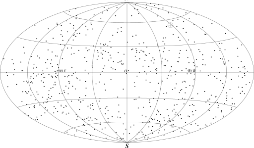
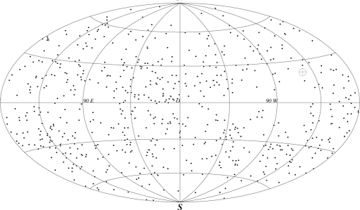
$(a)$ $(b)$

Figure 6: All 681 long-period comet aphelion directions on ecliptic $(a)$ and Galactic $(b)$ equal-area maps. More precisely, these are the antipodes of the perihelion directions. The crossed circle is the solar apex. Data taken from Marsden and Williams (1993).

Claims have been made for a clustering of aphelion directions around the solar antapex (Tyror, 1957; Oja, 1975, e.g. ), but newer analyses with improved catalogues (Lüst, 1984, e.g. ) have cast doubt on this hypothesis. The presence of complex selection effects, such as the uneven coverage of the sky by comet searchers, renders difficult the task of unambiguously determining whether or not clustering is present. Attempts to avoid selection effects end up subdividing the samples into subsamples of such small size as to be of dubious statistical value.

Whipple (1977) has shown that it is unlikely that there are many large comet groups i.e. comets related through having split from the same parent body, in the observed sample though the numerous ($\sim$ 20) observed comet splittings makes the possibility acceptable in principle. A comet group would likely have spread somewhat in semimajor axis: the resulting much larger spread in orbital period $P\propto a^{3/2}$ makes it unlikely that two or more members of such a split group would have passed the Sun in the 200 years for which good observational data exist. The Kreutz group of sun-grazing comets is the only generally accepted exception.

                                $(a)$ $(b)$

Figure 7: The sine of the aphelion latitudes of the 681 LP comets in the ecliptic $(a)$ and Galactic $(b)$ reference frames. The heavy line indicates a spherically symmetric distribution. Data taken from Marsden and Williams (1993).

Figures 7a and b show histograms of comet number versus the sine of the ecliptic latitude $\beta$ and of the Galactic latitude $b$. The ecliptic latitudes deviate only weakly from a spherically symmetric distribution and this deviation is likely due to the lack of southern hemisphere comet searchers. The Galactic distribution shows two broad peaks, centred roughly on $\sin b\sim\pm 0.5$. It will be shown that these probably reflect the influence of the gravitational tidal field of the Galaxy (§ 4.1.2), which acts most strongly when the Sun-comet line makes a $45^{\circ}$ angle with the Galactic polar axis.

2.7 Orbital elements of new comets

For some purposes it is useful to isolate the distribution of orbital elements of the 109 new comets whose original semimajor axes lie in the Oort spike, $x=1/a\leq 10^{-4}\hbox{{\rm\,AU}${}^{-1}$}$. The distributions of perihelion distance, as well as inclination, longitude of the ascending node, and argument of perihelion in Galactic coordinates are all shown in Fig. 8. The distribution of aphelion directions is shown in Fig. 9.

                                $(a)$ $(b)$

                                $(c)$ $(d)$

Figure 8: Distribution of orbital elements for the 109 new comets ($1/a<10^{-4}\hbox{{\rm\,AU}${}^{-1}$}$): (a) perihelion distance; (b) inclination; (c) longitude of ascending node; (d) argument of perihelion. All angular elements are measured in the Galactic frame at the aphelion preceding the first apparition.

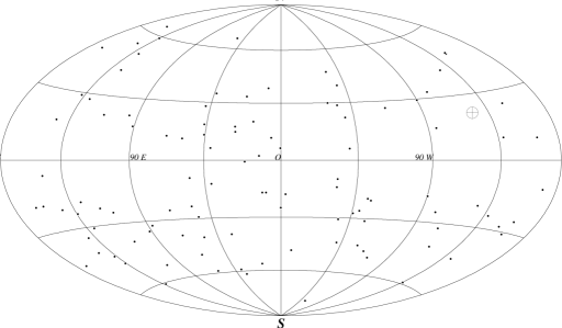
Figure 9: Equal-area plot of the aphelion directions of the 109 new comets in the Galactic frame.

2.8 Parametrization of the distribution of elements

For comparison with theoretical models, we shall parametrize the observed distribution of LP comets by three dimensionless numbers:

• The ratio of the number of comets in the Oort spike ($1/a<10^{-4}\hbox{{\rm\,AU}${}^{-1}$}$) to the total number of LP comets is denoted by $\Psi_{1}$. This parameter measures the relative strength of the Oort spike.

• The inverse semimajor axes of LP comets range from zero (unbound) to 0.029  AU^-1 ($P=200{\rm\,yr}$). Let the ratio of the number of comets in the inner half of this range (0.0145 to 0.029  AU^-1) to the total be $\Psi_{2}$. This parameter measures the prominence of the “tail” of the energy distribution.

• Let the ratio of the number of prograde comets in the ecliptic frame to the total be $\Psi_{3}$. This parameter measures the isotropy of the LP comet distribution.

We estimate these parameters using all LP comets with original orbits in Marsden and Williams (1993):

$$\Psi_{1} = 109/289=0.377\pm 0.042,$$

$$\Psi_{2} = 19/289=0.066\pm 0.016,$$ (2)

$$\Psi_{3} = 145/289=0.501\pm 0.051.$$

For consistency, we based our calculation of $\Psi_{3}$ on the 289 comets with known original orbits, even though knowledge of the original orbit is not required since $\Psi_{3}$ depends only on angular elements. If we consider all 681 LP comets, we find $\Psi_{3}=321/681=0.471\pm 0.041$; the two values are consistent within their error bars.

We denote theoretical values of these parameters by $\Psi_{i}^{t}$ and compare theory and observation through the parameters

$$X_{i}\equiv{\Psi_{i}^{t}\over\Psi_{i}},\qquad i=1,2,3;$$ (3)

which should be unity if theory and observation agree.

3 Theoretical background

3.1 The Oort cloud

The spatial distribution of comets in the Oort cloud can be deduced from the assumption that these comets formed in the outer planetary region and were scattered into the Oort cloud through the combined perturbations of the tide and planets Duncan et al. (1987). These calculations suggest—in order of decreasing reliability—that (i) the cloud is approximately spherical; (ii) the velocity distribution of comets within the cloud is isotropic; in other words the phase-space distribution is uniform on the energy hypersurface, except perhaps at very small angular momentum where the comets are removed by planetary encounters; (iii) the cloud’s inner edge is near 3000  AU, with a space number density of comets roughly proportional to $r^{-3.5}$ from 3000 to 50 000  AU.

Orbits of comets in the Oort cloud evolve mainly due to torques from the overall Galactic tidal field, but they are also affected by encounters with planets, passing stars and molecular clouds. Comets are also lost through collisions with the Sun. Through these mechanisms, between 40% Duncan et al. (1987) and 80% Weissman (1985) of the original Oort cloud may have been lost over the lifetime of the Solar System, leaving perhaps $\sim 10^{12}$ comets (cf. eq. 50) with mass $\sim 50M_{\oplus}$ Weissman (1990) in the present-day comet cloud. These numbers are very uncertain.

If the phase-space distribution of comets is uniform on the energy hypersurface, then the number of comets at a given semimajor axis with angular momentum less than $J$ should be $\propto J^{2}$; this in turn implies that the number of comets with perihelion in the range $[q,q+dq]$ should be $N(q)dq$, where

$$N(q)\propto 1-{q\over a},\qquad q\leq a.$$ (4)

This distribution is modified if there are loss mechanisms that depend strongly on perihelion distance, as we now discuss.

3.2 The loss cylinder

A comet that passes through the planetary system receives a gravitational kick from the planets. The typical energy kick $\Delta x$ depends strongly on perihelion distance (and less strongly on inclination): $\Delta x\approx 1\times 10^{-3}{\rm\,AU}^{-1}$ for $q\mathrel{\hbox{\hbox to0.0pt{\hbox{\lower 3.0pt\hbox{$\sim$}}\hss}\hbox{\raise 2.0pt\hbox{$<$}}}}6{\rm\,AU}$, dropping to $1\times 10^{-4}{\rm\,AU}^{-1}$ at $q\simeq 10{\rm\,AU}$ and $1\times 10^{-5}{\rm\,AU}^{-1}$ at $q\simeq 20{\rm\,AU}$ Fernández (1981); Duncan et al. (1987). For comparison, a typical comet in the Oort spike has $x\mathrel{\hbox{\hbox to0.0pt{\hbox{\lower 3.0pt\hbox{$\sim$}}\hss}\hbox{\raise 2.0pt\hbox{$<$}}}}10^{-4}{\rm\,AU}^{-1}$; since these comets have perihelion $q\sim 1{\rm\,AU}$ they receive an energy kick $\Delta x\gg x$ during perihelion passage. Depending on the sign of the kick, they will either leave the planetary system on an unbound orbit, never to return, or be thrown onto a more tightly bound orbit whose aphelion is much smaller than the size of the Oort cloud. In either case, the comet is lost from the Oort cloud.

More generally, we can define a critical perihelion distance $q_{\ell}\sim 10{\rm\,AU}$ such that comets with $q<q_{\ell}$ suffer a typical energy kick at perihelion which is larger than the typical energy in the Oort cloud. Such comets are said to lie in the “loss cylinder” in phase space because they are lost from the Oort cloud within one orbit (the term “cylinder” is used because at a given location within the cloud, the constraint $q<q_{\ell}$ is is satisfied in a cylindrical region in velocity space: for highly eccentric orbits $q<q_{\ell}$ implies that the angular momentum $J<J_{\ell}\equiv(2GM_{\odot}q_{\ell})^{1/2}$, which in turn implies that the tangential velocity $v_{\perp}<J_{\ell}/r$). The loss cylinder is refilled by torques from the Galactic tide and other sources.

The comets in the Oort spike are inside the loss cylinder and hence must generally be on their first passage through the planetary system (this is why we designated the 109 comets with $1/a<10^{-4}$ AU^-1 as “new” in § 2.7). The loss cylinder concept also explains why the energy spread in the Oort spike is much narrower than the energy spread in the Oort cloud itself: comets with smaller semimajor axes have a smaller moment arm and shorter period so their per-orbit angular momentum and perihelion distance changes are smaller; for $a\mathrel{\hbox{\hbox to0.0pt{\hbox{\lower 3.0pt\hbox{$\sim$}}\hss}\hbox{\raise 2.0pt\hbox{$<$}}}}2\times 10^{4}{\rm\,AU}$ the perihelion cannot jump the “Jupiter barrier” i.e. cannot evolve from $q>q_{\ell}\sim 10{\rm\,AU}$ (large enough to be outside the loss cylinder) to $q\mathrel{\hbox{\hbox to0.0pt{\hbox{\lower 3.0pt\hbox{$\sim$}}\hss}\hbox{\raise 2.0pt\hbox{$<$}}}}1{\rm\,AU}$ (small enough to be visible) in one orbital period. Thus the inner edge of the Oort spike is set by the condition that the typical change in angular momentum per orbit equals the size of the loss cylinder, and does not reflect the actual size of the Oort cloud Hills (1981). The new comets we see come from an outer or active Oort cloud ($a\mathrel{\hbox{\hbox to0.0pt{\hbox{\lower 3.0pt\hbox{$\sim$}}\hss}\hbox{\raise 2.0pt\hbox{$>$}}}}2\times 10^{4}{\rm\,AU}$) in which the typical change in angular momentum per orbit exceeds the size of the loss cylinder. Thus, in the outer Oort cloud, losses from planetary perturbations do not strongly affect the phase-space distribution of comets near zero angular momentum (the loss cylinder is said to be “full”), and the equilibrium distribution of perihelion distances (Eq. 4) remains approximately valid within the loss cylinder. The more massive inner Oort cloud ($a\mathrel{\hbox{\hbox to0.0pt{\hbox{\lower 3.0pt\hbox{$\sim$}}\hss}\hbox{\raise 2.0pt\hbox{$<$}}}}2\times 10^{4}{\rm\,AU}$) does not produce visible comets except during a rare comet “shower” caused by an unusually close stellar encounter and which perturbs them sufficiently to jump the Jupiter barrier. In this inner cloud, losses from planetary perturbations strongly deplete the distribution of comets at small perihelion distances (the loss cylinder is said to be “empty”) and thus it does not contribute to the Oort spike.

3.3 Energy evolution of LP comets

Let us examine the motion of an Oort cloud comet after it enters the planetary system for the first time. The motion of a comet in the field of the giant planets, the Sun and the Galactic tide is quite complicated, but considerable analytic insight can be obtained if we make the following approximations:

1. Depending on the sign of the energy kick from the planets, the comet will either be ejected from the Solar System or perturbed onto a much more tightly bound orbit ($a\sim 10^{3}{\rm\,AU}$). In either case the Galactic tide plays no further significant role, and can be neglected.

2. The influence of the planets is concentrated near perihelion, where the moment arm of the comet is small. Thus the angular momentum, orbit orientation, and perihelion distance are approximately conserved during perihelion passage; the only significant change is in the orbital energy. More precisely, the typical changes in angular elements caused by a planet of mass $M_{p}$ and semimajor axis $a_{p}$ to the orbit of a comet with perihelion $q\mathrel{\hbox{\hbox to0.0pt{\hbox{\lower 3.0pt\hbox{$\sim$}}\hss}\hbox{\raise 2.0pt\hbox{$<$}}}}a_{p}$ are

   $$\Delta i\sim\Delta\Omega\sim\Delta\omega\sim\Delta q/a_{p}\sim M_{p}/M_{\odot},$$ (5)

   while the fractional change in energy is $\Delta x/x\sim(aM_{p}/a_{p}M_{\odot})$, which is much larger for an Oort cloud comet (by a factor $a/a_{p}\sim 10^{3}$–$10^{4}$).

3. The orbit of any LP comet looks nearly parabolic when it passes through the planetary system, so the distribution of energy changes during perihelion passage is approximately independent of the comet’s orbital energy. Therefore we may define a function $p(\Delta x)d\Delta x$, the probability that the energy change per perihelion passage due to planetary perturbations is in the interval $[\Delta x,\Delta x+d\Delta x]$. The function $p(\Delta x)$ is an implicit function of the inclination, perihelion distance, argument of perihelion, etc. but as we have seen these change much more slowly than $x$ and so can be considered constants. The properties of $p(\Delta x)$ are discussed by Everhart (1968); $p$ is approximately an even function of $\Delta x$ [the odd component is smaller by O$(M_{p}/M_{\odot})$] and as $|\Delta x|\to\infty$, $p(\Delta x)\propto|\Delta x|^{-3}$—although despite this extended tail $p$ is often approximated by a Gaussian. If $q\mathrel{\hbox{\hbox to0.0pt{\hbox{\lower 3.0pt\hbox{$\sim$}}\hss}\hbox{\raise 2.0pt\hbox{$<$}}}}a_{p}$ then the typical energy change due to a single planet is $\langle|\Delta x|\rangle\sim(M_{p}/M_{\odot})a_{p}^{-1}$. Plots of the second moment of $p(\Delta x)$, averaged over argument of perihelion, as a function of perihelion distance and inclination are given by Fernández (1981) and Duncan et al. (1987).

4. Comets on escape orbits ($x\leq 0$) are lost from the Solar System. The appropriate boundary condition at large $x$ is less clear. Our other approximations fail when $x$ becomes comparable to the inverse semimajor axes of the planets, which occurs when they become SP comets at $x=x_{\rm sp}=0.029{\rm\,AU}^{-1}$. SP comets will continue to random walk in energy—some becoming LP comets once again—but the other orbital elements will also evolve at a comparable rate, so the approximation of a one-dimensional random walk is no longer valid. Fortunately we shall find that the fraction of new comets that survive fading and ejection to become SP comets is small enough that the details of their evolution are unlikely to affect the overall distribution of LP comets (cf. Tables I and III); for most purposes we can simply assume that LP comets reaching $x_{\rm sp}$ are lost.

5. The orbital periods of most LP comets are sufficiently long that the orbital phases of the planets and hence the energy kicks that the comet receives from them are uncorrelated at successive encounters. Thus the evolution of the comet energy can be regarded as a Markov process or random walk.

6. A comet may fade as its inventory of volatiles is depleted or may be disrupted by various mechanisms. We shall use the term “fading” to denote any change in the intrinsic properties of the comet that would cause it to disappear from the observed sample. We parametrize this process by a function $\Phi_{m}\in[0,1]$, $m=1,2,\ldots$ ($\Phi_{1}=1$), the probability that a visible new comet survives fading for at least $m$ perihelion passages. There are two closely related functions: the probability that the comet survives fading for precisely $m$ perihelion passages,

   $$\phi_{m}\equiv\Phi_{m}-\Phi_{m+1};$$ (9)

   and the conditional probability that a comet that survives $m$ passages will fade before the $(m+1)^{\rm st}$ passage,

   $$\psi_{m}={\phi_{m}\over\Phi_{m}}=1-{\Phi_{m+1}\over\Phi_{m}}.$$ (10)

With these approximations the evolution of the energy of LP comets can be treated as a one-dimensional random walk. We assume that visible new comets arrive directly from the Oort cloud with original energy $x=0$, at a rate $N$ per year. Let $f_{m}(x)dx$ be the number of visible LP comets per year with original energy in the range $[x,x+dx]$ which are returning on their $m^{\rm th}$ perihelion passage (thus $f_{1}(x)=N\delta(x)$, where $\delta(x)$ is a delta function). Then in a steady state we must have

$$f_{m+1}(x)=(1-\psi_{m})\int_{0}^{\infty}f_{m}(y)p(x-y)dy,\quad m\geq 1,\ x\geq 0,$$ (11)

which can be solved successively for $f_{2}(x),f_{3}(x),\ldots$. The total number of LP comets with energies in the interval $[x,x+dx]$ is $f(x)dx$, where $f(x)=\sum_{m=0}^{\infty}f_{m}(x)$; theoretical predictions of $f(x)$ are to be compared with the observed distribution of LP comets in Fig. 1.

The simplest version of this problem is obtained by assuming that there is no fading ($\psi_{m}=0$) and that the energy changes by discrete steps $\pm\epsilon$ with equal probability [$p(x)={\textstyle{1\over 2}}\delta(x+\epsilon)+{\textstyle{1\over 2}}\delta(x-\epsilon)$]. In this case the possible values of the energy are restricted to a lattice $x=(j-1)\epsilon$, where $j$ is an integer, and the random walk is identical to the gambler’s ruin problem Kannan (1979); Feller (1968). The end-state of ejection ($j=0$) corresponds to bankruptcy; if in addition we assume that there is an absorbing boundary at $x_{\rm sp}\equiv(j_{\rm sp}-1)\epsilon$, then evolving to an SP comet corresponds to breaking the house. Thus, for example, the probabilities that an LP comet with energy $(j-1)\epsilon$ will be eventually be ejected or become a short-period comet are respectively

$$p_{\rm ej}=1-{j\over j_{\rm sp}},\qquad p_{\rm sp}={j\over j_{\rm sp}},$$ (12)

and the mean number of orbits that the comet will survive is

$$\langle m\rangle=j(j_{\rm sp}-j).$$ (13)

A new comet has $j=1$ and its mean lifetime is therefore $\langle m\rangle=j_{\rm sp}-1$; the ratio of new to all LP comets observed in a fixed time interval is

$$\Psi_{1}^{t}={1\over\langle m\rangle}={1\over j_{\rm sp}-1}.$$ (14)

There are also explicit expressions for the probability that the comet is ejected or becomes an SP comet at the $m^{\rm th}$ perihelion passage Feller (1968).

The gambler’s ruin problem is particularly simple if there is no boundary condition at large $x$ ($x_{\rm sp}\to\infty$), which is reasonable since few comets reach short-period orbits anyway (§ 5.2.1). The probability that a new comet will survive for precisely $m$ orbits is then

$$p_{\rm ej}(m) = {1\over 2^{m}m}\left(m\atop{\textstyle{1\over 2}}m+{\textstyle{1\over 2}}\right),\quad\hbox{$m$ odd},$$ (15)

$$= 0\qquad\qquad\hbox{$m$ even};$$

for $m\gg 1$, $p_{\rm ej}(m)\to(2/\pi)^{1/2}m^{-3/2}$ for $m$ odd, and zero otherwise. The mean lifetime $\sum_{m=1}^{\infty}mp_{\rm ej}(m)$ is infinite, and the probability that a comet will survive for at least $m$ orbits is $\sim m^{-1/2}$ for large $m$.

When using the gambler’s ruin to model the evolution of LP comets, we take $\epsilon\simeq 5\times 10^{-4}\hbox{{\rm\,AU}${}^{-1}$}$, which is the rms energy change for comets with perihelion between 5 and $10{\rm\,AU}$ Fernández (1981); Duncan et al. (1987), and $x_{\rm sp}=0.029\hbox{{\rm\,AU}${}^{-1}$}$ ($P=200{\rm\,yr}$); thus $j_{\rm sp}\simeq 60$. Eq. 14 then predicts $\Psi_{1}^{t}=0.017$; the ratio of the predicted to the observed value for this parameter (cf. Eq. 2.8) is

$$X_{1}={\Psi_{1}^{t}\over\Psi_{1}}=0.051\pm 0.006.$$ (16)

The gambler’s ruin model predicts far too few comets in the Oort spike relative to the total number of LP comets.

This simple model also makes useful predictions about the inclination distribution of LP comets. The distribution of new comets is approximately isotropic, so there are equal numbers of prograde and retrograde new comets. Since prograde comets have longer encounter times with the planets, they tend to have larger energy changes than retrograde comets. Equation 14 predicts that the ratio of prograde to retrograde LP comets should be roughly the ratio of the rms energy change for these two types, $\epsilon_{\rm retro}/\epsilon_{\rm pro}\simeq$2–3. The fraction of prograde comets should then be $\Psi_{3}^{t}=1/(1+\epsilon_{\rm pro}/\epsilon_{\rm retro})\simeq 0.3$. The ratio of the predicted to the observed value for this parameter (cf. Eq. 2.8) is

$$X_{3}={\Psi_{3}^{t}\over\Psi_{3}}=0.58\pm 0.06.$$ (17)

The gambler’s ruin model predicts too few prograde comets.

More accurate investigations of this one-dimensional random walk have been carried out by many authors. Oort (1950) approximated $p(\Delta x)$ by a Gaussian and assumed $\psi_{m}=k=\hbox{constant}$ and found a good fit to most of the energy distribution for $k=0.014$; however, he found that the number of new comets was larger than the model predicted by a factor of five, and hence was forced to assume that only one in five new comets survive to the second perihelion passage—in other words $\psi_{1}=0.8$, $\psi_{m}=0.014$ for $m>1$. Kendall (1961) and Yabushita (1979) have analyzed the case $x_{\rm sp}\to\infty$, $\psi_{m}=k=\hbox{constant}$, $p(y)\propto\exp\left(-2^{1/2}|y|/\sigma\right)$, where $\sigma$ is the rms energy change per perihelion passage. In this case Eq. 11 can be solved analytically to yield

$$f(x)=N\delta(x)+{2^{1/2}N\over\sigma}\big{(}1-k^{1/2}\big{)}\exp\big{[}-(2k)^{1/2}x/\sigma\big{]};$$ (18)

using this result Kendall derives a reasonable fit to the data if $k=0.04$ and one in four to six new comets survive to the second perihelion—results roughly compatible with Oort’s. This model predicts a ratio of new comets to all LP comets observed in a fixed time interval given by

$$\Psi_{1}^{t}={N\over\int f(x)dx}=k^{1/2}.$$ (19)

Yabushita (1979) gave analytic formulae for $p_{\rm ej}(m)$ for this model, and showed that the probability that a comet will survive for at least $m$ orbits is $\sim\exp(-km)/m^{1/2}$ for large $m$. Whipple (1962) examined survival laws of the form $\phi_{m}\propto m^{-\alpha}$ (the proportionality constant is determined by the condition that $\sum_{m}\phi_{m}=1$) and found a good fit to the observed energy distribution with $\alpha\simeq 1.7$. Everhart (1979) used a distribution $p(y)$ derived from his numerical experiments and found $\Phi_{m}\simeq 0.2$ for all $m>1$; in other words only one in five comets survived to the second perihelion passage but the fading after that time was negligible.

For some purposes the random walk can be approximated as a diffusion process; in this case the relevant equations and their solutions are discussed by Yabushita (1980). Bailey (1984) examines solutions of a diffusion equation in two dimensions (energy and angular momentum) and includes a fading probability that depends on energy rather than perihelion number—which is less well-motivated but makes the equations easier to solve (he justifies his fading function with an a posteriori “thermal shock” model, in which comets with large aphelia are more susceptible to disruption because they approach perihelion with a lower temperature). Bailey finds a good fit to the observed energy distribution if the fading probability per orbit is

$$\phi(x)=0.3[1+(x/0.004{\rm\,AU})^{2}]^{-3/2}.$$ (20)

Emel’yanenko and Bailey (1996) have modeled the distribution of LP comets using a Monte Carlo model with $\psi_{m}=k=\hbox{constant}$ plus an additional probability per orbit $k^{\ast}$ that the comet is rejuvenated. Their preferred values are $k=0.3$ and $k^{\ast}=0.0005$.

The most complete model of LP comet evolution based on a random walk in energy is due to Weissman (1978, 1979, 1980). His Monte Carlo model included the gravitational influence of the planets, non-gravitational forces, forces from passing stars, tidal disruption by the Sun, fading and splitting. In his preferred model, 15% of the comets have zero fading probability, and the rest had a fading probability of 0.1 per orbit. At this cost of this somewhat ad hoc assumption, Weissman was able to successfully reproduce the semimajor axis, inclination, and perihelion distributions.

The one-dimensional random walk is a valuable tool for understanding the distribution of LP comets. However, some of its assumptions are not well-justified: (i) Secular changes in perihelion distance, argument of perihelion, and inclination at each perihelion passage accumulate over many orbits and can lead to substantial evolution of the orientation and perihelion Quinn et al. (1990); Bailey et al. (1992); Thomas and Morbidelli (1996). (ii) Although the probability distribution of energy changes $p(y)$ is approximately an even function [$\langle y^{2}\rangle^{1/2}$ is larger than $\langle y\rangle$ by O$(M_{p}/M_{\odot})$], the random changes in energy due to the second moment grow only as $m^{1/2}$ where $m$ is the number of orbits, while the systematic changes due to the first moment grow as $m$. Thus the small asymmetry in $p(y)$ may have important consequences.

3.4 The fading problem

All the investigations described in the previous subsection reach the same conclusion: if the LP comets are in a steady state then we cannot match the observed energy distribution without unexpectedly strong fading after the first perihelion passage. Therefore either (i) the comet distribution is not in a steady state, which almost certainly requires rejecting most of the Oort model, or (ii) we must postulate ad hoc fading laws and abandon the use of the energy distribution as a convincing test of the Oort model. This is the fading problem.

Fading can arise from many possible mechanisms but the most natural hypothesis is that the comet’s brightness fades sharply because its inventory of volatiles is depleted during the first perihelion passage. Oort and Schmidt (1951) have argued that this hypothesis is supported by the observation that new comets have strong continuum spectra due to dust entrained by the gases from a volatile component, and that the decline of brightness with increasing heliocentric distance is much slower for new comets. Many authors have looked for evidence that new comets differ in composition or brightness from older LP comets, with mixed results; Whipple (1991) summarizes these investigations by saying that the Oort-Schmidt effect is “fairly well confirmed”.

Fading is much slower after the first perihelion passage, as exemplified by the long history of Halley’s comet. Whipple (1992) concludes that there is no strong evidence that older (i.e. shorter period) LP comets have faded relative to younger LP comets, consistent with theoretical estimates that $10^{3}$–$10^{4}$ orbits are required for moderate-sized comets to lose their volatiles Weissman (1980) and the lack of strong systematic trends in the brightness of SP comets.

Comets may also fade if they disrupt or split. After splitting, the fragments are fainter and hence less likely to be visible, and in addition lose their volatiles more rapidly. Moreover, young comets are more likely to split than old ones: Weissman (1980) gives splitting probabilities per perihelion passage of $0.10\pm 0.04$ for new comets but only $0.045\pm 0.011$ for LP comets in general. The cause of splitting is not well understood, except in some cases where splitting is due to tidal forces from a close encounter with a giant planet.

Finally, we note that LP comets are responsible for 10–30% of the crater production by impact on Earth Shoemaker (1983). The observed cratering rate can therefore—in principle—constrain the total population of LP comets, whether or not they have faded; however, this constraint is difficult to evaluate, in part because estimates of comet masses are quite uncertain.

4 Algorithm

We represent each comet by a massless test particle and neglect interactions between comets. The orbit of the test particle is followed in the combined gravitational fields of the Sun, the four giant planets, and the Galactic tide. We assume that the planets travel around the Sun in circular, coplanar orbits. We neglect the terrestrial planets, Pluto, the small free inclinations and eccentricities of the giant planets, and their mutual perturbations as there is no reason to expect that these play significant roles in the evolution of LP comets.

4.1 Equations of motion

The equation of motion of the comet can be written as

$$\!\!\!\!\!\!\!\!\!\!\ddot{{\bf r}}={\bf F}_{\odot}+{\bf F}_{\rm planets}+{\bf F}_{\rm tide}+{\bf F}_{\rm other},$$ (21)

where the terms on the right side represent the force per unit mass from the Sun, the planets, the Galactic tide, and other sources (e.g. non-gravitational forces).

4.1.1 The planets

We shall employ two frames of reference: the barycentric frame, whose origin is the center of mass of the Sun and the four planets, and the heliocentric frame, whose origin is the Sun. In the barycentric frame,

$${\bf F}_{\odot}+{\bf F}_{\rm planets}=-\frac{GM_{\odot}}{|{\bf r}-{\bf r}_{\odot}|^{3}}({\bf r}-{\bf r}_{\odot})-\sum\limits_{p}\frac{GM_{p}}{|{\bf r}-{\bf r}_{p}|^{3}}({\bf r}-{\bf r}_{p}),$$ (22)

where ${\bf r}$, ${\bf r}_{\odot}$, and ${\bf r}_{p}$ are the positions of the comet, the Sun, and planet $p$. In the heliocentric frame, the Sun is at the origin and

$${\bf F}_{\odot}+{\bf F}_{\rm planets}=-\frac{GM_{\odot}}{|{\bf r}|^{3}}{\bf r}-\sum\limits_{p}\frac{GM_{p}}{|{\bf r}-{\bf r}_{p}|^{3}}({\bf r}-{\bf r}_{p})-\sum\limits_{p}\frac{GM_{p}}{|{\bf r}_{p}|^{3}}{\bf r}_{p};$$ (23)

the last sum is the “indirect term” that arises because the heliocentric frame is not inertial.

The heliocentric frame is useful for integrating orbits at small radii, $|{\bf r}|\mathrel{\hbox{\hbox to0.0pt{\hbox{\lower 3.0pt\hbox{$\sim$}}\hss}\hbox{\raise 2.0pt\hbox{$<$}}}}|{\bf r}_{p}|$, because it ensures that the primary force center, the Sun, is precisely at the origin (see §4.1.4). It is not well-suited for integrating orbits at large radii, $|{\bf r}|\mathrel{\hbox{\hbox to0.0pt{\hbox{\lower 3.0pt\hbox{$\sim$}}\hss}\hbox{\raise 2.0pt\hbox{$>$}}}}|{\bf r}_{p}|$, because the indirect term does not approach zero at large radii, and oscillates with a period equal to the planetary orbital period—thereby forcing the integrator to use a very small timestep. In the integrations we switch from heliocentric to barycentric coordinates when the comet radius $|{\bf r}|$ exceeds a transition radius $r_{c}$; tests show that the integrations are most efficient when $r_{c}=10{\rm\,AU}$.

The code tracks close encounters and collisions between comets and planets. A close encounter with a planet is defined to be a passage through a planet’s sphere of influence

$$R_{\scriptscriptstyle I}=\left(\frac{M_{p}}{M_{\odot}}\right)^{2/5}a_{p},$$ (24)

where $a_{p}$ is the planet’s semimajor axis. Each inward crossing of the sphere of influence is counted as one encounter, even if there are multiple pericenter passages while the comet remains within the sphere of influence. A close encounter with the Sun is defined to be a passage within 10 solar radii.

4.1.2 The Galactic tide

The effects of the Galactic tide on comet orbits are discussed by Heisler and Tremaine (1986), Morris and Muller (1986), Torbett (1986), and Matese and Whitman (1989). Consider a rotating set of orthonormal vectors $\{{\bf e}_{\tilde{x}},{\bf e}_{\tilde{y}},{\bf e}_{\tilde{z}}\}$. Let ${\bf e}_{\tilde{x}}$ point away from the Galactic center, ${\bf e}_{\tilde{y}}$ in the direction of Galactic rotation, and ${\bf e}_{\tilde{z}}$ towards the South Galactic Pole (South is chosen so that the coordinate system is right-handed). The force per unit mass from the tide is Heisler and Tremaine (1986)

$$\!\!\!\!\!\!\!\!\!\!{\bf F}_{\rm tide}=(A-B)(3A+B)\tilde{x}{\bf e}_{\tilde{x}}-(A-B)^{2}\tilde{y}{\bf e}_{\tilde{y}}-[4\pi G\rho_{0}-2(B^{2}-A^{2})]\tilde{z}{\bf e}_{\tilde{z}},$$ (25)

where $\rho_{0}$ is the mass density in the solar neighborhood, and $A$ and $B$ are the Oort constants. We take $A=14.4\pm 1.2$ km s${}^{-1}~{}$kpc^-1 and $B=-12.0\pm 2.8$ km s^-1 kpc^-1 Kerr and Lynden-Bell (1986). The local mass density is less well-known. Visible matter (stars and gas) contributes about $0.1$ M_⊙ pc^-3, but the amount of dark matter present in the solar neighbourhood remains controversial. If the dark matter is distributed like the visible matter, then the dark/visible mass ratio $P$ is between 0 and 2 Oort (1960); Bahcall (1984); Kuijken and Gilmore (1989); Kuijken (1991); Bahcall et al. (1992). We adopt $\rho_{0}=0.15$ M_⊙  pc^-3 in this paper, corresponding to $P=0.5$.

With these values of $A$, $B$ and $\rho_{0}$, the $4\pi G\rho_{0}$ term of Eq. 25 exceeds the others by more than a factor of ten, and from now on we shall neglect these other terms. The dominant component of the tidal force arises from a gravitational potential of the form

$$V_{\rm tide}=2\pi G\rho_{0}\tilde{z}^{2}.$$ (26)

In practice, of course, the local density $\rho_{0}$ varies as the Sun travels up and down, in and out, and through spiral arms during its orbit around the Galaxy. The amplitude of this variation depends strongly on the unknown distribution and total amount of disk dark matter. The maximum-to-minimum density variation could be as large as 3:1 Matese et al. (1995) but is probably considerably smaller, with a period around 30 Myr [close to ${\textstyle{1\over 2}}(\pi/G\rho_{0})^{1/2}$, the half-period for oscillations in the potential (26) ]. We are justified in neglecting these variations in $\rho_{0}$, because the typical lifetime of LP comets after their first apparition is only 1.4 Myr (see Table III below), which is much shorter.

4.1.3 Encounters with stars and molecular clouds

Our model neglects the effects of passing stars on LP comets, for two main reasons: (i) The delivery rate of Oort cloud comets to the planetary system due to Galactic tides is higher than the rate due to stellar encounters by a factor 1.5–2 Heisler and Tremaine (1986); Torbett (1986), except during rare comet showers caused by an unusually close passage, during which the delivery rate may be enhanced by a factor of twenty or so Hills (1981); Heisler (1990); we feel justified in neglecting the possibility of a comet shower because they only last about 2% of the time Heisler (1990); (ii) The effects of stellar encounters are highly time-variable whereas the strength of the tide is approximately constant over the typical lifetime of LP comets; thus by concentrating on the effects of the tide we focus on a deterministic problem, whose results are easier to interpret.

The effects of rare encounters with molecular clouds are highly time-variable, and difficult to estimate reliably because the properties of molecular clouds are poorly known Bailey (1983); Drapatz and Zinnecker (1984); Hut and Tremaine (1985); Torbett (1986). Therefore we shall also assume that the present distribution of LP comets has not been affected by a recent encounter with a molecular cloud.

4.1.4 Regularisation

Integrating the orbits of LP comets is a challenging numerical problem, because of the wide range of timescales (the orbital period can be several Myr but perihelion passage occurs over a timescale as short as months) and because it is important to avoid any secular drift in energy or angular momentum due to numerical errors. We have used the Kustaanheimo–Stiefel (K-S) transformation to convert Cartesian coordinates to regularized coordinates and have carried out all of our integrations in the regularized coordinates. A requirement of K–S regularisation is that the frame origin must coincide with the primary force centre, which is why we use heliocentric coordinates at small radii.

The numerical integrations were carried out using the Bulirsch-Stoer method, which was checked using a fourth-order Runge-Kutta-Fehlberg algorithm. All integrations were done in double-precision arithmetic.

4.2 Non-gravitational forces

The asymmetric sublimation of cometary volatiles results in a net acceleration of the nucleus. These non-gravitational (NG) forces are limited to times of significant outgassing (i.e. coma production), and remain small even then.

Non-gravitational forces are difficult to model. Their strength obviously depends on the comet’s distance from the Sun, but displays less regular variability as well: gas production may vary by a factor of 2 or more between the pre- and post-perihelion legs of the orbit Sekanina (1964); Festou (1986), and jets and streamers are observed to evolve on time scales of less than a day Festou et al. (1993b), suggesting that NG forces change on similar time scales. Further complications arise from the rotation of the nucleus, which is difficult to measure through the coma, and which may be complicated by precession Wilhelm (1987).

The NG acceleration ${\bf F}_{\rm jet}$ is written as

$${\bf F}_{\rm jet}=F_{1}{\bf e}_{1}+F_{2}{\bf e}_{2}+F_{3}{\bf e}_{3},$$ (27)

where ${\bf e}_{1}$ points radially outward from the Sun, ${\bf e}_{2}$ lies in the orbital plane, pointing in the direction of orbital motion and normal to ${\bf e}_{1}$, and ${\bf e}_{3}={\bf e}_{1}\times{\bf e}_{2}$. A naive model of NG accelerations, which is all the data allows, assumes that the short timescale components are uncorrelated and cancel out, leaving only fairly regular, longer timescale components as dynamically important. We shall use the Style II model of Marsden et al. (1973), which assumes that accelerations are symmetric about perihelion, and can be represented by

$$F_{1}(r)=A_{1}g(r),\hskip 28.45274ptF_{2}(r)=A_{2}g(r),\hskip 28.45274ptF_{3}(r)=A_{3}g(r).$$ (28)

Here $\{A_{1},A_{2},A_{3}\}$ are independent constants, and $g(r)$ is a non-negative function describing the dependence on the comet-Sun distance $r$. The form of $g(r)$ is based on an empirical water sublimation curve by Delsemme and Miller (1971),

$$g(r)=\alpha\left(\frac{r}{r_{0}}\right)^{-m}\left[1+\left(\frac{r}{r_{0}}\right)^{n}\right]^{-k},$$ (29)

where $m=2.15$, $k=4.6142$, $n=5.093$, $r_{0}=2.808$  AU and $\alpha$ is chosen to be 0.1113 so that $g(1~{}$ AU$)=1$. Note that $g(r)$ is roughly proportional to $r^{-m}\approx r^{-2}$ for $r\ll r_{0}$. At $r\gg r_{0}$, $g(r)$ drops much faster than the simple inverse square that describes the incident solar flux.

The constants $A_{i}$ are determined by fitting individual comet orbits Marsden et al. (1973); the value of $A_{1}$ is typically $10^{-7}$ to $10^{-9}$  AU day^-2, $|A_{2}|$ is typically only 10% of $|A_{1}|$, and $A_{3}$ is consistent with zero.

4.3 Initial conditions

4.3.1 Initial phase-space distribution

The distribution of comets in the Oort cloud is only poorly known, although it is plausible to assume that the cloud is roughly spherical and that the comets are uniformly distributed on the energy hypersurface in phase space, except possibly at very small angular momenta (cf. §3.1). Then the phase-space density is a function only of $L\equiv(GM_{\odot}a)^{1/2}$, which we assume to be

$$f(L)=\left\{\begin{array}[]{cc}0,&L<L_{-}=(GM_{\odot}a_{-})^{1/2},\\ f_{0}L^{2\alpha+3},&L_{-}\leq L\leq L_{+},\\ 0,&L>L_{+}=(GM_{\odot}a_{+})^{1/2},\end{array}\right.$$ (30)

where $f_{0}$ and $\alpha$ are constants, and $a_{-}$ and $a_{+}$ are the inner and outer edges of the Oort cloud, respectively. We show below (footnote 7) that the total number of Oort cloud comets with semimajor axes in the range specified by $[L,L+dL]$ is $(2\pi)^{3}f(L)L^{2}dL$; this in turn implies that the number density of comets is $\propto r^{\alpha}$ for $a_{-}\ll r\ll a_{+}$.

Simulations of the formation of the Oort cloud by Duncan et al. (1987) suggest that the number density of Oort cloud comets is $\propto r^{-(3.5\pm 0.5)}$ between 3000 and 50 000  AU. Thus we set $\alpha=-3.5$, $a_{-}=10~{}000~{}{\rm\,AU}$ and $a_{+}=50~{}000$  AU. The inner edge of the cloud was placed at  10 000  AU instead of 3000  AU because comets with $a<10~{}000{\rm\,AU}$ cannot become visible except in occasional comet showers, yet would consume most of the computer time in our simulation.

If the comets are uniformly distributed on the energy hypersurface, the fraction of cloud comets with perihelion less than $q\ll a$ is $J^{2}(q)/L^{2}=2q/a=0.003(q/40{\rm\,AU})(25,000{\rm\,AU}/a)$ (which is consistent with $\int N(q)dq$ as given by Eq. 4). Since the effects of the planets decline rapidly to zero when $q\mathrel{\hbox{\hbox to0.0pt{\hbox{\lower 3.0pt\hbox{$\sim$}}\hss}\hbox{\raise 2.0pt\hbox{$>$}}}}40{\rm\,AU}$, only a small fraction of cloud comets are influenced by planetary perturbations. Therefore to avoid wasting computer time we analyze the motion of comets with larger perihelion distance analytically, as we now describe.

4.3.2 Orbit-averaged evolution

For comets in the Oort cloud, the tidal potential (26) is much smaller than the Kepler Hamiltonian $H_{\rm Kep}=-{\textstyle{1\over 2}}GM_{\odot}/a$. Thus the evolution of the comet under the Hamiltonian $H_{\rm Kep}+V_{\rm tide}$ can be approximately described by averaging $V_{\rm tide}$ over one period of a Kepler orbit to obtain the orbit-averaged Hamiltonian Heisler and Tremaine (1986)

$$H_{\rm av}=-\frac{GM_{\odot}}{2a}+\pi G\rho_{0}\,a^{2}\sin^{2}\!\tilde{\imath}\>(1-e^{2}+5e^{2}\sin^{2}\tilde{\omega});$$ (31)

here $\tilde{\imath}$ and $\tilde{\omega}$ are the inclination and argument of perihelion measured in the Galactic frame. It is useful to introduce canonical momenta

$$L\equiv(GM_{\odot}a)^{1/2},\quad J=[GM_{\odot}a(1-e^{2})]^{1/2},\quad J_{\tilde{z}}=J\cos\tilde{\imath}$$ (32)

and their conjugate coordinates

$$f,\qquad\tilde{\omega},\qquad\tilde{\Omega}.$$ (33)

Here $J$ is the usual angular momentum per unit mass, $J_{\tilde{z}}$ is its component normal to the Galactic plane, $f$ is the true anomaly and $\tilde{\Omega}$ is the longitude of the ascending node on the Galactic plane. In terms of the canonical coordinates and momenta the orbit-averaged Hamiltonian is

$$H_{\rm av}=-\frac{(GM_{\odot})^{2}}{2L^{2}}+\frac{\pi\rho_{0}}{GM_{\odot}^{2}}\frac{L^{2}}{J^{2}}(J^{2}-J_{\tilde{z}}^{2})\left[J^{2}+5(L^{2}-J^{2})\sin^{2}\tilde{\omega}\right].$$ (34)

The canonical variables $f$ and $\tilde{\Omega}$ are absent from Eq. 34, so the conjugate momenta $L$ and $J_{\tilde{z}}$ are conserved. The conservation of $L$ implies that semimajor axis is conserved as well. The solution of the equations of motion (34) is discussed by Heisler and Tremaine (1986) and Matese and Whitman (1989) but is not needed for our purposes.

The rate of change of angular momentum is given by

$$\dot{J} = -\frac{\partial H_{\rm av}}{\partial\tilde{\omega}},$$ (35)

$$= -\frac{5\pi\rho_{0}}{GM_{\odot}^{2}}\frac{L^{2}}{J^{2}}\>(J^{2}-J_{\tilde{z}}^{2})(L^{2}-J^{2})\>\sin 2\tilde{\omega},$$ (36)

$$= -\frac{5\pi\rho_{0}}{GM_{\odot}^{2}}e^{2}L^{4}\sin^{2}\tilde{\imath}\sin 2\tilde{\omega},$$ (37)

We now define the “entrance surface” to be the boundary of the region of phase space with $J\leq J_{E}(a)\equiv[2GM_{\odot}q_{E}(a)]^{1/2}$. We shall follow cometary orbits only after they cross the entrance surface. We choose $q_{E}=\max(q_{1},q_{2})$ where $q_{1}$ and $q_{2}$ reflect two criteria that must be satisfied by the entrance surface: (1) Planetary perturbations must be negligible outside the entrance surface; we take $q_{1}=60{\rm\,AU}$ since outside this perihelion distance the rms fractional energy change per orbit caused by the planets is $\mathrel{\hbox{\hbox to0.0pt{\hbox{\lower 3.0pt\hbox{$\sim$}}\hss}\hbox{\raise 2.0pt\hbox{$<$}}}}0.1\%$ for a typical Oort cloud comet. (2) The orbit-averaged approximation for the effects of the Galactic tide must be reasonably accurate outside the entrance surface; thus we demand that $J_{E}$ must exceed $\eta>1$ times the maximum change in angular momentum per orbit, which in turn requires

$$J_{E}(L)\geq\eta\frac{10\pi^{2}\rho_{0}}{G^{3}M_{\odot}^{4}}L^{7},\quad\hbox{or}\quad q_{2}=\eta^{2}\frac{50\pi^{4}\rho_{0}^{2}}{M_{\odot}^{2}}a^{7},$$ (38)

where we have assumed $e\sim 1$. In this paper we take $\eta=3$.

The semimajor axis $a_{1,2}$ where $q_{1}=q_{2}$ is

$$a_{1,2} = \left(\frac{M_{\odot}^{2}\>q_{1}}{50\pi^{4}\eta^{2}\rho_{0}^{2}}\right)^{1/7}\!\!\!\!\!\!\!\!\!\!\;,$$ (39)

$$= 2.41\times 10^{4}\mbox{{\rm\,AU}}\Bigg{(}\frac{\eta}{3}\Bigg{)}^{-2/7}\Bigg{(}\frac{q_{1}}{\mbox{60 {\rm\,AU}}}\Bigg{)}^{1/7}\left(\frac{\rho_{0}}{\mbox{0.15 M${}_{\odot}$ pc${}^{-3}$}}\right)^{-2/7}.$$ (40)

Thus

$$q_{\scriptscriptstyle E}=\left\{\begin{array}[]{cc}\mbox{60 {\rm\,AU}}&\mbox{where }a\leq a_{1,2}\\ {\displaystyle\mbox{60 {\rm\,AU}}\left(\frac{a}{a_{1,2}}\right)^{7}}&\mbox{where }a>a_{1,2}\end{array}\right.$$ (41)

4.3.3 The flux of comets into the entrance surface

We have assumed in §4.3.1 that the phase-space density is a function only of energy or semimajor axis, $f=f(L)$. This assumption is not in general correct for small angular momentum, where the comets are removed by planetary encounters. However, all we require is the flux into the entrance surface, most of which arises from comets whose angular momentum is steadily decreasing under the influence of the Galactic tide. Such comets are unaffected by the planets until after they cross the entrance surface, and hence the assumption that $f=f(L)$ should be approximately correct.

Let $\Phi(L,J_{E},J_{\tilde{z}},\tilde{\Omega},\tilde{\omega},f)\,dL\,dJ_{\tilde{z}}\,d\tilde{\Omega}\,d\tilde{\omega}\,df$ be the current of Oort cloud comets crossing into the entrance surface $J_{E}$ at a given point. Then from Eq. 36

$$\Phi(L,J_{E},J_{\tilde{z}},\tilde{\Omega},\tilde{\omega},f) = \left\{\begin{array}[]{cc}-\dot{J}\,f(L),&\mbox{where $\dot{J}<0$}\\ 0&\mbox{otherwise}\end{array}\right.$$ (44)

$$= \left\{\begin{array}[]{cc}-\frac{\displaystyle 5\pi\rho_{0}}{\displaystyle GM_{\odot}^{2}}\frac{\displaystyle L^{2}}{\displaystyle J_{E}^{2}}f(L)(J_{E}^{2}-J_{\tilde{z}}^{2})(L^{2}-J_{E}^{2})\sin 2\tilde{\omega}&\mbox{where $\sin 2\tilde{\omega}>0$, }\\ 0&\mbox{otherwise}.\end{array}\right.$$ (47)

In our simulations, the initial orbital elements of the comets are drawn from the distribution described by $\Phi$, using the energy distribution (Eq. 30).

4.4 End-states

End-states may represent the loss or destruction of a comet or simply an intermediate stopping point, from which the simulation can subsequently be restarted. The possible end-states are:

Collision

The distance between the comet and the Sun or one of the giant planets is less than that object’s physical radius. To ensure that we detect collisions, when a comet is close to a Solar System body we interpolate between timesteps using a Keplerian orbit around that body.

Ejection

The comet is either (i) leaving the Solar System on an orbit which is unbound i.e. parabolic or hyperbolic with respect to the Solar System’s barycentre, or (ii) has ventured beyond the last closed Hill surface around the Sun, and is thus considered stripped from the Solar System by the action of passing stars, molecular clouds, etc.  In either case, the simulation is not terminated until the comet is at least $10^{5}$  AU from the Sun, to allow for the possibility that subsequent perturbations will result in the comet losing energy and returning to a “bound” state.

Exceeded age of Solar System

The elapsed time has exceeded the age of the Solar System, $5\times 10^{9}$ yr.

Exceeded orbit limit

The comet has completed more than 5000 orbits without reaching one of the other end-states. The integration is terminated and the orbital elements are saved for later examination. This is a safeguard to prevent extremely long-lived comets from consuming excessive computer time.

Faded

The comet is considered to have faded through loss of volatiles, splitting or other mechanisms, and is no longer bright enough to be observed, even if its orbit should carry it close to the Sun or Earth. We shall investigate various empirical models for fading. The fading end-state is not activated in any simulations unless explicitly mentioned in the accompanying text.

Perihelion too large

The comet’s perihelion $q$ has evolved beyond some limit, usually taken to be 40  AU, and is moving outwards under the influence of the tide. Such a comet is unlikely to become visible in the near future.

Short-Period

The comet’s orbital period has decreased below 200 yr: it has become a short-period comet. Continued planetary perturbations may cause short-period comets to evolve back into LP comets, but we shall see that the fraction of comets that reach this end-state is very small (at most a few percent; see Tables I and III), so former short-period comets are not a significant contaminant.

Visible

The comet passes within 3  AU of the Sun for the first time, an event we shall call the first apparition. Such comets continue to evolve, but the first apparition provides a useful intermediate stopping point for the simulations.

5 Results

We follow the trajectories of our sample comets from the time they cross the entrance surface until they reach one of the end-states in §4.4. We divide the evolution into two stages: the pre-visibility stage, which lasts until the comet first becomes visible, that is, until their first passage within $3{\rm\,AU}$ of the Sun (the first apparition; cf. §2.2); and the post-visibility stage, which lasts from the first apparition until the comet reaches one of the other end-states.

We call the set of LP comets at their first apparition the $V_{1}$ comets. Similarly, those making their $m^{\rm th}$ apparition are called the $V_{m}$ comets. The union of the sets of orbital elements $V_{1},V_{2},\ldots$ is called the $V_{\infty}$ comets.

We intend to compare the distribution of elements of the $V_{1}$ comets to the observed distribution of elements of new comets, and the $V_{\infty}$ comets to the visible LP comets. Note that the $V_{\infty}$ comets represent all apparitions of a set of Oort cloud comets that first crossed the entrance cylinder in a given time interval, while the observations yield all the comets passing perihelion in a given time interval—one is a fixed interval of origin and the other is a fixed interval of observation. However, in a steady state these two distributions must be the same except for normalization.

For some purposes it is useful to estimate this normalization, i.e., to estimate the time interval to which our simulation corresponds. To do this, we first estimate the number of perihelion passages per year of new comets with $q<q_{\rm v}=3{\rm\,AU}$, which we call $\Phi_{\rm new}$. Kresák and Pittich (1978) find that the rate of long-period comets passing within Jupiter’s orbit ($5.2{\rm\,AU}$) is 25 yr^-1. Taking a round number of 10 yr^-1 passing within 3  AU and assuming one in three of these is new Festou et al. (1993b), we find $\Phi_{\rm new}\simeq 3$ yr^-1. The number of $V_{1}$ comets produced in our simulation (see below) is 1368; hence our simulation corresponds to a time interval

$$t_{s}=450\hbox{ yr}\left(3\hbox{ yr}^{-1}\over\Phi_{\rm new}\right).$$ (49)

The total number of comets crossing the entrance surface in our simulation is 125 495. Using our assumed form for the semimajor axis distribution of comets in the Oort cloud (Eq. 30, with $\alpha=-3.5$), and our formula for the flux through the entrance cylinder (Eq. LABEL:eq:phase_dens), we may deduce that the normalization constant in Eq. 30 is $f_{0}=2.3\times 10^{12}(\Phi_{\rm new}/3\hbox{ yr}^{-1})$ and the total population of the Oort cloud is

$$N_{\rm Oort}=5.1\times 10^{11}(\Phi_{\rm new}/3\hbox{ yr}^{-1}),$$ (50)

from 10,000 AU to 50,000 AU. Extrapolating in to 3000 AU yields a population 5% higher. For comparison, Heisler (1990) found that 0.2 new comets per year with perihelion $<2$ AU are expected per $10^{11}$ Oort cloud objects outside 3000 AU; this corresponds to an Oort cloud population that is a factor of two higher than the one given in Eq. 50. Of course, these estimates depend strongly on uncertain assumptions about the extent of the inner Oort cloud.

5.1 Pre-visibility evolution

The dynamically new or $V_{1}$ comets can be used as a starting point for any investigation of phenomena that only affect the comet after its first apparition (non-gravitational forces, fading, etc.). The elements of the $V_{1}$ comets are measured in the barycentric frame 200 AU from the Sun.

The simulations reported here followed the evolution of 125 495 Oort cloud comets that crossed the entrance surface. The orbital elements at the entrance surface were determined as described in §4.3. Of the comets crossing the entrance surface, 84% had minimum perihelion distances (determined from contours of the averaged Hamiltonian in Eq. 34) greater than 40  AU, too far outside the planetary system to suffer significant ($\mathrel{\hbox{\hbox to0.0pt{\hbox{\lower 3.0pt\hbox{$\sim$}}\hss}\hbox{\raise 2.0pt\hbox{$>$}}}}1\%$) perturbations in semimajor axis from the planets. These comets were transferred to the Perihelion too large end-state. The orbits of the remaining 20 286 comets were followed in the field of the Galactic tide and the Sun and planets. Table I shows the distribution of these comets among the various end-states; 1368 or 6.7% became $V_{1}$ comets. Only 57 comets triggered the Exceeded Orbit Limit flag (see § 4.4), set at 5000 revolutions; these are discussed further in § 5.1.1. These computations consumed eight weeks of CPU time on a 200 MHz workstation.

End-state Ejection Exc. Limit Large $q$ Short Pd. Visible Total Number 3807 57 15023 32 1368 20286 Fraction 0.1877 0.0028 0.7406 0.0015 0.0674 1.0000 Minimum $t_{x}$ 6.80 17.2 7.46 11.7 7.14 6.80 Median $t_{x}$ 28.7 152 35.2 29.3 26.8 33.3 Maximum $t_{x}$ 342 480 1182 72.4 147 1182 Minimum $m_{x}$ 1 5000 1 6 1 1 Median $m_{x}$ 8 5000 5 387 5 6 Maximum $m_{x}$ 4799 5000 4872 3432 2937 5000

Table I: The distribution of end-states of the 20 286 Oort cloud comets with minimum perihelia $<40{\rm\,AU}$. The minimum, median and maximum lifetimes $m_{x}$ and $t_{x}$ are shown in orbital periods and Myr, respectively. No comets suffered collisions with the planets or the Sun, or survived for the lifetime of the Solar System.

During the pre-visibility stage there were 729 close encounters (Eq. 24) with the giant planets by 343 individual comets, distributed as shown in Table II.

Planet Jupiter Saturn Uranus Neptune Total Number of comets 60 145 71 67 343 Number of encounters 210 317 109 93 729 Encounters/comet 3.5 2.19 1.53 1.39 2.13 Collisions 0 0 0 0 0 Captures 0 0 0 0 0 Min. distance ($R_{\scriptscriptstyle I}$) 0.023 0.043 0.074 0.049 0.023 Min. distance ($R_{p}$) 16.0 38.7 150 167 16.0 $R_{\scriptscriptstyle I}(R_{p})$ 674 907 2030 3510 — Outer satellite ($R_{p}$) 326 216 23 222 —

Table II: Planetary encounter data during the pre-visibility stage for the 20 286 Oort cloud comets with minimum perihelia $<40{\rm\,AU}$. Encounters for the 57 comets in the Exceeded Time Limit end-state are included only up to their 5000^th orbit. “Captures” are considered to occur when the comet has a planetocentric eccentricity less than unity at planetocentric pericentre. The radius of the planet’s sphere of influence $R_{\scriptscriptstyle I}$ (Eq. 24) and the semimajor axis of its outermost satellite are also given, in units of the planetary radius $R_{p}$.

                                $(a)$ $(b)$

Figure 10: The $V_{1}$ or new comets: (a) perihelion distance $q$ versus original semimajor axis $a$; (b) number as a function of perihelion distance.

A scatter plot of perihelion distance versus original semimajor axis for the $V_{1}$ comets is shown in Fig. 10a. There is a sharp lower bound to the distribution of semimajor axes for comets with perihelion $q\mathrel{\hbox{\hbox to0.0pt{\hbox{\lower 3.0pt\hbox{$\sim$}}\hss}\hbox{\raise 2.0pt\hbox{$<$}}}}1{\rm\,AU}$, which is due to the Jupiter barrier (§3.2). This lower bound shifts to smaller semimajor axes at larger perihelion distances, since the angular momentum “hop” over the Jupiter barrier is smaller. As a result the number of $V_{1}$ comets as a function of perihelion distance (Fig. 10b) is approximately flat, as predicted by Eq. 4, but slightly larger for large perihelion distance. In comparison, the distribution of perihelion distances for the observed new comets (Fig. 8a) is not flat, but this is probably a result of the strong selection effects acting against comets with large perihelion.

                                $(a)$ $(b)$

Figure 11: Distribution of original energies $x=1/a$ and semimajor axes $a$ for the $V_{1}$ comets. An additional 28 comets, 2% of the total, have $x>10^{-4}\hbox{{\rm\,AU}${}^{-1}$}$. The curve in (b) is an analytical approximation to the expected distribution when the loss cylinder is full, derived in Wiegert (1996).

The distribution of original semimajor axes of the $V_{1}$ comets is shown in Fig. 11a. The cutoff at $1/a=2\times 10^{-5}$  AU^-1 or $a=50~{}000{\rm\,AU}$ is an artifact of our choice of a sharp outer boundary for the Oort cloud at this point (§4.3.1). All but 2% of the new comets have original energies in the range $0<x<10^{-4}\hbox{{\rm\,AU}${}^{-1}$}$, consistent with our assumption that observed comets in this range are new comets. The mean energy of the $V_{1}$ comets is $\langle 1/a\rangle=3.3\pm 1\times 10^{-5}$  AU^-1, in good agreement with Heisler’s (1990) estimate of $3.55\times 10^{-5}~{}\hbox{{\rm\,AU}${}^{-1}$}$ outside of showers. Heisler’s Monte Carlo simulations included both the Galactic tide and passing stars; the agreement confirms that our omission of stellar perturbers does not strongly bias the distribution of new comets.

The curve in Fig. 11b shows an analytical approximation to the expected flux of new comets when the loss cylinder is full Wiegert (1996). The agreement between the analytical curve and the distribution of $V_{1}$ comets for $a\mathrel{\hbox{\hbox to0.0pt{\hbox{\lower 3.0pt\hbox{$\sim$}}\hss}\hbox{\raise 2.0pt\hbox{$>$}}}}30~{}000{\rm\,AU}$ confirms that the inner edge of the distribution of new comets is caused by the emptying of the loss cylinder as the semimajor axis decreases. The source of the smaller peak at 47 000  AU is unclear: if the sample is split into two parts, it appears only in one half, and thus may be a statistical fluke even though the deviation from the analytical curve is several times the error bars. In any event it is unlikely to play a significant role in determining the overall distribution of LP comets for two reasons: first, only a few percent of the $V_{1}$ comets are involved in the peak; and second the subsequent planet-dominated evolution of the $V_{1}$ comets is relatively insensitive to the comets’ original semimajor axes.

                                $(a)$ $(b)$

                                $(c)$ $(d)$

Figure 12: Distribution of orbital elements for the $V_{1}$ comets: (a) perihelion distance; (b) inclination; (c) longitude of ascending node; (d) argument of perihelion. All angular elements are measured in the Galactic frame when the comet passes 200 AU on its inbound leg.

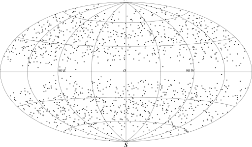
$(b)$

Figure 13: Equal-area plot of the aphelion directions of the $V_{1}$ comets in the Galactic frame. More precisely, we have plotted the antipode of the perihelion direction, since this is what is observable.

The distributions of perihelion and angular orbital elements for the $V_{1}$ comets are shown in Fig. 12, which can be compared to the observed distributions in Fig. 8. The observed perihelion distribution is strongly affected by selection effects, so no comparison is practical there. The angular element distributions are reasonably consistent between the two figures; in particular the $\tilde{\omega}$ distributions both show peaks in the regions where $\sin 2\tilde{\omega}>0$, reflecting the role of the Galactic tide in creating new comets.

The aphelion directions of the $V_{1}$ comets are shown in Fig. 13, which can be compared to the observed distribution in Fig. 9. The most striking feature in Fig. 13 is the concentration towards mid-Galactic latitudes, again pointing to the importance of the Galactic tide as a LP comet injector. The real distribution of aphelion directions is expected to be much clumpier, due to the injection of comets by passing stars; however, the number of new comets in Fig. 9 is too small for any reliable comparisons to be made.

5.1.1 The longest-lived comets

Although most comets reach one of the end-states within a few orbits (see Table I) a small fraction survive for much longer times: 57 of the 20 286 initial comets in our simulation triggered the Exceeded Orbit Limit flag after 5000 orbits. The population of these comets decays only very slowly and their fate cannot be determined without prohibitive expenditures of CPU time. The perihelion distances and semimajor axes of these comets on their 5000^th orbit are indicated in Fig. 14. Also shown is the distance at which they cross the ecliptic. Most have nodes and perihelia outside Saturn’s orbit, where the energy perturbations are relatively small.

Figure 14: For the 57 comets that survived 5000 orbits, ($a$) their perihelion distance $q$ versus semimajor axis $a$, and ($b$) the distances of their nodes. In ($a$), triangles are prograde comets, squares, retrograde.

5.2 Post-visibility evolution: the standard model

We now follow the orbits of the $V_{1}$ comets forward in time until they reach one of the end-states (obviously, the visible end-state is disabled in these simulations). Each time one of these comets makes an apparition its orbital elements are added to the set of $V_{\infty}$ comets. The $V_{\infty}$ comets are to be compared to the observed distribution of LP comets.

The errors in the distribution of elements of the $V_{\infty}$ comets are not Poisson, as a single comet may contribute hundreds or thousands of apparitions. The errors that we quote and show in the figures are determined instead by bootstrap estimation Efron (1982); Press et al. (1992).

The “standard model” simulation of post-visibility evolution has no fading, and no perturbers except the giant planets and the Galactic tide.

The distribution of end-states for the standard model is shown in Table III. The Exceeded orbit limit end-state (§ 4.4) is invoked after 10 000 orbits for these simulations, but no comets reach this end-state. The mean lifetime is 45.3 orbits, compared to 60 predicted by the gambler’s ruin model (Eq. 13). Ejection by the giant planets is by far the most common end-state (89% of $V_{1}$ comets). Most of the remaining comets (about 8% of the total) move back out to large perihelion distances. Their median energy when they reach this end-state is given by $1/a=4\times 10^{-5}$  AU^-1 ($a=25~{}000$  AU); in other words these comets have suffered relatively small energy perturbations and remain in the outer Oort cloud.

The distribution of orbital elements of the $V_{\infty}$ comets may be parametrized by the dimensionless ratios $X_{i}$ defined in Eq. 3: the ratio of theoretical parameters $\Psi_{i}^{t}$ for the standard model to the observed parameters (Eq. 2.8) is

$$X_{1}={\Psi_{1}^{t}\over\Psi_{1}}=0.075\pm 0.011,\qquad X_{2}={\Psi_{2}^{t}\over\Psi_{2}}=4.4\pm 1.2,\qquad X_{3}={\Psi_{3}^{t}\over\Psi_{3}}=0.61\pm 0.13.$$ (51)

The standard model agrees much better with the predictions of the simple gambler’s ruin model ($X_{1}=0.05$, $X_{3}=0.58$, see eqs. 16 and 17) than it does with the observations ($X_{i}=1$).

End-state Ejection Large $q$ Short pd. Total Number 1223 109 36 1368 Fraction 0.894 0.080 0.026 1.000 Minimum $t_{x}$ 0.296 2.61 0.014 0.014 Median $t_{x}$ 1.33 4.62 0.67 1.40 Maximum $t_{x}$ 31.7 71.0 7.94 71.0 Minimum $m_{x}$ 1 1 13 1 Median $m_{x}$ 1 2 330 1 Maximum $m_{x}$ 5832 2158 4277 5832

Table III: The distribution of end-states of the $V_{1}$ comets in the standard model. The minimum, median and maximum lifetimes $t_{x}$ of these comets are measured from their first apparition in Myr. No comets suffer collisions with the planets or Sun, or survive for the age of the Solar System.

The perihelion distribution of the $V_{\infty}$ comets in the standard model is shown in Fig. 15. Although the figure represents 52 303 apparitions, the error bars—as determined by bootstrap—remain large, reflecting strong contributions from a few long-lived comets: over 45% of the apparitions are due to the 12 comets that survive for 1000 or more orbits after their first apparition. This figure can be compared to the observed perihelion distribution (Fig. 2), which however reflects the strong selection effects favouring objects near the Sun or the Earth. We note that not all perihelion passages made by comets after their first apparition are visible: in addition to the 52 303 apparitions made by the $V_{\infty}$ comets, there were 9561 perihelion passages with $q>3{\rm\,AU}$.

Let the total number of comets with perihelia in the range $[q,q+dq]$ be $N(q)dq$. A linear least-squares fit to Fig. 15 yields $N(q)$ roughly proportional to $1+(q/1{\rm\,AU})$, similar to Everhart’s (1967a) earlier estimate of the intrinsic perihelion distribution. The perihelion distribution is not flat, as would be expected if the distribution were uniform on the energy hypersurface (Eq. 4). The simulations are noisy enough to be consistent with any number of slowly varying functions of perihelion over $0<q<3$  AU, possibly including $N(q)\propto q^{1/2}$, as proposed by Kresák and Pittich (1978). The estimates of the intrinsic perihelion distribution of LP comets published by Everhart, by Kresák and Pittich, and by Shoemaker and Wolfe are indicated on Fig. 15.

Figure 15: Distribution of perihelion distances $q$ for the $V_{\infty}$ comets in the standard model. Error bars are determined from bootstrap estimators and represent one standard deviation. The curves are Everhart’s (1967a, dotted line), Kresák and Pittich’s (1982, solid line) and Shoemaker and Wolfe’s (1982, dashed line) estimates of the intrinsic perihelion distribution. The correct normalizations are unclear, and have been made somewhat arbitrarily.

The original energy distribution of the $V_{\infty}$ comets in the standard model is shown in Fig. 16, at two different magnifications, for all 52 303 apparitions. These figures should be compared with the observations shown in Fig. 1. As already indicated by the statistic $X_{1}$ (Eq. 51), the standard model has far too many LP comets relative to the number of comets in the Oort spike: the simulation produces 35 visible LP comets for each comet in the spike, whereas in the observed sample the ratio is 3:1. This disagreement is at the heart of the fading problem: how can the loss of over 90% of the older LP comets be explained?

                                $(a)$ $(b)$

Figure 16: Distribution of original energies for the $V_{\infty}$ comets in the standard model for all 52 303 apparitions ($q<3$  AU).

These simulations allow us to estimate the contamination of the Oort spike by dynamically older comets. There are 1368 $V_{1}$ comets, of which 1340 have $1/a<10^{-4}\hbox{{\rm\,AU}${}^{-1}$}$, but a total of 1475 apparitions are made in this energy range in the standard model. Thus roughly 7% of comets in the Oort spike are not dynamically new. Of course, this estimate neglects fading, which would further decrease the contamination of the Oort spike by older comets.

Figure 17 shows the inclination distribution of the $V_{\infty}$ comets in the standard model. There is a noticeable excess of comets in ecliptic retrograde orbits: the fraction on prograde orbits is $15875/52303\approx 0.3$. This is inconsistent with observations, which show an isotropic distribution (Fig. 3a), but consistent with the predictions of the gambler’s ruin model (Eq. 17).

                                $(a)$ $(b)$

Figure 17: Distribution of the cosine of the inclination for the $V_{\infty}$ comets in the standard model, (a) at perihelion in the ecliptic frame, and (b) at 200  AU on the inbound leg in the Galactic frame. The heavy line indicates a uniform distribution.

Figure 18 shows the distribution of the longitude of the ascending node and the argument of perihelion, in the ecliptic frame. The large error bars suggest that the structure in these figures is probably not statistically significant.

                                $(a)$ $(b)$

Figure 18: Distribution of the longitude of the ascending node and the argument of perihelion for the $V_{\infty}$ comets in the standard model. The elements are measured at perihelion in the ecliptic frame. The heavy line indicates a uniform distribution.

The principal conclusion from this analysis is that the standard model provides a poor fit to the observed distribution of LP comets. The standard model agrees much better with models based on a one-dimensional random walk, suggesting that the basic assumptions of the analytic random-walk models in §3.3 are valid. In §§5.3–5.5 we shall explore whether variants of the standard model can provide a better match to the observations.

5.2.1 Short-period comets from the Oort cloud

During our simulations only 68 Oort cloud comets eventually become short-period comets, 36 of them after having made one or more apparitions as LP comets. The distributions of inverse semimajor axis, perihelion distance and inclination for these comets are shown in Fig. 19. In no case is an Oort cloud comet converted to a short-period comet in a single perihelion passage: the largest orbit at the previous aphelion has a semimajor axis of only 1850  AU. There is a distinct concentration of orbits near zero ecliptic inclination, as expected from studies of captures by Jupiter Everhart (1972), but the concentration is much less than that of short-period comets in our Solar System. The prograde fraction is $44/68\simeq 0.65$.

Figure 19: The distribution of the inverse semimajor axis $1/a$, perihelion distance $q$ and cosine of the ecliptic inclination $i$ for the short-period comets originating in the Oort cloud. The distribution of $1/a$ on the left is measured at the aphelion previous to, and the other distributions measured at, the initial perihelion passage as a short-period comet.

Our simulation corresponds to approximately 450 years of real time (Eq. 49). Thus we deduce that $68/450\simeq 0.15$ short-period comets per year arrive (indirectly) from the Oort cloud (in the absence of fading). For comparison, on average five new short-period comets are discovered each year Festou et al. (1993a); we conclude that the Oort cloud contributes less than 3% of the population of short-period comets, and another source, such as the Kuiper belt, is required. Only about 10% of the known SP comet apparitions are Halley-family, and thus the Oort cloud may contribute a significant fraction of these objects, though the picture is clouded by the multiple apparitions by individual comets in this sample.

5.2.2 Planetary encounter rates

Close encounters of the $V_{\infty}$ comets with the giant planets are described in Table IV. Note the high frequency of multiple encounters between a giant planet and a single comet, though this does not indicate capture by the planet in the traditional sense (i.e. planetocentric eccentricity less than unity).

Planet Sun Jupiter Saturn Uranus Neptune Total Number of comets 7 28 12 2 3 52 Number of encounters 16 43 16 4 3 82 Encounters/comet 2.3 1.5 1.3 2.0 1.0 1.6 Collisions 0 0 0 0 0 0 Captures — 0 0 0 0 0 Min. distance ($R_{\scriptscriptstyle I}$) — 0.018 0.086 0.17 0.16 0.018 Min. distance ($R_{p}$) 1.61 12.5 77.9 335 553 12.5 Outer satellite ($R_{p}$) — 326 216 23 222 —

Table IV: Planetary and solar encounter data for the $V_{\infty}$ comets in the standard model (post-visibility stage). The distance to each planet’s outermost satellite is given in the last row.

Since our simulation corresponds to roughly 450 years of real time (Eq. 49) we can calculate the rate of close encounters between the LP comets and the giant planets. During the combined pre- and post-visibility phases of the comets’ evolution, a total of 253 encounters were recorded for Jupiter, 333 for Saturn, 111 for Uranus and 96 for Neptune. These numbers translate to total currents ${\cal J}_{p}$ of 0.56, 0.74, 0.25 and 0.21 comets per year passing through the spheres of influence (Eq. 24) of Jupiter through Neptune respectively.

If we assume that these currents ${\cal J}_{p}$ reflect a uniform flux of LP comets across the sphere of influence of each planet, then the rate of impacts between LP comets and the giant planets can be deduced to be

$$n_{p}={\cal J}_{p}\left(\frac{M_{p}}{M_{\odot}}\right)^{-4/5}\left(\frac{R_{p}}{a_{p}}\right)^{2}\left(1+{2\over 3}{M_{p}\over M_{\odot}}{a_{p}\over R_{p}}\right),$$ (52)

where $a_{p}$ and $R_{p}$ are the planets’ semimajor axis and radius, $M_{p}$ is the planetary mass, and the second term is a crude correction for gravitational focusing, assuming the comets are on nearly parabolic orbits. The resulting collision rates are $1.0\times 10^{-5}$, $5.0\times 10^{-6}$, $2.4\times 10^{-7}$, $1.3\times 10^{-7}$ per year for Jupiter through Neptune respectively. It should be noted that Comet Shoemaker-Levy 9, which collided with Jupiter in July of 1994, was not a LP comet but rather a Jupiter-family comet Benner and McKinnon (1995).

5.3 Post-visibility evolution: the effect of non-gravitational forces

Asymmetric sublimation of volatiles leads to significant non-gravitational (NG) forces on comets. As described in §4.2, we specify NG forces using two parameters $A_{1}$ and $A_{2}$. The parameter $A_{1}$ is proportional to the strength of the radial NG force, and is always positive, as outgassing accelerates the comet away from the Sun. The parameter $A_{2}$ is proportional to the strength of the tangential force, is generally less than $A_{1}$, and may have either sign depending on the comet’s rotation. Comet nuclei are likely to have randomly oriented axes of rotation, with a corresponding random value of $A_{2}$. Rather than make a complete exploration of the available parameter space for $A_{1}$ and $A_{2}$, we shall investigate a few representative cases.

We assume that $|A_{2}|=0.1A_{1}$, and consider two distributions for the sign of $A_{2}$:

1. Half the comets have positive values of $A_{2}$, half negative, and the sign of $A_{2}$ is constant throughout a comet’s lifetime—as if the axis of rotation of the nucleus remained steady throughout the comet’s dynamical lifetime.

2. The sign of $A_{2}$ is chosen at random after each perihelion passage—as if the axis of rotation changed rapidly and chaotically.

We examined four values of $A_{1}$: $10^{-8},10^{-7},10^{-6},10^{-5}{\rm\,AU}$ day^-2. The first two of these are reasonably consistent with the NG forces observed in LP comets Marsden et al. (1973). The two remaining values for $A_{1}$ are probably unrealistically large.

Figure 20 and Table V illustrate the effects of NG forces on the energy and perihelion distributions, and on the parameters $X_{i}$ defined in Eq. 3, which should be unity if the simulated and observed element distributions agree. The figure shows that NG forces do decrease the number of dynamically older comets relative to the number of new comets and hence improve agreement with the observations (i.e. increasing $X_{1}$, decreasing $X_{2}$); however, the same forces erode the population of comets at small perihelion distances, thereby worsening the agreement with the observed perihelion distribution. Even unrealistically large NG forces cannot bring the distribution of inverse semimajor axes into line with observations, and these produce an extremely unrealistic depletion of comets at small perihelia.

The effects of NG forces can be summarized as follows:

• The semimajor axis perturbation due to radial NG forces averages to zero over a full orbit (assuming that the radial force is symmetric about perihelion, as in the model discussed in §4.2). Thus radial forces have little or no long-term effect on the orbital distribution.

• Positive values of the tangential acceleration $A_{2}$ reduce the tail of the population, resulting in an increase in $X_{1}$ towards unity and improving the match with observations, but erode the population at small perihelia, a depletion which is not seen in the observed sample.

• Negative values of $A_{2}$ preserve a reasonable perihelion distribution, but increase the number of comets in the tail of the energy distribution, thus reducing $X_{1}$ so that the disagreement between the observed and simulated energy distribution becomes even worse.

We have also conducted simulations with a more realistic model for observational selection effects (Eq. 1) but this does not alter our conclusions.

Although we have not exhaustively explored the effects of NG forces on the LP comet distribution, we are confident that conventional models of NG forces cannot by themselves resolve the discrepancy between the observed and predicted LP comet distribution.

 

Figure 20: Distribution of the inverse semimajor axis $1/a$ and perihelion distance $q$ for $V_{\infty}$ comets subjected to non-gravitational forces. Left panels: constant values for $A_{2}$, half positive, half negative. Right panels: the sign of $A_{2}$ is randomised for each perihelion passage. From the top down, $A_{1}=10^{-8}$, $10^{-7}$, $10^{-6}$ and $10^{-5}$  AU day^-2, with $|A_{2}|=0.1A_{1}$. The bottom line of panels is for comparison, and includes the standard model (left side) and the observations (right side). The observed perihelion distribution includes curves indicating the estimated intrinsic distribution (see Fig. 15 for details).

$A_{1}$ $A_{2}$ Total Spike Tail Prograde $X_{1}$ $X_{2}$ $X_{3}$ $\langle m\rangle$ 0.0 0.0 52303 1473 15004 15875 0.07 4.37 0.61 45.4 1.0 0.1 35370 1457 7368 12381 0.11 3.17 0.70 36.1 1.0 $-0.1$ 57819 1462 19364 21110 0.07 5.10 0.73 51.0 1.0 $\pm 0.1^{a}$ 44383 1461 13705 19021 0.09 4.70 0.86 38.4 10 $\pm 1^{a}$ 45899 1425 16628 18504 0.08 4.42 0.80 42.5 100 $\pm 10^{a}$ 30660 1341 11296 11012 0.12 5.61 0.72 33.1 1000 $\pm 100^{a}$ 13248 995 5432 5872 0.20 6.24 0.88 14.4 1.0 $\pm 0.1^{b}$ 49642 1450 13203 16387 0.08 4.05 0.66 46.7 10 $\pm 1^{b}$ 45202 1448 13631 17311 0.08 4.59 0.76 41.4 100 $\pm 10^{b}$ 25774 1364 4969 11452 0.14 2.93 0.88 27.7 1000 $\pm 100^{b}$ 9878 1035 1536 5042 0.28 2.37 1.02 13.2

Table V: Parameters of the distribution of $V_{\infty}$ comets subjected to non-gravitational forces. The superscript ^a indicates that half the sample have positive $A_{2}$, half negative; ^b indicates that $A_{2}$ has a randomly chosen sign for each perihelion passage. “Total” is the total number of apparitions (i.e. perihelion passages with $q<3$  AU), “Spike” is the number of these with original inverse semimajor axes $1/a<10^{-4}\hbox{{\rm\,AU}${}^{-1}$}$, “Tail” is the number with $0.0145\hbox{{\rm\,AU}${}^{-1}$}<1/a<0.029\hbox{{\rm\,AU}${}^{-1}$}$, and “Prograde” the number with ecliptic inclination less than $90^{\circ}$. The parameters $X_{i}$ are defined in Eq. 3. The mean lifetime in orbits $\langle m\rangle$ includes all perihelion passages, whether visible or not, after the initial apparition. The units of $A_{1}$ and $A_{2}$ are AU day^-2.

5.4 Post-visibility evolution: the effect of a solar companion or disk

In this section we investigate the influence of two hypothetical components of the Solar System on the evolution of LP comets:

1. A massive circumsolar disk extending to hundreds of ${\rm\,AU}$ or even further. Such a disk might be an extension of the Kuiper belt Jewitt et al. (1996) or related to the gas and dust disks that have been detected around stars (especially $\beta$ Pictoris) and young stellar objects (Ferlet and Vidal-Madjar 1994). Residuals in fits to the orbit of Halley’s comet imply that the maximum allowed mass for a disk of radius $r$ is roughly Hogg et al. (1991)

   $$M_{\rm max}\simeq 10M_{\oplus}\left(r\over 100{\rm\,AU}\right)^{3}.$$ (53)

   Current estimates of the mass in the Kuiper belt are much smaller, typically $\sim 0.1M_{\oplus}$ from direct detection of 100 km objects Jewitt et al. (1996) or from models of diffuse infrared emission Backman et al. (1995), but these are based on the uncertain assumption that most of the belt mass is in the range 30–50${\rm\,AU}$. The disk around $\beta$ Pic is detected in the infrared to radii exceeding 1000  AU Smith and Terrile (1987); the dust mass is probably less than $1M_{\oplus}$ Artymowicz (1994), but there may be more mass in condensed objects.

2. A solar companion, perhaps a massive planet or brown dwarf, orbiting at hundreds of ${\rm\,AU}$. Residuals in fits to the orbits of the outer planets imply that the maximum allowed mass for a companion at radius $r$ is roughly Tremaine (1990); Hogg et al. (1991)

   $$M_{\rm max}\simeq 100M_{\oplus}\left(r\over 100{\rm\,AU}\right)^{3}.$$ (54)

   There are also significant but model-dependent constraints on the characteristics of a solar companion from the IRAS infrared all-sky survey Hogg et al. (1991).

To reduce computational costs, we used the $V_{1}$ comets as a starting point for these investigations; that is, the effect of the disk or companion is ignored before the comet’s first apparition (more precisely, we started the integration at the aphelion preceding the comet’s initial apparition, in order to correctly calculate any perturbations occurring on the inbound leg). Starting at this point is an undesirable oversimplification, but one that should not compromise our conclusions.

5.4.1 Circumsolar disk

The circumsolar disk is represented by a Miyamoto-Nagai potential (Binney and Tremaine, 1987, e.g. ),

$$V_{\rm disk}(x,y,z)=\frac{-GM_{d}}{\Big{[}x^{2}+y^{2}+\left(a_{d}+\sqrt{z^{2}+b_{d}^{2}}\,\right)^{2}\Big{]}^{1/2}}.$$ (55)

Here $M_{d}$ is the disk mass, and $a_{d}$ and $b_{d}$ are parameters describing the disk’s characteristic radius and thickness. We assume that the disk is centered on the Solar System barycenter and coplanar with the ecliptic. We considered disk masses $M_{d}$ of 0.1, 1, and 10 Jupiter masses, disk radii $a_{d}$ of $100$ and $1000{\rm\,AU}$, and a fixed axis ratio $b_{d}/a_{d}=0.1$. The two more massive disks with $a_{d}=100{\rm\,AU}$ are unrealistic because they strongly violate the constraint (53), but we examine their effects in order to explore as wide a range of parameters as possible.

Comets arriving from the Oort cloud have fallen through the disk potential and hence are subjected to a shift in their original inverse semimajor axis. This offset can be as large as $2\times 10^{-4}$  AU^-1 for a 10 Jupiter-mass disk with radius 100  AU, but is much smaller for disks that do not already violate the observational constraint (53). This shift is not shown in the Figures below, for which the semimajor axis is measured at aphelion.

As usual, the Perihelion Too Large end-state (§ 4.4) was entered if $q>40{\rm\,AU}$ and $\sin 2\tilde{\omega}>0$. The assumption that such comets are unlikely to become visible in the future is only correct if the torque is dominated by the Galactic tide, and this may not be the case when a disk is present. However, there is no significant difference in the numbers or semimajor axes of the comets reaching this end-state in simulations with and without a circumsolar disk, suggesting that evolution to this end-state is indeed dominated by the Galaxy.

The results from simulations including a circumsolar disk are displayed in Fig. 21 and Table VI. One plot of the energy distribution in Fig. 21 shows a strong peak near $1/a=0.02\hbox{{\rm\,AU}${}^{-1}$}$; as the large error bars suggest, this peak is caused by a single comet and has little statistical significance.

The principal effect of the disk is to exert an additional torque on the comets, resulting in oscillations of the comet’s perihelion distance. This effect normally increased the comet’s lifetime, as the risk of ejection is greatly reduced when the comet is outside Saturn’s orbit. The perihelion oscillations also enhance the probability of collision with the Sun (Table VI).

The perihelion distribution of visible comets is not strongly affected by the disk. The presence of a massive disk reduces the number of dynamically old comets (because their perihelia are no longer nearly constant, only a fraction of them are visible at any given time), but not enough so that the energy distribution is consistent with the observations. This conclusion is confirmed by examining the $X$ parameters in Table VI, which should be unity if the simulated element distribution agrees with the observations (cf. Eq. 3). The values of $X_{1}$, which measures the ratio of number of comets in the spike to the total number, are far smaller than unity even for the most massive disks. Increasing the disk mass tends to improve $X_{2}$ and $X_{3}$ for the 1000  AU disk, but degrades the fit for the $100{\rm\,AU}$ disk. There is no set of disk parameters than comes close to producing a match with observations. Using a more elaborate model for selection effects (Eq. 1) does not alter this conclusion (see bottom half of Table  VI).

We conclude that a circumsolar disk cannot by itself resolve the discrepancy between the observed and predicted LP comet distribution.

 

Figure 21: Distribution of the inverse semimajor axis $1/a$ and perihelion distance $q$ for the $V_{\infty}$ comets, when the Solar System contains a massive circumsolar disk. Left panels: characteristic disk radius $a_{d}=100$  AU. Right panels: disk radius $a_{d}=1000$  AU. From the top down, the disk masses are 0.1, 1 and 10 Jupiter masses. The bottom line of panels is for comparison, and includes the standard model (left side) and the observations (right side). The observed perihelion distribution includes curves indicating the estimated intrinsic distribution (see Fig. 15 for details).

$M_{d}$ $a_{d}$ Total Spike Tail Prograde $X_{1}$ $X_{2}$ $X_{3}$ $\langle m\rangle$ $R_{\odot}$ 0 — 52303 1473 15004 15875 0.07 4.37 0.61 45.4 0 0.1 100 38947 1486 8382 15178 0.10 3.28 0.78 60.4 0 0.1 1000 42106 1496 9122 16957 0.09 3.30 0.80 33.7 1 1 100 37676 1459 12027 11888 0.10 4.86 0.63 60.8 2 1 1000 39138 1458 9944 16141 0.10 3.87 0.82 44.7 1 10 100 26445 1416 8881 6813 0.14 5.11 0.51 62.6 5 10 1000 16636 1324 3020 7555 0.21 2.76 0.91 66.9 3 $0^{d}$ — 33449 957 10190 14308 0.09 4.17 0.83 45.5 0 $0.1^{d}$ 100 24535 968 6086 8589 0.10 3.76 0.70 60.4 0 $0.1^{d}$ 1000 26335 969 5261 11950 0.10 3.04 0.91 33.7 1 $1^{d}$ 100 27655 947 9514 8712 0.09 5.24 0.63 60.8 2 $1^{d}$ 1000 25200 947 7070 9881 0.10 4.27 0.78 44.7 1 $10^{d}$ 100 18769 939 7104 4103 0.13 5.76 0.44 62.6 5 $10^{d}$ 1000 10600 910 1541 4650 0.23 2.21 0.86 66.9 3

Table VI: Parameters of the distribution of $V_{\infty}$ comets, when the Solar System contains a circumsolar disk. The disk mass $M_{d}$ is measured in Jupiter masses and the disk radius $a_{d}$ is measured in ${\rm\,AU}$. The rightmost column indicates the number of comets that collided with the Sun. The superscript ^d indicates that the discovery probability from Eq. 1 has been applied. The definitions of the other columns are the same as in Table V.

5.4.2 Solar companion

For simplicity, we shall assume that the solar companion has a circular orbit in the ecliptic (the orientation and eccentricity of the companion orbit should not strongly affect its influence on the LP comets since the comets are on isotropic, highly eccentric robits).

We examined companion masses $M_{X}$ of 0.1, 1 and 10 Jupiter masses and orbital radii of 100 and 1000  AU. The most massive companion at $100{\rm\,AU}$ is unrealistic because it strongly violates the constraint (54). As in the previous subsection, the original semimajor axes of the comets are measured at aphelion, and thus do not include the energy offset caused by their fall through the companion’s gravitational potential.

The results are presented in Fig. 22 and Table VII. The $X$ parameters are listed in Table VII. As the companion mass is increased, the fraction of prograde to total comets ($X_{3}$) improves. However, $X_{1}$ and $X_{2}$ remain far from unity. There is no evidence that a solar companion can significantly improve the agreement between the observed and predicted LP comet distribution.

 

Figure 22: Distribution of the inverse semimajor axis $1/a$ and perihelion distance $q$ for the $V_{\infty}$ comets, when the Solar System contains a massive solar companion. Left panels: companion orbital radius of $100$  AU. Right panel: orbital radius $1000{\rm\,AU}$. From the top down, the companion masses are 0.1, 1 and 10 Jupiter masses. The bottom line of panels is for comparison, and includes the standard model (left side) and the observations (right side). The observed perihelion distribution includes curves indicating the estimated intrinsic distribution (see Fig. 15 for details).

$M_{X}$ $a_{X}$ Total Spike Tail Prograde $X_{1}$ $X_{2}$ $X_{3}$ $\langle m\rangle$ $R_{\odot}$ 0.1 100 40662 1451 9111 14074 0.11 3.07 0.67 43.1 1 0.1 1000 49420 1490 10057 13550 0.09 2.79 0.53 44.4 1 1 100 38397 1473 7465 9379 0.12 2.66 0.47 85.4 4 1 1000 35940 1438 9338 13544 0.12 3.56 0.73 68.1 1 10 100 14877 1379 3365 5846 0.28 3.10 0.76 66.0 4 10 1000 28600 1400 8183 15489 0.15 3.92 1.05 146.3 2 0.1^d 100 25300 944 6762 8893 0.11 3.66 0.68 43.1 1 0.1^d 1000 31376 975 6206 8623 0.09 2.71 0.53 44.4 1 1^d 100 27918 963 4764 6047 0.10 2.34 0.42 85.4 4 1^d 1000 24740 943 6713 8281 0.12 3.72 0.65 68.1 1 10^d 100 9749 928 2197 4059 0.29 3.09 0.81 66.0 4 10^d 1000 22177 1030 6052 12649 0.14 3.74 1.11 146.3 2

Table VII: Parameters of the distribution of $V_{\infty}$ comets, when the Solar System contains a massive solar companion. The companion mass $M_{X}$ is in Jupiter masses, and its orbital radius $a_{X}$ is measured in ${\rm\,AU}$. The rightmost column indicates the number of comets that collided with the Sun. The superscript ^d indicates that the discovery probability from Eq. 1 has been applied. The definitions of the other columns are the same as in Table V.

5.5 Post-visibility evolution: fading

The concept of fading was introduced in §§3.3 and 3.4. We use the term “fading” to denote any change in the intrinsic properties of the comet that would cause it to disappear from the observed sample. Our focus is on modeling the fading process empirically, rather than attempting to elucidate the physical processes involved. The distributions of inverse semimajor axis and ecliptic inclination will serve as our primary fading benchmarks, through the values of the parameters $X_{1}$, $X_{2}$ and $X_{3}$ (Eq. 3).

We shall generally assume that fading depends only on the number of apparitions (perihelion passages with $q<3{\rm\,AU}$). We parametrize the fading process by a function $\Phi_{m}$ (cf. Eq. 9), the probability that a visible new comet survives fading for at least $m$ apparitions (thus $\Phi_{1}=1$).

We shall conduct simulations with and without plausible non-gravitational (NG) forces (§§4.2, 5.3). When NG forces are included, we shall use the parameters $A_{1}=10^{-7}$  AU day^-2, $A_{2}=\pm 10^{-8}$  AU day^-2, $A_{3}=0$, with a random sign for $A_{2}$ at each perihelion passage (henceforth the “standard NG model”).

The most direct way to determine the fading function $\Phi_{m}$ would be to break down the simulated data set into individual distributions, one for each perihelion passage i.e. $\{V_{1},V_{2},V_{3},\ldots\}$, and then fit the observed distribution of orbital elements to the parameters $\Phi_{1},\Phi_{2},\ldots$ where $\Phi_{m+1}\leq\Phi_{m}$. Unfortunately, this problem is poorly conditioned. Instead, we shall experiment with a few simple parametrized fading functions.

5.5.1 One-parameter fading functions

The fading functions we shall examine include:

a) Constant lifetime

Each comet is assigned a fixed lifetime, measured in apparitions. Thus

$$\Phi_{m}=1,\quad m\leq m_{v},\qquad\qquad\Phi_{m}=0,\quad m>m_{v}.$$ (56)

b) Constant fading probability

Comets are assigned a fixed probability $\lambda$ of fading, per apparition. Thus

$$\Phi_{m}=(1-\lambda)^{m-1}.$$ (57)

c) Power-law

The fraction of comets remaining is

$$\Phi_{m}=m^{-\kappa},$$ (58)

where $\kappa$ is a positive constant.

We have also investigated fading functions in which $\Phi$ depends on the elapsed time $t$ since the first apparition. Such laws are less physically plausible than fading functions based on the number of apparitions, since by far the harshest environment for comets occurs as they pass perihelion; and in fact the functions $\Phi(t)$ that we investigated all produced relatively poor matches to the observations. Also, fading functions in which $\Phi$ depends on the number of perihelion passages produce results very similar to laws based on the number of apparitions.

The results from the fading laws (56)–(58) are shown in Figs. 23 to 25. The first of these figures displays the $X$ parameters assuming LP comets have a constant lifetime in apparitions (model [a]). The presence or absence of NG forces (bottom vs. top panels), or the use of two different visibility criteria (left vs. right panels) has very little effect on the results. The spike/total ratio matches observations (i.e. $X_{1}=1$) at $m_{v}\simeq 10$, but the tail/total ratio is far too low at that point ($X_{2}\ll 1$). The tail/total ratio is right at $m_{v}\simeq 100$, but $X_{1}$ is now too low. The ratio $X_{3}$ is typically close to but below unity. The model does not match the observations for any value of the parameter $m_{v}$.

Figure 23: The values of the parameters $X_{i}$ for a fading function with a fixed lifetime of $m_{v}$ apparitions (model [a], Eq. 56). If the simulation agrees with the observations then $X_{i}=1$, $i=1,2,3$. The parameter $X_{1}$ is based on the fraction of LP comets in the Oort spike (solid curve); $X_{2}$ is based on the fraction of comets in the energy tail, $x>0.0145\hbox{{\rm\,AU}${}^{-1}$}$ (dotted curve); $X_{3}$ is based on the fraction of prograde comets (dashed curve) (cf. §2.8). The panels on the left are based on the visibility criterion $q<3{\rm\,AU}$, and those on the right are based on the visibility probability (Eq. 1). The upper panels are based on the standard model with no NG forces, and the lower panels are based on the standard NG model.

Figure 24: The values of $X_{i}$ given a fixed fading probability $\lambda$ per apparition (model [b], Eq. 57). For further details see the caption to Fig. 23.

Figure 25: The values of $X_{i}$ given a power-law fading function with exponent $-\kappa$ (model [c], Eq. 58). For further details see the caption to Fig. 23.

Figure 24 displays the behaviour of the parameters $X_{i}$ given a fixed fading probability $\lambda$ per apparition (model [b]). Once again, the results are almost independent of NG forces and the visibility criterion, and there is no value for the parameter $\lambda$ that matches the observations ($X_{i}=1$).

Figure 25 shows the parameters $X_{i}$ for a power-law fading function (model [c]). Although the match is not perfect, an exponent $\kappa=0.6\pm 0.1$ provides a much better match than the previous two models: $X_{1}=0.73\pm 0.09$, $X_{2}=0.96\pm 0.26$, and $X_{3}=0.95\pm 0.12$ when the standard NG model and discovery probability (Eq. 1) are used. The distributions of orbital elements are shown in Fig. 26, to be compared with the observed distributions in § 2. For $m\gg 1$ this fading law is the same as an empirical law suggested by Whipple (1962), $\phi_{m}\equiv\Phi_{m}-\Phi_{m+1}\propto m^{-\kappa-1}$; Whipple estimated $\kappa=0.7$.

Figure 26: The distribution of the inverse semimajor axis $1/a$, perihelion distance $q$ and cosine of the ecliptic inclination $i$ for a power-law fading function with exponent $\kappa=-0.6$ (Eq. 58). These simulations are based on the standard NG model and the visibility probability in Eq. 1.

5.5.2 Other fading functions

We have also examined several two-parameter fading functions:

d) Two populations

Suppose that the Oort cloud contains two populations of comets, distinguished by their internal strength. The first and more fragile set is disrupted after $m_{v}$ apparitions, while the more robust comets, comprising a fraction $f$ of the total, do not fade at all. Thus

$$\Phi_{m}=1,\quad m\leq m_{v},\qquad\qquad\Phi_{m}=f,\quad m>m_{v}.$$ (59)

e) Constant fading probability plus survivors

One population has a fixed fading probability $\lambda$ per apparition, while the more robust comets, comprising a fraction $f$ of the total, do not fade at all. Thus

$$\Phi_{m}=(1-f)(1-\lambda)^{m-1}+f.$$ (60)

f) Offset power law

The fading function is chosen to be

$$\Phi_{m}=[(m+\beta)/(1+\beta)]^{-\kappa},$$ (61)

Figure 27: The values of $X_{i}$ given a two-parameter fading function in which a fraction $1-f$ survives for $m_{v}$ apparitions, while a fraction $f$ survives forever (model [d], Eq. 59). The fractions $f$ for the different curves are 0, 0.01, 0.04, 0.07, 0.1, 0.2, 0.4, 0.6, 0.8 and 1, beginning with the heavy lines. For further details see the caption to Fig. 23.

The results of model (d) are shown in Fig. 27. In most cases the fit is worse than in the one-parameter model (a), shown by the heavy lines, because the prograde fraction described by $X_{3}$ is lower when some of the comets do not fade. The best match is for the standard NG model with visibility probability (1) (lower right panel). Here the parameters $m_{v}=6$, $f=0.04$ yield $X_{1}=0.83\pm 0.10$, $X_{2}=0.91\pm 0.26$, $X_{3}=0.96\pm 0.11$, slightly better than the match for model (a). This model is reminiscent of Weissman’s (1978) favoured model, in which 85% of LP comets had significant fading probabilities while the reminder survived indefinitely.

Model (e) is a generalization of the one-parameter model (b) but ordinarily does no better: the match to observations is usually best when the survivor fraction $f$ is set to zero, and gets worse as $f$ increases. Model (f) also does no better than its one-parameter counterpart, model (c).

Finally, we examine

g) Other published fading functions:

In § 3.3, we described a number of fading functions deduced in previous studies. Oort (1950) took $\psi_{1}=0.8$, $\psi_{m}=0.014$ for $m>1$; Kendall (1961) took $\psi_{1}=0.8$, $\psi_{m}=0.04$ for $m>1$; Whipple (1962) took $\phi_{m}\propto m^{-1.7}$; Weissman (1978) took $f=0.15$, $\lambda=0.1$ (cf. Eq. 60); Everhart (1979) took $\Phi_{1}=1$, $\Phi_{m}=0.2$ for $m>1$; Bailey’s (1984) fading law is described by Eq. (20); and Emel’yanenko and Bailey (1996) assume $\Phi_{m}=0.3$ but add a probability $k^{\ast}=0.0005$ that the comet is “rejuvenated”. In Table VIII, we have listed the values of $X_{i}$ obtained for all these fading models (the results in the Table are based on the model that includes the discovery probability (1) and standard NG forces; other models give very similar results). Many provide reasonable matches to the data but none do as well as our best fits.

Name $X_{1}$ $X_{2}$ $X_{3}$ Oort $0.66\pm 0.09$ $1.21\pm 0.44$ $0.92\pm 0.13$ Kendall $0.99\pm 0.12$ $0.59\pm 0.23$ $0.92\pm 0.11$ Whipple $0.97\pm 0.11$ $0.58\pm 0.16$ $0.95\pm 0.11$ Weissman $0.50\pm 0.07$ $2.07\pm 0.58$ $0.97\pm 0.14$ Everhart $0.47\pm 0.07$ $2.60\pm 0.72$ $0.97\pm 0.15$ Bailey $0.82\pm 0.11$ $1.68\pm 0.63$ $1.07\pm 0.13$ Emel’yanenko $0.69\pm 0.08$ $0.16\pm 0.05$ $0.94\pm 0.10$

Table VIII: The values of $X_{i}$ for the preferred fading models of Oort (1950), Kendall (1961), Whipple (1962), Weissman (1978), Everhart (1979), Bailey (1984), and Emel’yanenko and Bailey (1996). The results are based on the model which includes the discovery probability (1) and the standard NG forces.

6 Summary

The LP comets provide our only probe of the properties of the Oort comet cloud. The expected distribution of their orbital elements is only weakly dependent on the properties of the Oort cloud and is straightforward—though not easy—to predict if the distribution is in a steady state. Thus a central problem in the study of comets is to compare the predicted and observed distributions of the orbital elements of the LP comets.

We have simulated the dynamical evolution of LP comets from their origin in the Oort cloud until the comets are lost or destroyed. We have integrated the comet trajectories under the influence of the Sun, the giant planets, and the Galactic tide. In some cases we have included the effects of non-gravitational forces, a hypothetical circumsolar disk or solar companion, and the disruption or fading of the comet nucleus. We have not included the effects of passing stars on the Oort cloud; these add a random component to the expected distribution of LP comets which is more difficult to model but is not expected to strongly affect the distribution except during rare comet showers (cf. §4.1.3). Our conclusions from these simulations include the following:

The Oort cloud presently contains roughly $5\times 10^{11}(\Phi_{\rm new}/3\hbox{ yr}^{-1})$ objects orbiting between 10 000 and 50 000  AU from the Sun (Eq. 49), assuming that the cloud is in a steady state and that the number density in the cloud is proportional to $r^{-3.5}$ Duncan et al. (1987); here $\Phi_{\rm new}$ is the observed current of new comets with perihelion $<3{\rm\,AU}$. This estimate depends strongly on uncertain assumptions about the density and extent of the inner Oort cloud; a more reliable parameter is that the number of comets in the outer Oort cloud ($a>20~{}000{\rm\,AU}$) is $4\times 10^{11}(\Phi_{\rm new}/3\hbox{ yr}^{-1})$.

Over 90% of the comets in the Oort spike ($1/a<10^{-4}\hbox{{\rm\,AU}${}^{-1}$}$) are making their first apparition (§5.2), and only 2% of new comets have energies outside the spike (§5.1). The Oort cloud provides only a few percent of the observed short-period comets, and even fewer if LP comets fade. Thus another source, such as the Kuiper belt, must provide the bulk of the short-period comets. On the other hand, a significant fraction of the Halley-family comets may arise in the Oort cloud; however, biases in and the small size of our both the observed and simulated Halley-family comets render this estimate very approximate.

LP comets collide with Jupiter and Saturn roughly once per $10^{5}{\rm\,yr}$ if $\Phi_{\rm new}=3\hbox{ yr}^{-1}$ (§ 5.2.2).

This research does not explain the existence of comets on hyperbolic original orbits (see Fig. 1). The excess velocities are small, corresponding to roughly $-10^{-4}$  AU^-1 in inverse semimajor axis, but are larger than those produced by the Galactic tide ($\sim-10^{-6}$  AU^-1), by plausible non-gravitational forces ($\sim-10^{-5}$  AU^-1) or by a circumsolar disk or solar companion small enough to be compartible with the distribution of bound orbits.

Using simple models based on a one-dimensional random walk (§3.3), many investigators, starting with Oort (1950), have concluded that the observed energy distribution of LP comets is incompatible with the expected steady-state distribution, unless most new comets are destroyed before their second or subsequent perihelion passage. We have shown that this “fading” problem persists in a simulation that follows the comet orbits in detail.

Non-gravitational forces play a significant role in shaping the distributions of the orbital elements of the LP comets, but are too small by at least two orders of magnitude to resolve the fading problem (§4.2). Hypothetical additional components of the Solar System such as a massive circumsolar disk or solar companion also do not resolve the fading problem (§5.4).

We can match the observed distribution of orbital elements to the expected steady-state distribution with at least two fading functions: (a) a one-parameter power-law (Eq. 58) with exponent $\kappa\simeq 0.6$ Whipple (1962); (b) a two-population model (Eq. 59) in which approximately 95% of comets survive for roughly six orbits and the remainder do not fade (the latter model is also roughly consistent with the observed splitting probabilities of dynamically new LP comets, approximately 0.1 per orbit; see Weissman 1980). The observation that the cratering rate is roughly compatible with the rate expected from the current known populations of comets and asteroids (§ 3.4) suggests—within the large uncertainties—that fading occurs through the fragmentation or disruption of the comet nucleus rather than through the production of a single “dead” body. We also note the lack of strong fading in new comets during single perihelion passage, which might be expected if fading were due to loss of volatiles from an intact nucleus. One possible model compatible with these observations is that the nucleus of a new comet fragments during its first apparition, but that the separation velocity of the fragments is small enough that they remain within the coma until well past observability.

Although physically plausible, fading remains an ad hoc explanation for the distribution of LP comet orbits which has not been independently confirmed, and we should remain alert for other possible explanations.

We thank Tom Bolton, Ray Carlberg, Martin Duncan, Bob Garrison and Kim Innanen for helpful discussions and advice. This research was performed at the University of Toronto and the Canadian Institute for Theoretical Astrophysics, and has been supported in part by the Natural Sciences and Engineering Research Council of Canada.

References

- Artymowicz (1994) Artymowicz, P. 1994. Modeling and understanding the dust around Pictoris. In Circumstellar Dust Disks and Planet Formation, R. Ferlet and A. Vidal-Madjar (eds.), pages 47–65. Gif sur Yvette: Editions Frontières.
- Backman et al. (1995) Backman, D. E., Dasgupta, A., and Stencel, R. E. 1995. Model of a Kuiper belt small grain population and resulting far infrared emission. Astrophys. J. Lett. 450:35–38.
- Bahcall et al. (1992) Bahcall, J. N., Flynn, C., and Gould, A. 1992. Local dark matter density from a carefully selected sample. Astrophys. J. 389:234–250.
- Bahcall (1984) Bahcall, J. N. 1984. Self-consistent determinations of the total amount of matter near the Sun. Astrophys. J. 276:169–181.
- Bailey et al. (1992) Bailey, M. E., Chambers, J. E., and Hahn, G. 1992. Origin of sungrazers – a frequent cometary end-state. Astron. Astrophys. 257:315–322.
- Bailey (1983) Bailey, M. E. 1983. The structure and evolution of the Solar System comet cloud. Mon. Not. Roy. Astron. Soc. 204:603–633.
- Bailey (1984) Bailey, M. E. 1984. The steady-state distribution and the problem of cometary fading. Mon. Not. Roy. Astron. Soc. 211:347–368.
- Benner and McKinnon (1995) Benner, L. A. M. and McKinnon, W. B. 1995. On the orbital evolution and origin of Comet Shoemaker-Levy 9. Icarus 118:155–168.
- Binney and Tremaine (1987) Binney, J. and Tremaine, S. 1987. Galactic Dynamics. Princeton: Princeton University Press.
- Carusi and Valsecchi (1992) Carusi, A. and Valsecchi, G. B. 1992. Dynamics of comets. In Chaos, Resonance and Collective Dynamical Phenomena in the Solar System, S. Ferraz-Mello (ed.), pages 255–268.
- Chirikov and Vecheslavov (1989) Chirikov, B. V. and Vecheslavov, V. V. 1989. Chaotic dynamics of comet Halley. Astron. Astrophys. 221:146–154.
- Delsemme and Miller (1971) Delsemme, A. H. and Miller, D. C. 1971. Physico-chemical phenomena in comets. III. The continuum of comet Burnham (1960 II). Plan. Space Sci. 19:1229–1257.
- Drapatz and Zinnecker (1984) Drapatz, S. and Zinnecker, H. 1984. The size and mass distribution of galactic molecular clouds. Mon. Not. Roy. Astron. Soc. 210:11–14.
- Duncan et al. (1987) Duncan, M., Quinn, T., and Tremaine, S. 1987. The formation and extent of the Solar System comet cloud. Astron. J. 94:1330–1338.
- Efron (1982) Efron, B. 1982. The Jackknife, the Bootstrap and Other Resampling Plans. Philadelphia: Society for Industrial and Applied Mathematics.