A PHASE-SPACE APPROACH TO COLLISIONLESS
STELLAR SYSTEMS USING A PARTICLE METHOD

Abstract

A particle method for reproducing the phase space of collisionless stellar systems is described. The key idea originates in Liouville’s theorem which states that the distribution function (DF) at time $t$ can be derived from tracing necessary orbits back to $t=0$. To make this procedure feasible, a self-consistent field (SCF) method for solving Poisson’s equation is adopted to compute the orbits of arbitrary stars. As an example, for the violent relaxation of a uniform-density sphere, the phase-space evolution which the current method generates is compared to that obtained with a phase-space method for integrating the collisionless Boltzmann equation, on the assumption of spherical symmetry. Then, excellent agreement is found between the two methods if an optimal basis set for the SCF technique is chosen. Since this reproduction method requires only the functional form of initial DFs but needs no assumptions about symmetry of the system, the success in reproducing the phase-space evolution implies that there would be no need of directly solving the collisionless Boltzmann equation in order to access phase space even for systems without any special symmetries. The effects of basis sets used in SCF simulations on the reproduced phase space are also discussed.

1 INTRODUCTION

N-body simulations have become a powerful tool for numerical studies of self-gravitating systems. In fact, they have provided us with such significant results as the bar instability in disk galaxies (e.g., Hohl 1971; Ostriker & Peebles 1973) and the radial orbit instability in spherical stellar systems (e.g., Barnes, Goodman, & Hut 1986). Much of knowledge obtained with N-body methods is essentially based on the change in, and the evolution of, the shape of the system. However, as far as collisionless stellar systems like galaxies are concerned, phase-space arguments, which take into consideration velocity space as well as configuration space, help us understand the physics of them. As argued by Fujiwara (1983a) in his appendix, the core size of collapsed objects can be estimated from the conservation of phase-space density. In addition, such a phase-space constraint was also applied to the explanation of why the tangential velocity dispersion, in general, grows faster than the radial one at the early stages of gravitational collapse for spherical systems; consequently, the initial anisotropy in velocity dispersion was shown to be a poor indicator of the radial orbit instability (Hozumi, Fujiwara, & Kan-ya 1996).

Although the phase-space approach is useful for collisionless stellar dynamics, it is difficult to access phase space numerically: such systems are governed by the collisionless Boltzmann equation,

$$\frac{\partial f}{\partial t}+\mbox{\boldmath$v\cdot$}\frac{\partial f}{\partial\mbox{\boldmath$r$}}-\nabla\Phi\mbox{\boldmath$\cdot$}\frac{\partial f}{\partial\mbox{\boldmath$v$}}=0,$$ ()

and Poisson’s equation,

$$\nabla^{2}\Phi(\mbox{\boldmath$r$})=4\pi G\rho(\mbox{\boldmath$r$}),$$ ()

where $f=f(\mbox{\boldmath$r$}(t),\mbox{\boldmath$v$}(t),t)$ is the distribution function (DF), $\Phi$ the potential, $\rho$ the density, $r$ the position vector, $v$ the velocity vector, $t$ the time, and $G$ the gravitational constant. Thus, collisionless systems in general configurations must be described in six-dimensional phase space. It is, therefore, practically impossible to solve equations (1) and (2) numerically due to memory limitations of currently available computers. One then has to approximate the system in a simpler form. In fact, the collisionless Boltzmann equation has been solved numerically only for one-dimensional systems (Fujiwara 1981; Mineau, Feix, & Rouet 1990; White 1986), two-dimensional disk systems (Watanabe et al. 1981; Nishida et al. 1981, 1984; Nishida 1986), and spherically symmetric systems (Hoffman, Shlosman, & Shaviv 1979; Shlosman, Hoffman, & Shaviv 1979; Fujiwara 1983a, 1983b; Rasio, Shapiro, & Teukolsky 1989). In spite of such simplification, the phase-space approach is indeed superior to conventional N-body methods: phase-space holes became indiscernible as time proceeded with an N-body code but were kept long-lived with a phase-space code (Mineau et al. 1990). Above all, Fujiwara (1983a) has demonstrated clearly how violent relaxation, together with the subsequent phase mixing, proceeds in phase space, and that the resulting DF in the core is not Maxwellian but partially degenerate, which may be compared to the prediction by Lynden-Bell (1967).

In N-body simulations as well, some efforts at representing phase space were made to argue the kinematic nature of stellar systems. Unfortunately, however, only one aspect of phase-space structure was presented. For example, all particles were displayed on a radius versus radial-velocity plane (Hénon 1973; Min & Choi 1989; Burkert 1990; Londrillo, Messina, & Stiavelli 1991); cumulative DFs in place of the fine-grained DFs were calculated (Hernquist, Spergel, & Heyl 1993). Furthermore, the interaction between a bar and a halo was analyzed on an angular-momentum versus energy plane (Hernquist & Weinberg 1992). These situations arise from the fact that the number of simulation particles is still too small to sample six-dimensional phase space smoothly. As a result, the conventional N-body approach restricts our knowledge about collisionless stellar systems. Therefore, much progress in the understanding of collisionless dynamics should be expected if the fine-grained DF can be computed to a reliable degree with no assumptions about the symmetry of the system.

In this paper, we give an idea to overcome that defect of the N-body approach mentioned above. Then, we show that the DF itself can be reproduced even with a particle-based method. In the reproduction process, we have no need of assuming the symmetry of the system being studied. In §2, we describe, on the basis of Liouville’s theorem and with the help of a self-consistent field (SCF) method, how to reproduce phase space. In §3, we apply this reproduction method to the collapse of a uniform-density sphere on the assumption of spherical symmetry, and compare the reproduced phase space and DF it generates to those obtained with a phase-space solver. In §4, we discuss the choice of basis sets used in SCF simulations. Conclusions are given in §5.

2 REPRODUCTION METHOD OF PHASE SPACE

If we use the Lagrangian derivative in $\mu$-space, $d/dt$, equation (1) is rewritten as $df/dt=0$ (Binney & Tremaine 1987). This means that the flow of phase elements is incompressible. This special case of Liouville’s theorem indicates that the value of the DF at time $t$ is connected to that of the DF at $t=0$ as

$$f(\mbox{\boldmath$r$}_{i}(t),\mbox{\boldmath$v$}_{i}(t),t)=f(\mbox{\boldmath$r$}_{i}(0),\mbox{\boldmath$v$}_{i}(0),0),$$ ()

where the subscript $i$ refers to the $i$-th phase point at time $t$. Therefore, we can compute the DF at time $t$ by tracing the orbits of stars from the time $t$ back to $t=0$. Unfortunately, however, conventional N-body techniques are incapable of following all orbits but for those of simulation particles. This is because usual N-body methods cannot yield sufficiently smooth force fields with high accuracy unless a prohibitively large number of particles are employed.

Instead, we may as well rely on an SCF method which can provide desired force fields with a modest number of particles. The SCF approach was first developed by Clutton-Brock (1972, 1973), and recently, it has been revived by Hernquist & Ostriker (1992). In addition, Earn & Sellwood (1995) have applied it to singling out the fastest growing mode of an infinitesimally thin stellar disk using a quiet start method (Sellwood 1983). In short, the essence of the SCF method consists of solving Poisson’s equation by expanding the density and potential in a bi-orthogonal basis set $(\rho_{nlm}(\mbox{\boldmath$r$}),\Phi_{nlm}(\mbox{\boldmath$r$}))$ as

$$\rho(\mbox{\boldmath$r$})=\sum_{nlm}A_{nlm}(t)\rho_{nlm}(\mbox{\boldmath$r$}),$$ ()

and

$$\Phi(\mbox{\boldmath$r$})=\sum_{nlm}A_{nlm}(t)\Phi_{nlm}(\mbox{\boldmath$r$}),$$ ()

where $n$ is the radial “quantum” number and $l$ and $m$ are corresponding quantities for the angular variables. The individual harmonics $\rho_{nlm}$ and $\Phi_{nlm}$ satisfy Poisson’s equation

$$\nabla^{2}\Phi_{nlm}(\mbox{\boldmath$r$})=4\pi G\rho_{nlm}(\mbox{\boldmath$r$}).$$ ()

In real simulations, the density distribution $\rho(\mbox{\boldmath$r$})$ is represented by discrete particles, and the coefficients $A_{nlm}$ at time $t$ can be derived from equation (4) by taking advantage of the bi-orthogonality between $\rho_{nlm}(\mbox{\boldmath$r$})$ and $\Phi_{nlm}(\mbox{\boldmath$r$})$. In this manner, SCF methods do not realize perfectly smoothed force fields because they still have the effects of particle discreteness. Then, some kind of smoothing similar to that caused by a softening length is included in the SCF code due to the finite numbers of the expansion terms, though the SCF approach needs no introduction of a softening length, as shown by equations (4) and (5). As a result, relaxation rates in SCF methods could be comparable to those in usual N-body methods (Hernquist & Barnes 1990).

However, we prefer the SCF approach to other particle methods in that we can easily compute any orbits of stars, in addition to the fact that the reliability of an SCF method has been demonstrated by applying it to the collapse of spherical stellar systems (Hozumi & Hernquist 1995, hereafter HH). Once the coefficients $A_{nlm}$ are found, the acceleration $\mbox{\boldmath$a$}(\mbox{\boldmath$r$})$ can be obtained through equation (5) as

$$\mbox{\boldmath$a$}(\mbox{\boldmath$r$})=-\sum_{nlm}A_{nlm}(t)\nabla\Phi_{nlm}(\mbox{\boldmath$r$}),$$ ()

where $\nabla\Phi_{nlm}(\mbox{\boldmath$r$})$ is, of course, calculated analytically in advance when a basis set is given. We can see from equation (7) that the SCF technique is capable of computing force fields at any times if we save the coefficients $A_{nlm}$ at the corresponding times. When simulating collisionless systems, one can advance the coordinates of particles by $\Delta t$ in time with a suitable integration scheme, so that one can use the computed orbits to find the evolving density distribution, recompute the potential and iterate. In this way, we first run an SCF simulation, storing the coefficients $A_{nlm}$ at each time step. Next, we trace the necessary orbits of stars back to $t=0$ using the coefficients $A_{nlm}$. Consequently, the DF at time $t$ can be reproduced in terms of equation (3). Since the computation of DFs with the current method includes no particular numerical diffusion, DFs like those reproduced here are, in this sense, regarded as the fine-grained DFs.

3 REPRODUCED PHASE SPACE

3.1 Model and Numerical Procedure

We choose the same model as was used in HH to apply the reproduction method of phase space explained in §2. The model consists of a uniform-density sphere having a Maxwellian velocity distribution with the initial virial ratio of 1/2. Then, the DF, $f$, is written as

$$f=\left(\frac{3M}{4\pi R_{0}^{3}}\right)\left(\frac{1}{2\pi\sigma_{0}^{2}}\right)^{3/2}\exp[-\frac{(u^{2}+j^{2}/r^{2})}{2\sigma_{0}^{2}}],$$ ()

where $M$ is the total mass, $R_{0}$ the radius, and $\sigma_{0}$ the velocity dispersion with $r$, $u$, and $j$ being the radius, radial velocity, and angular momentum, respectively.

This model has been shown by HH that the relaxed density and velocity dispersion profiles obtained from the SCF simulation are in excellent agreement with those from a collisionless Boltzmann simulation on the assumption of spherical symmetry. Then, we further examine how well the evolution in phase space can be reproduced with recourse to the SCF technique on the same assumption. In the SCF code, we can accomplish spherical symmetry by retaining only $l=m=0$ terms in the expansions of the angular variables.

The simulation procedure for the SCF technique is the same as that adopted in HH. The units of the gravitational constant and mass are such that $G=1$ and $M=1$, respectively. We use $R_{0}=2$, and choose the length scale of the basis functions to be unity. In these units, the time required for the collapse of an exactly “cold” sphere, $T_{\rm c}$, turns out to be $\pi$. Then, the time step is chosen to be $\Delta t=0.05$, half as small as in HH to compute the orbits more accurately. The maximum number of the radial expansion coefficients, $n_{\rm max}$, is taken to be 32. We employ $N=100,000$ particles of equal mass. The equations of motion are integrated in Cartesian coordinates using a time-centered leapfrog algorithm (e.g., Press et al. 1986). We use the same integration algorithm for tracing the orbits of stars to compute the values of the DF. We employ two types of basis set: one is that constructed by Clutton-Brock (1973, hereafter the CB basis set) which is derived from the Plummer model for spherical stellar systems (Plummer 1911; Binney & Tremaine 1987), and the other is that developed by Hernquist and Ostriker (1992, hereafter the HO basis set), being based on the model for spheroidal galaxies proposed by Hernquist (1990).

For the purpose of comparison as was done in HH, we again solve the same problem using a phase-space solver developed by Fujiwara (1983a) with the mesh points $(N_{r},N_{u},N_{j})=(200,200,50)$, where $N_{r}$, $N_{u}$, and $N_{j}$ are the numbers of mesh points along radius, radial velocity, and angular momentum, respectively. The collisionless Boltzmann equation is integrated using a splitting scheme (Cheng & Knorr 1976). To reduce the numerical diffusion generated from the repeated interpolation required by the splitting scheme, we trace the orbits of the stars on the grid points backward to $t=0$ at times when the phase-space representation is needed. This line of numerical sophistication was first devised by Rasio et al. (1989). The other parameters are $R_{\rm min}=0.01$, $R_{\rm max}=15.9$, $U_{\rm max}=2.1$, and $J_{\max}=1.7$ in Fujiwara’s (1983a) notation. The time step used is $\Delta t=0.05$.

3.2 Evolution in Phase Space

For the construction of phase space, we compute all the orbits of those stars which correspond to the grid points of the collisionless Boltzmann simulation, from time $t$ backward to $t=0$. In so doing, two angular momenta such as $j=0.00068$ and $j=0.329$ are employed. Thus, we carry out the orbit computation for $N_{r}\times N_{u}=40,000$ points on each $j$-plane.

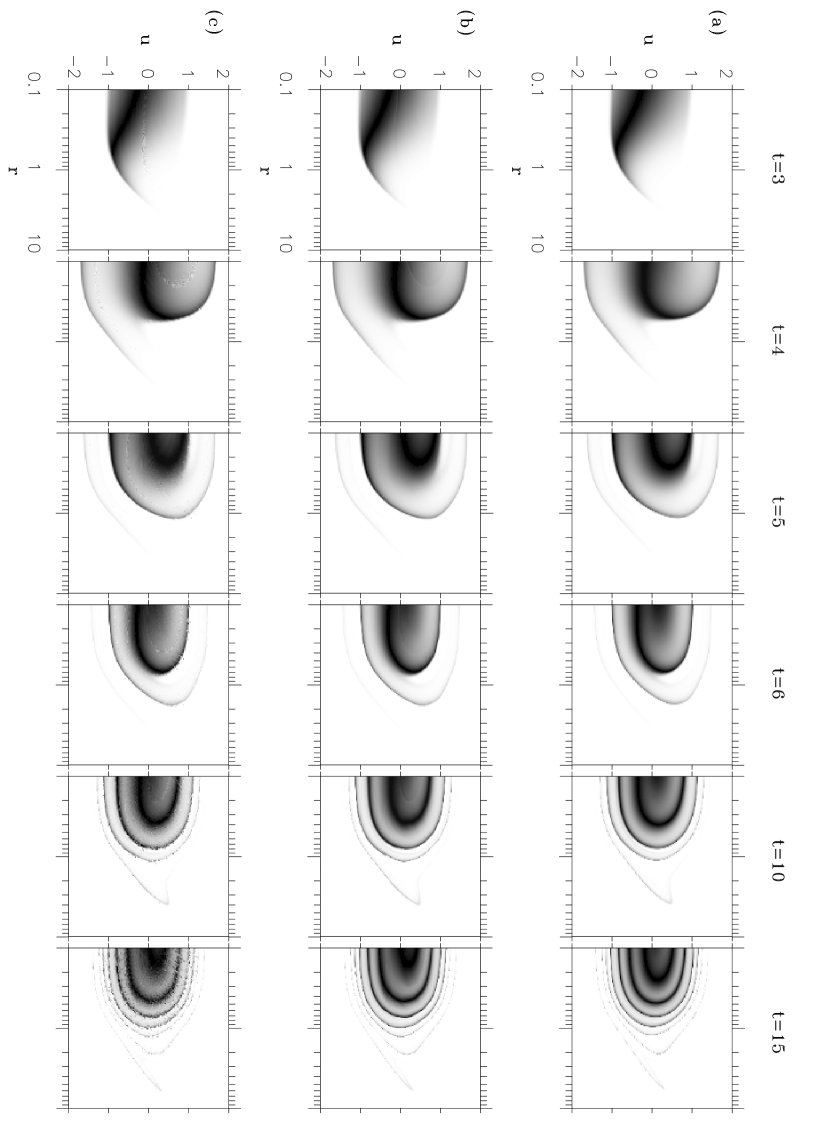
Figure 1: Phase-space evolution for the collapse of a uniform-density sphere on a $j=0.00068$ plane derived from the collisionless Boltzmann simulation (a), reproduced with the CB basis set (b), and with the HO basis set (c). The initial virial ratio is 1/2. The ordinate is the radial velocity, and the abscissa is the radius in a logarithmic scale.

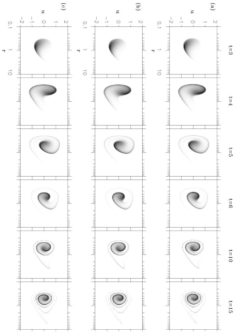
Figure 2: Same as in Fig. 1, but on a $j=0.329$ plane.

We show in Figures 1 and 2 the phase-space evolution reproduced with the CB and HO basis sets, along with that derived from the collisionless Boltzmann simulation. The detailed description of the collapse, beginning from uniform contraction through violent relaxation to phase mixing, is given by Fujiwara (1983a). It can be noticed that the evolution is essentially the same between the two SCF simulations, except for a ragged structure appearing on a $j=0.00068$ plane for the HO basis set. The origin of this unfavorable structure is discussed in the next section. On the other hand, a rough comparison in Figure 1 reveals that the phase-space evolution proceeds similarly in an essential sense between the phase-space solver and the SCF method with the CB basis set. However, a closer look reveals the difference which started to become noticeable at $t=6$, though the subsequent evolution did not deviate substantially between the two methods. In contrast to the evolution for the small value of the angular momentum, Figure 2 which represents phase space on a somewhat large angular-momentum plane demonstrates that there is no practical difference in phase-space evolution between the two methods, even when the HO basis set was used in the SCF simulation. In spite of the existing difference found in Figure 1, these figures manifest that the method of reproducing phase space proposed in this paper is competitive with that of directly integrating the collisionless Boltzmann equation as far as spherically symmetric systems are concerned.

Figure 1 indicates that the choice of basis sets affects the degree of the reproduction quality on small angular-momentum planes, that is, for the regions dominated by the stars passing close to the center. Clearly, the CB basis set is more suitable for reproducing phase space on every angular-momentum plane than the HO basis set. Nevertheless, we can understand from the same figure that the ragged structure resulting from the HO basis set will have no serious effects on the low order moments of the DF such as the density and velocity dispersions when such moments are evaluated directly from N particle distributions, because the velocity spread does not differ considerably between the two basis sets even on such small angular-momentum planes. In fact, this claim has already been demonstrated by HH who showed the excellent agreement in density and velocity dispersion profiles calculated from simulation particles though they used cooled Plummer models.

3.3 Distribution Function at a Relaxed State

The reproduction of the DF is another important aspect of the phase-space approach to collisionless dynamics. As argued by Fujiwara (1983a), incompleteness of violent relaxation leads to a degenerate DF in the core. Though Fujiwara (1983a) assumed spherical symmetry, May & van Albada (1984), using their expansion code, showed that the phase-space density in the core did not decrease substantially from its initial value for the three-dimensional collapse. Unfortunately, they estimated the phase-space density only in the mean sense like $\rho_{\rm c}/\sigma_{\rm c}^{3}$, where $\rho_{\rm c}$ and $\sigma_{\rm c}$ are the density and velocity dispersion in the core, respectively. We then demonstrate that our reproduction method can yield the DF itself.

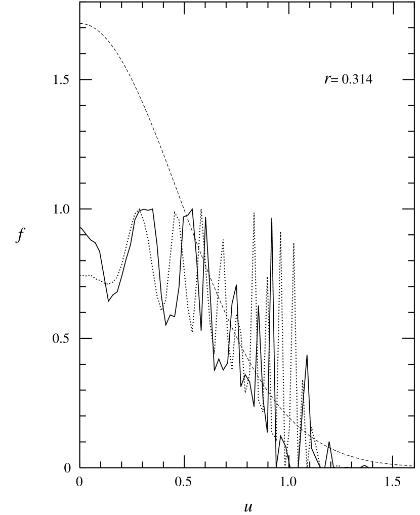
Figure 3: Distribution functions $f=f(r,u,j=0)$ in the core ($r=0.314$) for a relaxed state ($t=50$) of the uniform-density sphere, normalized by the initial maximum value of $(3M/4\pi R_{0}^{3})(2\pi\sigma_{0}^{2})^{-3/2}$, as a function of $u$. The solid line shows the DF reproduced with the CB basis set and the dotted line the DF derived from the collisionless Boltzmann simulation. The dashed curve represents a Maxwellian distribution function constructed with the density, $\rho(r)$, and the velocity dispersion, $\sigma^{2}$, at $t=50$ such that $f=\rho(r)(2\pi\sigma^{2})^{-3/2}{\rm exp}(-u^{2}/2\sigma^{2})$ with $\sigma^{2}=(\langle u^{2}\rangle+\langle j^{2}/r^{2}\rangle)/3$, normalized by $(3M/4\pi R_{0}^{3})(2\pi\sigma_{0}^{2})^{-3/2}$.

In Figure 3, $f(r,u,0)$ in the core ($r=0.314$) at a relaxed state ($t=50$) is presented for the SCF simulation with the CB basis set and the collisionless Boltzmann simulation, which corresponds to Figure 6 of Fujiwara (1983a). We show only the $u>0$ part of the DF because of its practical symmetry about $u$. We further mention that $f(r,0,j)$ in the core is very similar to $f(r,u,0)$, as shown by Fujiwara (1983a). Then, it can be noticed that the DF reproduced with our method is in good agreement with that derived from the phase-space method. In addition, the relaxed core is evidently degenerate because the values of the DF normalized by the maximum value of the initial DF are close to the unity for small values of $u$. To make clear the degeneracy, we have added a Maxwellian curve constructed from the density and velocity dispersions at $t=50$. This finding has already been pointed out by Fujiwara (1983a) who gave a possible mechanism of this degeneracy. The fluctuating behavior of the DFs reflects smaller and smaller structures generated from phase mixing with time, as stated by Lynden-Bell (1967). Figure 1 is also helpful to understand this behavior.

4 DISCUSSION

We argue the origin of the ragged structure appearing in the reproduced phase space with the HO basis set. Its lowest order member of the potential basis functions is reduced to the Hernquist model (Hernquist 1990):

$$\Phi_{000}^{\rm HO}(r)=-\frac{1}{1+r},$$ ()

in a dimensionless system of units. This potential generates the nonzero radial force, $f_{r}$, at the center: $f_{r}(0)=-1$. In reality, the force should converge to zero as $r\rightarrow 0$. Thus, the stars suffer fictitious forces when passing close to the center, so that their orbits are greatly displaced from the true orbits. This effect then emerges, as shown in Figure 1(c), as a ragged structure on small angular-momentum planes where stars orbiting close to the center are dominant. Of course, raggedness can be mitigated by choosing a smaller time step. In fact, with $\Delta t=0.0125$ and the other parameters intact, we recovered smoother phase plots than those shown in Figure 1(c) (not presented here), but we have found that there still remains raggedness. As a result, for small values of the angular momentum, we need much more computational cost to attain a smooth representation of phase space with the HO basis set than with the CB basis set. However, the nonvanishing force at the center no longer affects the orbits which avoid approaching the center closely. Therefore, we can find no unusual feature in the reproduced phase space of Figure 2(c) even with the HO basis set. On the other hand, since the zeroth order term of the potential basis functions for the CB basis set is the Plummer model (Plummer 1911; Binney & Tremaine 1987) given by

$$\Phi_{000}^{\rm CB}(r)=-\frac{1}{(1+r^{2})^{1/2}},$$ ()

the resulting force converges to zero as $r\rightarrow 0$. Consequently, the reproduced phase space with the CB basis set is a smooth distribution of phase particles.

We should point out that the phase-space solver used here also has a difficulty in following phase-space evolution for small values of the angular momentum. Since we set up a reflection wall at $R_{\rm min}$, the stars which have reached the region within $R_{\rm min}$ from outside are forced to be moved outside of $R_{\rm min}$ almost instantaneously with the sign of the radial velocity reversed. This means that the phase-space evolution on small angular-momentum planes proceeds faster than real, each time the stars traverse the reflection wall from outside, by approximately the crossing time of $2R_{\rm min}/U$, where $U$ is the typical radial velocity at $R_{\rm min}$. Indeed, when we adopted $R_{\rm min}=0.1$, we found that phase particles in the collisionless Boltzmann simulation were wound up many more times than those in the SCF simulations on a $j=0.00068$ plane because of the effect just mentioned. However, the phase-space evolution with $R_{\rm min}=0.005$ no longer showed any difference from that with $R_{\rm min}=0.01$.

Figure 4: Time evolution of radial forces, $f(r)$, for the uniform-density sphere as a function of radius. The solid lines are obtained with the CB basis set, the dashed lines with the HO basis set, and the dotted lines from the collisionless Boltzmann simulation.

On the other hand, SCF methods inherently have relaxation effects similar to those of the softening length as pointed out by Hernquist & Barnes (1990), so that the phase-space evolution obtained with the SCF method would not necessarily reproduce the true evolution. In this way, it is difficult to evaluate the numerical accuracy of phase-space evolution for the collisionless Boltzmann and SCF simulations. One measure for the accuracy may be to compare the evolving radial forces between the two methods. Then, we present in Figure 4 the radial forces at various times. We can notice from this figure that the forces expanded with the CB basis set are in good agreement with those from the collisionless Boltzmann simulation though there is a slight difference around the minimum values, which could come from the smoothing effects caused by the finite expansion terms in the SCF code. As compared to the CB basis set, the HO basis set gives a poor representation of the radial forces at small radii. In particular, within $r\sim 0.1$, the forces expanded with the HO basis set deviate appreciably from those with the CB basis set and become even positive around $R_{\rm min}=0.01$ except at $t=4$. Thus, we may understand again why the ragged structure appeared on a small angular-momentum plane when we used the HO basis set. Owning to the reflection wall within which there is no mass, the forces at $R_{\rm min}$ become exactly zero for the collisionless Boltzmann simulation. In this sense, the forces obtained with the CB basis set are more faithful to the real ones than those with the phase-space solver.

In addition to the phase-space evolution, the reproduced DF with the SCF technique is in good agreement with that using the phase-space solver, as shown in Figure 3. Besides, the reproduced DF is considered the fine-grained DF because our computation method of the DF suffers no coarse-graining. Since our reproduction method is easily applied to stellar systems with no special symmetries, we will be able to precisely study the degree of the degeneracy of the relaxed cores for three-dimensional collapses. In order to extend our method to general configurations, we again only save the expansion coefficients, $A_{nlm}$, at each time step to trace the orbits of stars backward to $t=0$. Of course, the quantum numbers, $l$ and $m$, have nonzero terms in this case. Although the extension of our method is quite straightforward, the development of smaller and smaller structures in phase space with time will force us to sample a large number of orbits for the accurate reproduction of the DF.

Since the success of the reproduction method proposed in this paper depends on the computation accuracy of individual orbits, a successful representation of the phase-space evolution, as demonstrated here, implies that the SCF technique enables us to compute the orbits of stars very close to the true orbits except for those passing near the center of the system. Therefore, the classification of orbit families like that done by van Albada (1987) can be made more reliably with the SCF method than with conventional N-body methods. In particular, SCF algorithms are well-suited for parallelized computer architectures (Hernquist & Ostriker 1992; Hernquist, Sigurdsson, & Bryan 1995), so that they can suppress discreteness noise by employing $N\gtrsim 10^{6}$. These algorithms will thus make feasible the orbit classification with sufficiently high accuracy. Furthermore, an algorithm, originally noticed by Merritt (1996) and recently realized by Weinberg (1996), for optimally choosing the maximum order term in the expansions such as $n_{\rm max}$ will be useful to give closer force fields to the exact ones.

5 CONCLUSIONS

We have demonstrated that the phase-space evolution for the collapse of a uniform-density sphere can be reproduced even using a particle method on the basis of Liouville’s theorem and with recourse to the SCF approach though spherical symmetry is assumed. Fortunately, our reproduction method is applicable to the systems with no special symmetries in contrast to the phase-space method whose application is restricted to the systems with some kind of symmetry due to memory limitations of presently available computers. The application of the present method to general aspherical systems is straightforward and can be realized only by saving the expansion coefficients, $A_{nlm}$, at each time step, though the computational cost increases in an SCF run and the orbit tracing because of the additional terms in the angular expansions. Therefore, we could no longer need to depend on collisionless Boltzmann simulations in order to access phase space, at least on such problems as the stability and collapse of the stellar systems having no symmetry.

For a good construction of phase space, we should choose such a basis set in the SCF code that the expanded forces converge to zero as $r\rightarrow 0$. If we use a basis set which gives rise to nonzero forces as $r\rightarrow 0$, the reproduced phase space will show a ragged structure for small values of the angular momentum. In this respect, the CB basis set which has no unusual characters in force is more suitable to the reproduction of phase space than the HO basis set whose expanded forces become nonzero at the center. However, the difference in the reproduced phase space resulting from the two basis sets disappears if somewhat large values of the angular momentum are chosen to plot phase particles.

We can also construct the DF itself with the SCF technique, which is found to be in good agreement with that obtained from the collisionless Boltzmann simulation. The reproduced DF is considered the fine-grained DF because of no coarse-graining included with our method. In addition, the present method for constructing the DF can be used to examine the degree of the degeneracy of the relaxed core for aspherical collapses of stellar systems.

The success of our reproduction method means that the individual orbits of stars are computed accurately. Thus, SCF algorithms can apply to the classification of orbit families to understand the kinematic properties of galaxies. Since the SCF method can employ a sufficiently large number of particles owning to its perfectly scalable nature, the orbit classification will be made with high accuracy by greatly reducing discreteness noise.

References

- (1)
- (2) Barnes, J., Goodman, J., & Hut, P. 1986, ApJ, 300, 112
- (3) Binney, J., & Tremaine, S. 1987, Galactic Dynamics (Princeton: Princeton Univ. Press)
- (4) Burkert, A. 1990, MNRAS, 247, 152
- (5) Cheng, C. Z., & Knorr, G. 1976, J.Comput.Phys., 22, 330
- (6) Clutton-Brock, M. 1972, Ap&SS, 16, 101
- (7) Clutton-Brock, M. 1973, Ap&SS, 23, 55 (CB)
- (8) Earn, D. J. D., & Sellwood, J. A. 1995, ApJ, 451, 533
- (9) Fujiwara, T. 1981, PASJ, 33, 531
- (10) Fujiwara, T. 1983a, PASJ, 35, 547
- (11) Fujiwara, T. 1983b, Prog.Theor.Phys., 70, 603
- (12) Hénon, M. 1973, A&A, 24, 229
- (13) Hernquist, L. 1990, ApJ, 356, 359
- (14) Hernquist, L., & Barnes, J. E. 1990, ApJ, 349, 562
- (15) Hernquist, L., & Ostriker, J. P. 1992, ApJ, 386, 375 (HO)
- (16) Hernquist, L., Sigurdsson, S., & Bryan, G. L. 1995, ApJ, 446, 717
- (17) Hernquist, L., Spergel, D. N., & Heyl, J. S. 1993, ApJ, 416, 415
- (18) Hernquist, L., & Weinberg, M. D. 1992, ApJ, 400, 80
- (19) Hoffman, Y., Shlosman, I., & Shaviv, G. 1979, MNRAS, 189, 737
- (20) Hohl, F. 1971, ApJ, 168, 343
- (21) Hozumi, S., Fujiwara, T., & Kan-ya, Y. 1996, PASJ, 48, 503
- (22) Hozumi, S., & Hernquist, L. 1995, ApJ, 440, 60 (HH)
- (23) Londrillo, P., Messina, A., & Stiavelli, M. 1991, MNRAS, 250, 54
- (24) Lynden-Bell, D. 1967, MNRAS, 136, 101
- (25) May, A., & van Albada, T. S. 1984, MNRAS, 209, 15
- (26) Merritt, D. 1996, AJ, 111, 2462
- (27) Min, K. W., & Choi, C. S. 1989, MNRAS, 238, 253
- (28) Mineau, P., Feix, M. R., & Rouet, J. L. 1990, A&A, 228, 344
- (29) Nishida, M. T. 1986, ApJ, 302, 611
- (30) Nishida, M. T., Watanabe, Y., Fujiwara, T., & Kato, S. 1984, PASJ, 36, 27
- (31) Nishida, M. T., Yoshizawa, M., Watanabe, Y., Inagaki, S., & Kato, S. 1981, PASJ, 33, 567
- (32) Ostriker, J. P., & Peebles, P. J. E. 1973, ApJ, 186, 467
- (33) Plummer, H. C. 1911, MNRAS, 71, 460
- (34) Press, W. H., Flannery, B. P., Teukolsky, S. A., & Vetterling, W. T. 1986, Numerical Recipes: The Art of Scientific Computing (Cambridge: Cambridge Univ. Press)
- (35) Rasio, F. A., Shapiro, S. L., & Teukolsky, S. A. 1989, ApJ, 344, 146
- (36) Sellwood, J. A. 1983, J.Comput.Phys., 50, 337
- (37) Shlosman, I., Hoffman, Y., & Shaviv, G. 1979, MNRAS, 189, 723
- (38) van Albada, T. S. 1987, in IAU Symp. 127, Structure and Dynamics of Elliptical Galaxies, ed. P. T. de Zeeuw (Dordrecht: Reidel), 291
- (39) Watanabe, Y., Inagaki, S., Nishida, M. T., Tanaka, Y. D., & Kato, S. 1981, PASJ, 33, 541
- (40) Weinberg, M. D. 1996, ApJ, 470, 715
- (41) White, R. L. 1986, in The Use of Supercomputers in Stellar Dynamics, ed. P. Hut & S. McMillan (Berlin: Springer), 167