First Structure Formation:
I. Primordial Star Forming Regions in hierarchical models.

Abstract

We investigate the possibility of very early formation of primordial star clusters from high–$\sigma$ perturbations in cold dark matter dominated structure formation scenarios. For this we have developed a powerful 2–level hierarchical cosmological code with a realistic and robust treatment of multi–species primordial gas chemistry, paying special attention to the formation and destruction of H₂ molecules, non–equilibrium ionization, and cooling processes. We performed 3–D simulations at small scales and at high redshifts and find that, analogous to simulations of large scale structure, a complex system of filaments, sheets, and spherical knots at the intersections of filaments form. On the mass scales covered by our simulations ($5\times 10^{5}-1\times 10^{9}\ M_{\odot}$) that collapse at redshifts $z>25$, we find that only at the spherical knots can enough H₂ be formed ($n_{H_{2}}/n_{H}\lower 2.15277pt\hbox{$\;\buildrel>\over{\sim}\;$}5\times 10^{-4}$) to cool the gas appreciably. Quantities such as the time dependence of the formation of H₂ molecules, the final H₂ fraction, and central densities from the simulations are compared to the theoretical predictions of Abel (1995) and Tegmark et al. (1997) and found to agree remarkably well. Comparing the 3–D results to an isobaric collapse model we further discuss the possible implications of the extensive merging of small structure that is inherent in hierarchical models. Typically only 5–8% percent of the total baryonic mass in the collapsing structures is found to cool significanlty. Assuming the Padoan (1995) model for star formation our results would predict the first stellar systems to be as small as $\sim 30\ M_{\odot}$. Some implications for primordial globular cluster formation scenarios are also discussed.

1 INTRODUCTION

Our primary interest is to study and identify the physics responsible for the formation of the first star in the universe. If the models put forward in previous investigations are correct, this is a very well defined problem because, for a given cosmogony, the thermodynamic properties, baryon content, and chemical composition are specified for the entire universe at high redshifts, at least in a statistical sense. Furthermore, the dominant physical laws are readily identified with the general theory of relativity describing the evolution of the background space–time geometry and particle geodesics, the Euler equations governing the motion of the baryonic fluid(s) in an expanding universe, and the primordial kinetic rate equations determining the chemical processes. Hence, at least in principal, given accurate numerical methods, one can directly simulate the formation of the first star in the universe. In practice, however, it turns out that the dynamical range required is beyond what current state–of–the–art numerical methods and super–computers can achieve. Nevertheless, it is worth stressing that the study of primordial star formation can yield stringent theoretical constraints on current cosmogonies. In fact it can even discard theories of structure formation if it is found that star formation is predicted to occur too late to explain the observed high redshift universe, such as the metal absorption lines present in quasar spectra at high redshifts.

Models for structure formation are based on the growth of small primordial density fluctuations by gravitational instabilities on a homogeneously expanding background universe. In all scenarios, the minimum mass scales to separate from the Hubble flow and begin collapsing are the smallest ones which survived damping until after the recombination epoch. Depending on the nature of the dark matter and whether the primordial fluctuations were adiabatic or isothermal, this mass scale could be as small as one solar mass (very heavy cold dark matter (CDM) particles) or as high as $\lower 2.15277pt\hbox{$\;\buildrel>\over{\sim}\;$}10^{13}M_{\odot}$ (HDM scenarios). In CDM cosmogonies, the fluctuation spectrum at small wavelengths has only a logarithmic dependence for mass scales smaller than $\sim 10^{8}M_{\odot}$, which indicates that all small scale fluctuations in this model collapse nearly simultaneously in time. This leads to very complex dynamics during the formation of these structures. Furthermore, the cooling in these fluctuations is dominated by the rotational/vibrational modes of hydrogen molecules that were able to form using the non–equilibrium abundance of free electrons left over from recombination and the ones produced by strong shock waves as catalysts (Saslaw & Zipoy, 1967; Couchman & Rees, 1986; Tegmark et al. 1997).

Couchman & Rees (1986) have argued that the first structures to collapse might have substantial influence on the subsequent thermal evolution of the intergalactic medium due to the radiation they emit as well as supernova driven winds. Haiman et al. (1997) have argued that the fragmentation of the first collapsed objects into stars can lead to the photoionization of the IGM and raise its temperature to $\sim 10^{4}$ K, and the Jeans mass to $M_{J}\gg 10^{5}~{}M_{\odot}$. Such an ionizing background can have a negative feedback effect on the molecular hydrogen fraction since H₂ can be destroyed by photons in its Lyman–Werner Bands which are below the Lyman limit. Accounting for self–shielding, Haiman et al. (1997) demonstrate that H₂ molecules inside virialized clouds are easily destroyed before the universe fully reionizes. The appearance of the first UV sources will thus suppress the H₂ abundance in primordial structures and prevent the post–virialization collapse. H₂ cooling is then also suppressed, even in massive objects, before the UV radiation photoionizes the entire IGM. The only clouds that are able to fragment into new stars have $T_{vir}=10^{4}$ K and nonlinear mass scales above the new Jeans mass $M>10^{8}(1+z_{vir}/10)^{-3/2}~{}M_{\odot}$. These conclusions will hold for structures that are collapsing after a significant UV background flux has been established. However, if structures collapse and cool to number densities $\lower 2.15277pt\hbox{$\;\buildrel>\over{\sim}\;$}1{\rm\ cm}^{-3}$ with neutral hydrogen column densities $\lower 2.15277pt\hbox{$\;\buildrel>\over{\sim}\;$}10^{18}{\rm\ cm}^{-2}$ before the onset of the UV flux, they are able to survive quite strong UV fluxes ($\lower 2.15277pt\hbox{$\;\buildrel>\over{\sim}\;$}10^{-22}{\rm\ erg}{\rm\ cm}^{-2}{\rm\ s}^{-1}$) (Haiman et al. 1996a; Abel & Mo 1997). Hence to know what structures will really be destroyed by the UV background, one first has to answer a crucial question: How long does it take to form the first stars in the universe?.

The pioneering studies on primordial star formation (i.e. Hutchins 1976; Palla et al. 1983) explored various aspects of the microphysical processes during protostellar collapse, the minimum attainable Jeans mass, and the accretion stage of primordial star formation. However, the time scale for the formation of a primordial star could not yet be determined due to the complexity and interactions of the hydro–dynamical, chemical, and radiative processes. The typically high computational requirements to solve the chemical rate equations alone have forced many previous studies to use the steady state shock assumption, or a spherical collapse model which formulate the problem without any spatial dimension. Only recently Bodenheimer et al. (1986) and Haiman et al. (1996b) were able to address the problem with spherically symmetric 1–D hydrodynamical calculations, including the non–equilibrium chemistry and cooling processes.

We have been able to develop numerical methods (Anninos, Zhang, Abel, & Norman 1997a) and an accurate chemistry and cooling model (Abel, Anninos, Zhang, & Norman 1997) that allow us to study the problem in three dimensions without imposing an equilibrium or other simplifying assumptions. Recently Gnedin and Ostriker (1997) have also developed a similar method allowing to model the non–equilibirum chemistry in multi–dimensional, hydrodynamical calculations. Here we use our code to study the origin of the first structures in the universe formed in the standard cold dark matter scenario (SCDM). Although the SCDM model fails to explain the observed large scale structure, it is still the prime example for any hierarchical clustering scenario and matches the observations of small scale systems remarkably well (see Zhang, Anninos & Norman 1995, and references therein).

This paper complements the first reported result from this work presented in Zhang et al. (1996). In section 2 we introduce an analytical description of small scale structure collapse based on the simplified studies of Abel (1995) and Tegmark et al. (1997). Section 3 discusses our numerical methods and presents and motivates our simulation parameters. In section 4 we show results from our 3–D investigations that illustrate the morphology of the first primordial star forming regions as well as comparing these results with the analytical picture outlined in section 2. We find remarkable agreement with the rough estimates of both Abel (1995) and Tegmark et al. (1997). We summarize our findings and comment on primordial Globular Cluster formation scenarios and models of primordial star formation in section 5.

2 Analytical Considerations for Small Scale Structure Collapse

2.1 The Density at Collapse

For the collapse of structures where the initial gas pressure is dynamically important, a simple estimate of the density at collapse is derived by solving the equations of hydrostatic equilibrium (Sunyaev & Zel’dovich 1972; Tegmark et al. 1997). Defining the virial temperature $T_{vir}$ through $3kT_{vir}/2=-m_{p}\Phi/2$, where $\Phi$ is the gravitational potential, the density contrast $\delta$ can be written as

$$\left(1+\delta\right)=\frac{\rho}{\rho_{B}}=\left(1+\frac{6}{5}\frac{T_{vir}}{T_{B}}\right)^{3/2},$$ (1)

where $T_{B}$ and $\rho_{B}$ denote the background temperature and density, respectively. The morphological characteristics of the object described by equation equation (1) is determined by the gravitational potential $\Phi$. The factor $1/2$ on the right hand side of the definition of $T_{vir}$ is chosen to reproduce the canonical definition of $3kT_{vir}/2=m_{p}v^{2}/2$ for a virialized spherical system with velocity dispersion $v$. The analysis of a spherical collapse model for structures where the initial gas pressure is not important gives for the overdensity at virialization $\delta=18\pi^{2}$ (Gunn and Gott 1972). Hence equation (1) should only be applicable as long as $\delta\lower 2.15277pt\hbox{$\;\buildrel<\over{\sim}\;$}18\pi^{2}$. Furthermore the assumption of hydrostatic equilibrium, which we used to derive equation (1), can only hold for structures with infall (virial) velocities that are small compared to the sound speed of the gas; meaning that no virialization shock will form. This is true for spherical objects with masses $\lower 2.15277pt\hbox{$\;\buildrel<\over{\sim}\;$}100\ M_{\odot}h^{-1}\Omega_{0}^{-0.5}(1+z_{coll})^{3/2}$, which is in reasonable agreement with the condition $\delta\lower 2.15277pt\hbox{$\;\buildrel<\over{\sim}\;$}18\pi^{2}$.

The matter temperature of the background universe decouples thermally from the radiation at $z\sim 200$ and evolves adiabatically ($TV^{\gamma-1}=const.$) afterwards. Hence we can write

$$T_{B}=135{\rm\ K}\left(\frac{1+z}{100}\right)^{2},$$ (2)

with which we find for the density at collapse,

$$n_{coll}=\left\{\begin{array}[]{ll}1{\rm\ cm}^{-3}\left(\frac{T_{vir}}{400{\rm\ K}}\right)^{3/2}\left(\frac{\Omega_{B}h^{2}}{0.025}\right),&\ \ \ {\rm for\ \ }\frac{T_{vir}}{400{\rm\ K}}<\left(\frac{1+z}{30}\right)^{2}\\ 1{\rm\ cm}^{-3}\left(\frac{1+z}{30}\right)^{2}\left(\frac{\Omega_{B}h^{2}}{0.025}\right),&\ \ \ {\rm otherwise.}\end{array}\right.$$ (5)

This suggests that, for the smallest structures, the typical density at collapse does not depend on the collapsing redshift, and that the chemical and cooling behavior for these structures will therefore be the same for any collapse redshift. However, the above analysis is certainly oversimplified in the sense that it does not include a detailed treatment of the dark matter potential in which the baryons will fall.

2.2 Molecular Chemistry and Cooling

Molecular hydrogen can not be destroyed efficiently in primordial gas at low temperatures ($<$ few $\times 10^{3}$K) unless there is a radiation flux higher than $\sim 3\times 10^{-26}{\rm\ erg}{\rm\ cm}^{-2}{\rm\ s}^{-1}$ in the Lyman Werner Bands. Once self–shielding is important even higher fluxes would be needed. Furthermore only two H₂ producing gas phase reactions operate on time–scales less than the Hubble time: the charge exchange reaction

$$\rm H_{2}^{+}\ \ \ +\ \ \ H\ \ \ \rightarrow\ \ \ H_{2}\ \ \ +\ \ \ H^{+},$$ (6)

and the dissociative attachment reaction

$$\rm H^{-}\ \ \ +\ \ \ H\ \ \ \rightarrow\ \ \ H_{2}\ \ \ +\ \ \ e^{-}.$$ (7)

The H₂ abundance will thus be determined by the H${}_{2}^{+}$ and H^- abundances. However, one typically finds that the H${}_{2}^{+}$ equilibrium abundance is much lower than that of H^- ($k_{9}\ll k_{7}$ in the notation of Abel et al. 1997a) and additionally that the rate coefficient of reaction (6) is about $2.4$ times less than reaction (7). Hence the H₂ formation is dominated mostly by reaction (7).

In the absence of an external UV background at gas temperatures below 6000K, one can integrate the rate equations for the free electron and the molecular hydrogen fraction to find the time evolution of the H₂ fraction during the collapse of primordial gas clouds (see Abel 1995 and Tegmark et al. 1997)

$$f_{H_{2}}(t) = f_{H_{2}}(t=0)+\frac{k_{PA}}{k_{rec}}\ln(x_{0}n_{H}k_{rec}t+1)$$ (8)

$$= f_{H_{2}}(t=0)+1.0\times 10^{-8}T_{vir}^{1.53}\ln(t/t_{rec}+1),$$

where $k_{PA}$, $k_{rec}$, $t_{rec}$, $x_{0}$, and $n_{H}$ are the rate coefficients of photo–attachment of H^- and recombination to neutral hydrogen in ${\rm\ cm}^{3}{\rm\ s}^{-1}$, the initial recombination timescale (see equation (9)), the initial ionized fraction, and the neutral hydrogen number density (in cm^-3), respectively. The production of H₂ therefore only depends logarithmically on time, and increases most rapidly within the first few initial recombination timescales so that it defines an H₂ formation timescale,

$$t_{rec}=\frac{1}{n_{H^{+}}k_{rec}}=5.0\times 10^{13}\left(\frac{n_{H}}{100{\rm cm}^{-3}}\right)^{-1}\left(\frac{x}{10^{-4}}\right)^{-1}\left(\frac{T}{1000{\rm K}}\right)^{0.65}\ \ {\rm s},$$ (9)

where $k_{rec}=1.8\times 10^{-10}T^{-0.65}{\rm\ cm}^{3}{\rm\ s}^{-1}$ is our own fit to the data of Ferland et al. (1992), which is accurate to within a few percent for temperatures below $10^{4}$K. A good estimate for the typical H₂ fraction is given by evaluating equation (8) at $t\sim 2t_{rec}$. The temperature dependence enters from the ratio of the recombination and H^- formation rates. A typical H₂ fraction of $n_{H2}/n\sim 10^{-3}$ is produced during the collapse of structures with virial temperatures greater than $10^{3}{\rm\ K}$. For temperatures higher than $6000{\rm\ K}$, the charge exchange with protons will efficiently destroy H₂, and equation (8) will not be applicable. However, during the collapse of clouds with such high virial temperatures, the final H₂ fraction will, nevertheless, be $f_{H_{2}}(T\sim 6000{\rm\ K})\sim 6\times 10^{-3}$ (see Abel et al. 1997a). Comparing equation (8) with the dynamical timescale for a spherical top–hat model, Tegmark et al. (1997) argued for a rule of thumb, stating: “A spherical primordial gas cloud will be able to undergo a stage of free-fall collapse if its H₂ fraction becomes $\lower 2.15277pt\hbox{$\;\buildrel>\over{\sim}\;$}5\times 10^{-4}$.”

2.3 Isobaric Collapse

It has been found by numerous authors (see e.g. Mac Low and Shull, 1986; Shapiro and Kang, 1987; Anninos & Norman, 1996, Abel et al.  1997b) that the postshock gas of a radiative shock originating in structure formation evolves under constant pressure ($\rho_{b}\times T\propto p=const$, where $\rho_{b}$, $T$ and $p$ are the density, temperature and pressure of the baryonic fluid). Although there is no reason to assume that isobaric evolution is also appropriate for spherical collapsing structures it is useful to compare our simulations to such simplified models. Constant pressure implies that the internal energy density of the gas, $e$, also remains constant (assuming an ideal gas for which $e=p/(\gamma-1)$). Differentiation of the isobaric condition yields the following form of the constant pressure condition

$$\frac{\delta\rho_{b}}{\rho_{b}}=-\frac{\delta T}{T}.$$ (10)

The temperature evolution equation is found using the energy conservation equation that neglects conduction, viscosity, and kinetic energy terms

$$\frac{du}{dt}=-\frac{p}{\rho_{b}^{2}}\frac{d\rho_{b}}{dt}+\frac{\Lambda}{\rho_{b}},$$ (11)

where $u=e/\rho_{b}$ is the energy per unit mass and $\Lambda=\dot{e}$ the cooling function of the gas. Inserting the isobaricity condition (10) into equation (11), we derive the following simple ordinary differential equation for the temperature evolution:

$$\frac{\dot{T}}{T}=\frac{\dot{e}(n,T)}{\gamma\ e(n,T)}\ \ \ \leftrightarrow\ \ \ \dot{T}=\frac{T}{\gamma\ t_{cool}(p_{0}/T,T)}.$$ (12)

Here we substituted the temperature for the density using $n=p_{0}/T$, where $p_{0}=T_{0}n_{0}$ is the initial pressure at collapse and $\gamma$ ($=5/3$ for an ideal gas) is the adiabatic index. The isobaricity condition ($nT=n_{vir}T_{vir}$ throughout the contraction) implies that the density at the final stages of the isobaric collapse will be $n\sim n_{vir}T_{vir}/50{\rm\ K}$ since H₂ cooling becomes inefficient at temperatures $\lower 2.15277pt\hbox{$\;\buildrel<\over{\sim}\;$}50{\rm\ K}$.

3 THE SIMULATIONS

A numerical code with high spatial and mass resolution is required to model both the collapse of sufficiently large scale structure and the microphysics of chemical reactions and radiative cooling which are important on the smaller scales. We can achieve high dynamical ranges with the two–level hierarchical three–dimensional code (HERCULES) that we have developed for cosmology (Anninos, Norman & Clarke 1994; Anninos, Zhang, Abel & Norman 1997). This code is designed to simulate structure formation in an expanding dark matter dominated universe with Newtonian gravity, multi–fluid hydrodynamics, radiative cooling, non–equilibrium chemistry and external radiation fields. It also utilizes nested grid methods for both the gas and dark matter particles to achieve higher resolution over a selected sub–domain of the coarser parent grid. At the small scales resolved by our calculations, it is important to track the different chemical species in order to model the chemistry and radiative cooling accurately. For this purpose we independently evolve the following nine species: neutral hydrogen H, ionized hydrogen H⁺, negative hydrogen ions H^-, hydrogen molecules H₂, ionized hydrogen molecules H${}_{2}^{+}$, neutral helium He, singly–ionized helium He⁺, doubly–ionized helium He⁺⁺, and free electrons $e^{-}$. The 28 most important chemical rate equations (including radiation processes) are solved in non–equilibrium for the abundances of each of the nine species. The rate coefficients used in the chemistry model are provided in Abel, Anninos, Zhang & Norman (1997a). We have also implemented a comprehensive model for the radiative cooling of the gas (Anninos, Zhang, Abel & Norman 1997) that includes atomic line excitation, recombination, collisional ionization, free–free transitions, molecular line excitations, and Compton scattering of the cosmic background radiation (CBR) by electrons.

We apply our code to high redshift pre–galactic structure formation and evolution, investigating specifically the collapse of the first high–$\sigma$ bound objects with baryonic masses in the range $10^{4}-10^{8}M_{\odot}$. Our model background spacetime is a flat ($\Omega_{0}=1$) cold dark matter dominated universe with Hubble constant $H_{0}=50$ km s^-1 Mpc^-1 and baryon fraction $\Omega_{B}=0.06$, consistent with the constraints from big–bang nucleosynthesis (Copi, Schramm & Turner 1995). The baryonic matter is composed of hydrogen and helium in cosmic abundance with a hydrogen mass fraction of 76% and ratio of specific heats $\gamma=5/3$. The data is initialized at redshift $z=100$ with matter perturbations derived from the Harrison–Zel’dovich power spectrum modulated with a transfer function appropriate for CDM adiabatic fluctuations and normalized to the cluster scale $\sigma_{8h^{-1}}=0.7$. Bertschinger’s (1994) constrained realization procedure is used to construct 3 and 4$\sigma$ fluctuations at the box center over a region of 1/5 the box length.

The chemical abundances are initialized according to the estimates provided by Anninos & Norman (1996). For the primary hydrogen and helium species, we use the residual ionization estimate of Peebles (1968, 1993):

$$\frac{n_{H^{+}}}{n_{H}}=2.4\times 10^{-4}~{}\Omega_{0}^{1/2}\frac{0.05}{h\Omega_{B}},$$ (13)

and assume negligible amounts of $n_{He^{+}}/n_{H}$ and $n_{He^{++}}/n_{H}$ ($\lesssim 10^{-14}$). The concentrations of the intermediaries H^- and H${}_{2}^{+}$, and hydrogen molecules are given by

$$\frac{n_{H^{-}}}{n_{H}} = 2\times 10^{-9}~{}T_{K}^{0.88}~{}\frac{n_{H^{+}}}{n_{H}}~{},$$ (14)

$$\frac{n_{H_{2}^{+}}}{n_{H}} = 3\times 10^{-14}~{}T_{K}^{1.8}~{}\frac{n_{H^{+}}}{n_{H}}~{},$$ (15)

$$\frac{n_{H_{2}}}{n_{H}} = 2\times 10^{-20}\frac{f_{H}\Omega_{0}^{3/2}}{h\Omega_{B}}(1+z_{o})^{5.1}~{},$$ (16)

where $T_{K}$ is the gas temperature in degrees Kelvin, and is set at the starting redshift by assuming an adiabatic expansion from $z=200$, the approximate redshift at which matter/radiation interactions are negligible (see equation (2)). Also, $f_{H}$ is the hydrogen mass fraction and $z_{o}=300$ is an estimate for the largest redshift at which H${}_{2}^{+}$ can form efficiently to produce hydrogen molecules without being photodissociated by the cosmic background radiation. For our model parameters ($f_{H}=0.76$, $\Omega_{0}=1$, $\Omega_{B}=0.06$ and $h=0.5$), we find $n_{H_{2}}/n_{H}=2.9\times 10^{-6}$. The neutral hydrogen and helium, and electron densities are then set by the following conservation equations:

$$\rho_{He}+\rho_{He^{+}}+\rho_{He^{++}}=\rho_{b}~{}(1-f_{H})~{},$$ (17)

$$\rho_{H}+\rho_{H^{+}}+\rho_{H^{-}}+\rho_{H_{2}^{+}}+\rho_{H_{2}}=\rho_{b}~{}f_{H}~{},$$ (18)

$$\rho_{H^{+}}-\rho_{H^{-}}+\frac{1}{2}\rho_{H_{2}^{+}}+\frac{1}{4}\rho_{He^{+}}+\frac{1}{2}\rho_{He^{++}}=m_{H}~{}n_{e}~{},$$ (19)

where $\rho_{i}$ are the densities of the $i$th species, $\rho_{b}$ the total baryonic density, $n_{e}$ the number density of free electrons, and $m_{H}$ the proton mass.

In this paper we present results from six different nested grid calculations. We investigate the effect of increasing the large scale power by varying the parent box size over $L=$ 128, 512 and 1024 kpc, and set up initial data for the collapse of both 3$\sigma$ and 4$\sigma$ fluctuations. The different box sizes act to parameterize the mass of the collapsing structures. The data from the sub grid (top grid) simulation of a $4\sigma$ peak within a box of size 512kpc is referred to as $4\sigma 512$S ($4\sigma 512$T). For a fixed mass scale, $\sigma$ effectively defines the redshift at which the structures begin to collapse. A box dimension of 1024 kpc is about the maximum we can set before losing the resolution in the sub grid needed to resolve the H₂ chemistry and cooling. We use $128^{3}$ cells to cover both the top and sub grids which, for the refinement factor of four used in all our simulations, results in an effective $512^{3}$ resolution over the sub grid domain. The spatial and mass resolutions of the parent and child grids are shown in Table 1 for each of the calculations.

Run Grid $L$ (kpc) $\Delta x$ (kpc) $M_{DM}$ ($M_{\odot}$) $M_{B}$ ($M_{\odot}$) $\Delta M_{DM}$ ($M_{\odot}$) $\Delta M_{B}$ ($M_{\odot}$) 3(4)$\sigma$1024T top 1024 8 $7.5\times 10^{10}$ $4.5\times 10^{9}$ $3.6\times 10^{4}$ $2.1\times 10^{3}$ 3(4)$\sigma$512T top 512 4 $9.3\times 10^{9}$ $5.6\times 10^{8}$ $4.4\times 10^{3}$ $2.7\times 10^{2}$ 3(4)$\sigma$128T top 128 1 $1.5\times 10^{8}$ $8.8\times 10^{6}$ $6.9\times 10^{1}$ $4.2\times 10^{0}$ 3(4)$\sigma$1024S sub 1024 2 $1.2\times 10^{9}$ $7.1\times 10^{7}$ $5.6\times 10^{2}$ $3.3\times 10^{1}$ 3(4)$\sigma$512S sub 512 1 $1.5\times 10^{8}$ $8.8\times 10^{6}$ $6.9\times 10^{1}$ $4.2\times 10^{0}$ 3(4)$\sigma$128S sub 128 0.25 $2.3\times 10^{6}$ $1.4\times 10^{5}$ $1.1\times 10^{0}$ $6.7\times 10^{-2}$

Table 1: Spatial and mass resolution of the different top and sub grid simulations. $L$ is the comoving box size of the top grid defining the longest wavelength perturbation, $\Delta x$ the comoving cell size in each computational box, $M_{DM}$ the total dark matter mass initially in each grid, $M_{B}$ the total baryonic mass, $\Delta M_{DM}$ the single dark matter particle mass, and $\Delta M_{B}$ the baryonic mass in a single cell at the start of the simulation at redshift $z=100$. The same parameters were used for both the 3 and 4$\sigma$ perturbation simulations. We employ the notation 4$\sigma$1024T, for example, to denote the top grid simulation of a $4\sigma$ peak in the 1024$Mpc$ box.

For comparison, we note that the mass resolution is much smaller than the Jeans mass in the background baryonic fluid, which varies from about $10^{6}M_{\odot}$ at $z=100$ to $\sim 10^{4}M_{\odot}$ at $z=10$.

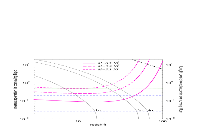
Figure 1: The solid lines labeled 1, 3, and $4\sigma$ depict the length scales of 1, 3, and $4\sigma$ peaks vs. their collapse redshift as predicted by linear theory. This assumes a Gaussian adiabatic CDM spectrum with $\sigma_{8}=0.7$, $\Omega_{0}=1$, and $h=0.5$, and a linear density contrast of $\delta_{c}=1.68$ at collapse. The thick solid, long dashed, and dashed lines depict the comoving mean separation of peaks with a mass of $6.2\times 10^{5}$, $3.9\times 10^{7}$, and $3.1\times 10^{8}\ M_{\odot}$, as predicted by the Press–Schechter formalism, respectively. These masses correspond to the three different perturbation wavelengths we have simulated: $25.6$, $102.4$, and $204.8{\rm\ kpc}$ (dashed horizontal lines). The dotted horizontal lines show our box sizes, $1024$, $512$, and $128$ comoving kpc. For reference, the Hubble horizon is shown as a dot–dashed line (in the upper right corner).

In Figure 1 we show the mean comoving separation, computed from the Press Schechter (1974) formalism, of the three different mass scales we have simulated. The solid, long dashed, and dashed lines correspond to a total collapsing mass of $6.2\times 10^{5}$, $3.9\times 10^{7}$, and $3.1\times 10^{8}\ M_{\odot}$ respectively. These masses correspond to perturbation wavelengths (dashed horizontal lines in Figure 1) of $25.6$, $102.4$, and $204.8{\rm\ kpc}$, respectively. On the same graph we also plot the perturbation wavelength vs. the redshift at which linear theory predicts its overdensity to be 1.68 (its collapse redshift) for $\sigma=1$, 3, and 4 peaks (solid downward sloping lines labeled $1\sigma$, $3\sigma$, and $4\sigma$). Our simulation box sizes are indicated by the horizontal dotted lines. We see that the $25.6{\rm\ kpc}$ perturbation of the $4\sigma 128$ ($3\sigma 128$) simulation is expected to collapse at a redshift $\sim 65$ ($\sim 50$). At this redshift the typical mean separation of such $6.2\times 10^{5}\ M_{\odot}$ objects is $\sim 700{\rm\ kpc}$ ($\sim 220{\rm\ kpc}$) which is $5.5$ ($1.7$) times greater than the simulation box size of $128{\rm\ kpc}$. For the larger box sizes (512 and $1024{\rm\ kpc}$), the mean separation of peaks is larger than the box at the collapse redshift by a factor of a few and about half the box size for smaller redshifts. Figure 1 also shows that at a redshift of $\sim 11$, $7$, and $5$ a ($1\sigma$) perturbation of 128, 512, and $1024{\rm\ kpc}$, corresponding to our box sizes, would go non–linear, respectively. Therefore, one cannot trust the simulation results for smaller redshifts. Although the mean separation of the simulated peaks is always within a factor of five of the box sizes, the use of periodic boundary conditions on these small scales will also limit the reliability of our results.

4 RESULTS

4.1 Morphology

In Figure 11 we show an evolution sequence of the logarithm of the dark matter and gas overdensities at four redshifts $z=$ 35, 22, 17, and 12. Five contour levels of $\log\rho/\overline{\rho}=(0.5,1,1.5,2,2.5)$ are displayed in the $x$–$y$ plane of the cube intersecting the maximum density peak. Each plot in the figure represents the data from the top grid evolution for the 3$\sigma$ collapse with the intermediate box size $L=512{\rm\ kpc}$ ($3\sigma 512$T). In the evolution sequence of the gas density one can see two originally distinct objects (at $z=35$) that merge later on. By redshift $z=22$, a well developed spherical structure of total mass $4\times 10^{7}~{}M_{\odot}$ forms at the intersection of several filaments, consistent with the prediction from linear theory that a 3$\sigma$ peak of mass $\sim 10^{7}~{}M_{\odot}$ will collapse at $z\sim 35$. The structure continues to grow by the further collapse of nearby particles and gas, and by the merging of smaller collapsed structures. The total mass of the bound structure grows to $1.3\times 10^{8}~{}M_{\odot}$, with baryonic mass $6.8\times 10^{6}~{}M_{\odot}$ by $z=12$. Figure 12 shows results analogous to those in Figure 11, but for the sub grid evolution. The enhanced resolution (a factor of four in length and 64 in mass) allows for more detailed and accurate studies of the collapsing structure. In fact, it is the enhanced resolution that allows the cooling flow to be resolved adequately. The top grid calculation does not have the resolution required to produce significant amounts of hydrogen molecules to cool the gas effectively. Also, in the sub grid data, a more complex network of filamentary structure is resolved due to the higher mass resolution. Evidently the filamentary structures observed in the gas appear also in the DM overdensity, consistent with the picture that the baryons fall into the potential well of the dark matter. In the gas overdensity (Figure 12) one observes how a distinct overdense region forms in the upper filament between redshifts 22 and 17, and merges then with the more massive central structure by $z=12$. It is evident that a significant amount of mass accretes onto the central object along the filaments.

Analogous to Figure 12, Figure 13 shows the evolution sequence for the gas temperature and molecular hydrogen number density fraction $n_{H2}/n_{H}$ on the sub grid. The contour levels are $\log T(eV)=-2.2,-2,-1.5,-1,-0.5$ and $\log n_{H2}/n_{H}=-5.05,-5,-4.5,-4,-3.5$. H₂ fractions exceeding the background value of $\sim 3\times 10^{-6}$ are found only in overdense regions along the filamentary structures, and predominantly at their intersections where the densities are highest. We find typical H₂ fractions of $\sim 10^{-5}$ along the filaments, and $\lower 2.15277pt\hbox{$\;\buildrel>\over{\sim}\;$}10^{-4}$ in the spherical overdense regions. Both of the spherical structures that are most evident in the gas contour plots of Figure 12, and merge between redshift 17 and 12, show H₂ fractions exceeding $3\times 10^{-4}$. By redshift $z=12$ the fraction of H₂ in the central structure increases to $9.1\times 10^{-4}$, which is enough to cool the gas to $0.21eV~{}(2390K)$ and to collapse the gas to a central density of $\sim 100{\rm\ cm}^{-3}$. Approximately 6% of the baryonic mass in the structure has cooled by $z=12$, so the collapsed and cooled structure is roughly of mass $4\times 10^{5}\ M_{\odot}$. We note that the merger event did not destroy any molecules in the merging structures (see also Figure 8 below).

4.2 Profile Plots

In the following we present radial profile plots which represent physical quantities averaged in spherical shells centered on the densest cell in the high resolution sub grid. All of these radially averaged quantities do not include the central zone.

Figure 2a shows the ratio of baryonic to total density for all of the $4\sigma$ runs vs. the distance from the center in comoving kpc. The horizontal line depicts the background (initial) value of $\Omega_{B}/\Omega=0.06$. Evidently the cooling at the center of the structure allows the baryons to contract, leading to an enhancement of baryons over the dark matter up to four times the background value. The radius at which the ratio of baryonic to total density starts to exceed $\Omega_{B}/\Omega=0.06$ coincides with the radius at which the molecular hydrogen fraction reaches $5\times 10^{-4}$. This value agrees well with the analytical model presented in section 2 Note that the virial shock is located at radii larger than where the deficit is found. Hence, it is the shocked gas that forms molecules, cool, and settles to the center of the structure yielding the baryonic to DM bias.

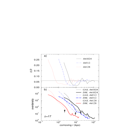
Figure 2: (a) Radial profile of the baryonic fraction for the $4\sigma$ runs. The horizontal solid line is the average baryonic fraction $\Omega_{b}=0.06$. (b) Radial profile of gas and dark matter overdensities for the $4\sigma$ runs. Note that the baryonic density increases substantially relative to that of the dark matter in the central core due to $H_{2}$ cooling. The arrows indicate the theoretical virial radii of the three different perturbation wavelengths we have simulated.

(see also Figure 8). The cooling gas flows from the outer region to the center causing the the deficit of baryons compared to the background value seen in Figure 2a.

The baryon enhancement at the center of the structures leads to sharp overdensity profiles as shown in Figure 2b. The radially averaged dark matter density profile shows a complex form with apparently four regimes of different slopes. Powerlaws that fit this radial dependence have an exponent $\lower 2.15277pt\hbox{$\;\buildrel<\over{\sim}\;$}-1$ at the central regions, then $\sim-2$, $-4$, and again $-2$ at the outer regions. The arrows in Figure 8 indicate the theoretical viral radii of collapsed spheres with intial wavelengths corresponding to the ones we have simulated ($r_{vir}=(l/2)(18\pi^{2})^{-1/3}$, where $l$ is the pertubration wavelength). Note that for the least massive halo the $r^{-4}$ feature is found just outside the virial radius, where for the others its partially ($4\sigma 512$) and completely ($4\sigma 1024$) within the virial radius. This is because we plot the profiles at redshift 17 at which only the smallest simulated structures is fully virialized. Generally we see the halo DM profiles within the virial radius to be isothermal ($\rho\propto r^{-2}$) over a wide range of radii. This shape is the typical behavior of the universal density profile proposed by Navarro, Frenk, and White (1996, NFW hereafter),

$$\rho(r)\propto\frac{1}{(r/r_{s})(1+r/r_{s})^{2},}$$ (20)

where $r_{s}$ is some characteristic radius. They showed this formula to fit DM haloes within the virial radius of the galaxies and clusters of galaxies found in their N–body simulations. Although Navarro et al. studied DM profiles for halos with masses $\sim 10^{12}\ M_{\odot}$, their results are similar to what we find in our simulated halos, which are approximately $10^{6}$ times smaller in mass. However, our DM profiles are somewhat sharper than the NFW profile making a future high resolution study desirable to test the applicability of the universal profile to DM halos on mass scales $\lower 2.15277pt\hbox{$\;\buildrel<\over{\sim}\;$}10^{8}\ M_{\odot}$ and clarify the “feedback” of the collapsing baryons on the DM density profile.

Figure 3 illustrates that the central regions of collapsing small scale structure can cool with molecules that are formed using free electrons that were left over from recombination as catalysts. It shows the radially averaged profiles for the fractional abundances of H₂ , H^- , H${}_{2}^{+}$ , and e^-, as well as the temperature for the $3\sigma 512$S data at $z=27$.

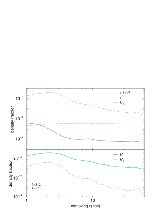
Figure 3: Profiles of temperature and several important species (H₂, H${}_{2}^{+}$, H^- and $e^{-}$) at $z=27$ for the $3\sigma 512S$ run. The depletion of H^- , H${}_{2}^{+}$ , and e^- in the H₂ forming and cooling region is evident. The virialization shock is not ionizing (yet) since the free electron fraction remains constant away from the central regions.

The molecular hydrogen formation is dominated by the H^- path, which is similar to the situation of strong shocks ($v_{s}\sim 100\,{\rm{km\,s^{-1}}}$) formed during the collapse of cosmological sheets (Anninos & Norman 1996, and Abel et al. 1997). This is clear from Figure 3 since the H^- abundance exceeds the H${}_{2}^{+}$ abundance by always more than an order of magnitude, and the fact that the dissociative attachment reaction of H^- to form H₂ is characterized by a rate coefficient that is two times greater than the charge exchange reaction of H${}_{2}^{+}$ with H (reactions (6) and (7)). The free electron abundance is decreased in the more dense and cooling center where the radiative recombination timescales are short. The weak shock is not capable of ionizing the primordial gas at this redshift. The decrease of the H^- abundance in the cooling layer is a result of the temperature decrease and the free electron depletion. Note that these results justify all the assumptions that entered the derivation of equation (8), further validating the analytical description given in section 2. Although the central parts of the structure formed hydrogen molecules solely from the residual free electrons as catalysts, at later redshifts the infalling material will be, at least partially, collisionally ionized by the stronger shock, allowing molecules to form on a faster timescale (see Figure 4). Furthermore, we can see that the minimal chemistry model proposed by Abel et al. (1997a) would be sufficient to study the effects of primordial gas chemistry for first structure formation.

4.3 Evolution

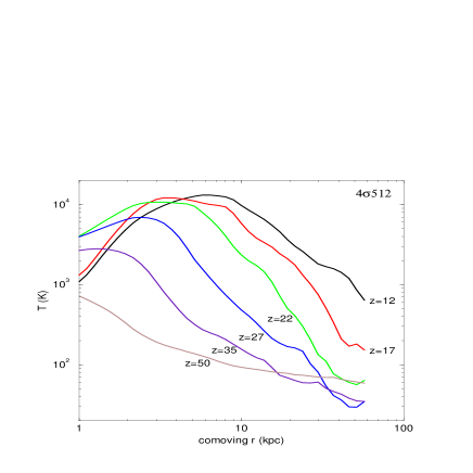
Figure 4: Radially averaged temperature profiles for the $4\sigma 512$S sub grid evolution. The adiabatic compression of the central regions is the dominant effect at redshift $z=50$. At $z\sim 35$, H₂ cooling dominates adiabatic heating in the central–most regions, and effectively cools the gas. At redshifts $\lower 2.15277pt\hbox{$\;\buildrel<\over{\sim}\;$}25$ the radially averaged temperature exceeds $10^{4}{\rm\ K}$ at a few comoving kpc from the center.

The temperature profiles for different redshifts of the $4\sigma 512$S box are shown in Figure 4. (The central temperatures can be read from Figure 7.) Clearly the virialization shock becomes stronger as more baryons collapse towards lower redshifts. It is interesting that for the small scale structures considered here that the central region never reaches temperatures above a few thousand Kelvin. For the $4\sigma 128$S run the maximum temperature in the center of the densest structure is only $\sim 900{\rm\ K}$ (see Figure 7). At $z=50$, the temperature profile shows a gentle increase towards the center caused by adiabatic compression with its maximum at the center. At $z=35$, the influence of radiative cooling causes the maximum temperature in the structure, which increases steadily through mass accretion, to be found away from the high density center core. At redshifts $z\lower 2.15277pt\hbox{$\;\buildrel<\over{\sim}\;$}22$, the radially averaged post–shock temperature exceeds $10^{4}{\rm\ K}$, and hence the gas becomes collisionally ionized, and more and more molecules form in the center to cool the gas to lower and lower temperatures.

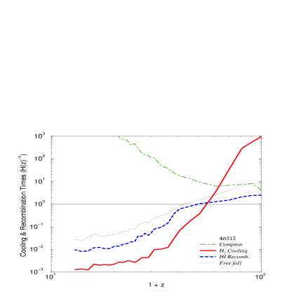
Figure 5: Cooling times in the densest cell found on the sub grid of the simulation $4\sigma 512$S, relative to the Hubble time $H^{-1}=H_{0}^{-1}(1+z)^{-3/2}$, for various physical processes, including Compton, and molecular hydrogen line cooling. Also shown are the hydrogen recombination and spherical free fall times.

Figure 5 shows some characteristic time scales normalized to the Hubble time ($H^{-1}=H_{0}^{-1}(1+z)^{-3/2}$, where $H_{0}$ is the present Hubble constant) of the most important physical processes in the densest cell of the collapsing structure in the $4\sigma 512$S simulation. The Bremsstrahlung and recombination cooling times exceed the expansion time scale by more than three orders of magnitude and are therefore not shown in the Figure. The hydrogen recombination time is already close to the Hubble time at $z=100$, allowing H₂ to form slowly. At redshift $z\approx 50$, the gas density and temperature grow to the levels that are more favorable for the creation of hydrogen molecules and the H₂ cooling time becomes shorter than the hydrogen recombination (equation (9)) and dynamical ($t_{dyn}=(3\pi/(32G\rho))^{1/2}=4.7\times 10^{7}n^{-1/2}{\rm\ years}$) times. The Compton cooling/heating exceeds the expansion time scale for all redshifts $\lower 2.15277pt\hbox{$\;\buildrel<\over{\sim}\;$}100$ and does not influence the collapse of the central regions. The reason that the H₂ cooling time is monotonically decreasing with redshift and does not start to increase again is due to the merging of small scale structures and, for the largest box sizes, an artifact of our limited numerical resolution as we will show in the following.

The decrease in temperature and increase in density at the cores results in an even greater decrease in the Jeans mass

$$M_{J}=\frac{\pi}{6}\rho\lambda_{J}^{3}=\frac{\pi}{6}\rho\left(\frac{\gamma\pi kT}{G\rho\mu m_{H}}\right)^{\frac{3}{2}}\approx 100T_{K}^{3/2}n_{B}^{-1/2}~{}M_{\odot},$$ (21)

as shown in Figure 6.

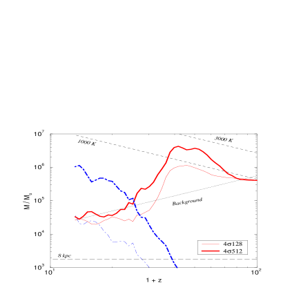
Figure 6: Evolution of the Jeans mass in the densest cell of the most massive structures in the $4\sigma 128$S and $4\sigma 512$S simulations (thin and thick solid lines). Also shown are the corresponding mass in the densest cell (thin and thick dot–dashed lines), the Jeans mass of the background baryonic density (dotted line), the initial baryonic mass in a single cell of the coarsest grid simulation (the parent 1024 kpc grid with a comoving cell size of 8 kpc, horizontal dashed line), and the Jeans mass for spherical collapse with virial temperatures of 1000 and 3000K (dashed lines labeled with 1000K and 3000K, respectively).

Here $n_{B}$ denotes the baryonic number density expresses in numbers of hydrogen atoms. The background Jean’s mass, shown in Figure 6, is derived from the background baryon number density $1.1\times 10^{-5}(\Omega_{B}/\Omega_{0})(\Omega_{0}h^{2})(1+z)^{3}{\rm\ cm}^{3}$). Also shown in Figure 6 is the initial mass resolution in the coarsest grid (the parent grid with $L=1024$ Mpc) simulations with a cell size of 8 kpc, the baryonic mass in the single densest cell of the collapsing structures, and the Jean’s mass computed using the spherical collapse model with virial temperatures of $1000{\rm\ K}$ and $3000{\rm\ K}$,

$$M_{S}=100T_{K}^{3/2}\left(18\pi^{2}n_{0}\right)^{-1/2}(1+z_{c})^{-3/2}~{}M_{\odot},$$ (22)

where $z_{c}$ is the collapse (virialization) redshift. The redshift at which the single cell mass curves cross the corresponding Jeans mass curves represents a limit below which the grid resolution becomes inadequate to resolve the cooling flows. In the larger mass structures ($512$ and $1024{\rm\ kpc}$ box sizes), the collapsed mass exceeds the Jeans mass of the cell at higher redshifts. The horizontal dashed line showing the initial mass resolution of the coarsest grid indicates that the mass resolution in the simulations is more than sufficient to track the baryonic Jeans mass up to the single cell mass crossing time. The minimum Jeans mass reached in the present simulations ($\sim 3\times 10^{4}~{}M_{\odot}$) suggests that the insufficient spatial resolution does not allow any predictions about fragmentation and the primordial star formation process directly. However, the physics of the initial evolution and the physical environment of primordial star forming regions are adequately captured in our numerical experiments. Clearly, higher resolution studies are desirable.

4.4 Comparison to the Analytic Model

In the following we will test some of the analytical arguments introduced in section 2. One typical assumption that is made (see Tegmark et al. 1997), is that a structure evolves adiabatically until virialization. However, at small wavelengths, the CDM perturbation spectrum is almost flat causing these structures to go nonlinear almost simultaneously in time and one expects their evolution to be marked by frequent mergers which could raise the gas to a higher adiabat by shock heating.

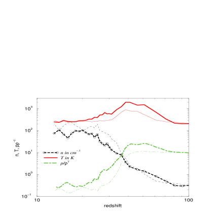
Figure 7: The evolution of the baryonic number density in ${\rm\ cm}^{-3}$ (dashed lines with circles indicating the data points), temperature in degrees Kelvin (solid lines), and the “entropy” function $p/\rho^{\gamma}$ which is invariant for adiabatic processes (dot–dashed lines) in arbitrary units for the densest zone in the simulation box of the $4\sigma 128$S (thin lines) and $4\sigma 512$S (thick lines) data. Here $p$, $\rho$, and $\gamma$ denote the gas pressure, density, and the adiabatic index, respectively.

This is what is illustrated in Figure 7 which shows the evolution of the “entropy” $p/\rho^{\gamma}$ (which is constant for adiabatic processes), the temperature, and the baryonic number density of the densest zone of the $4\sigma 128$S (thin lines) and $4\sigma 512$S (thick lines) data. Clearly for the $4\sigma 128$ simulation, the initial collapse at $z\lower 2.15277pt\hbox{$\;\buildrel>\over{\sim}\;$}45$ is adiabatic ($p/\rho^{\gamma}=const.$) and radiative cooling plays a role only at later redshifts. For the larger $4\sigma 512$ simulation box, the entropy increases in the redshift range $60\lower 2.15277pt\hbox{$\;\buildrel<\over{\sim}\;$}z\lower 2.15277pt\hbox{$\;\buildrel<\over{\sim}\;$}75$ due to merging and stays roughly constant thereafter until radiative cooling becomes important at $z\lower 2.15277pt\hbox{$\;\buildrel<\over{\sim}\;$}40$. H₂ cooling gives rise to a plateau in temperature until $z\lower 2.15277pt\hbox{$\;\buildrel<\over{\sim}\;$}38$ when it causes the temperature to decrease. Interestingly, we see that the central regions never reach the theoretical virial temperatures which are $\sim 2600{\rm\ K}$ for the $4\sigma 128$, and greater than $10^{4}{\rm\ K}$ for the $4\sigma 512$ run. Our simulations fail to resolve the core of these structures and hence the central density is not well defined once the gas in the most central structure has cooled. Therefore, the slow growth of the density for redshifts $10<z<30$ does not indicate that the collapse is halted.

The post–shock gas has been found to evolve isobarically in the case of radiative shocks (see, for example, Shapiro & Kang 1987 and Anninos & Norman 1996). Assuming the molecular hydrogen fraction increases according to equation (8) (see also Figure 8) and the isobaric evolution equation as discussed in section 2, one can determine the temperature evolution. For the central (densest) zone of our $4\sigma 128$S box, this isobaric evolution predicts that the gas would be able to cool to $\sim 30{\rm\ K}$ by redshift ten. The Lepp and Shull cooling function, which was used to derive the isobaric evolution, has been stated to be only valid to $100{\rm\ K}$. However, a new study by Tiné, Lepp, and Dalgarno (1997) confirms that the H₂ cooling timescale can be short even at lower temperatures. For example they find it to be of order $1{\,\rm Gyr}$ at a temperature of $50{\rm\ K}$ and a tenth of that at $70{\rm\ K}$ for typical H₂ fractions of $10^{-3}$ and $n_{H}\sim 100{\rm\ cm}^{-3}$. Hence if the gas evolves isobarically it will be able to cool to temperatures $\ll 100{\rm\ K}$. However, we see that the temperature and density, and hence the internal energy stay roughly constant at the final stages although the cooling time scales are short. This is due the extensive merging in the hierarchical scenario considered here, as well as our limited numerical resolution.

In section 2 we discussed the simple estimate of Abel (1995) and Tegmark et al. (1997) for the evolution of the H₂ fraction in a cloud derived solely in terms of its virial temperature and initial recombination timescale.

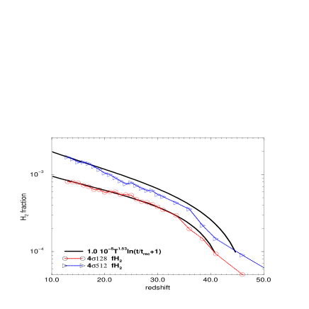
Figure 8: Molecular hydrogen fraction vs. redshift in the densest zone of the $4\sigma 128$S (open circles) and $4\sigma 512$S (triangles) simulations. The thick solid lines depict the approximating equation (8) initialized with the appropriate free electron densities, initial H₂ fraction, and temperature.

In Figure 8 we compare the predictions of equation (8) with the results from the $4\sigma 128$S (open circles) and the $4\sigma 512$S (triangles) runs. The fit is remarkably good, although the initial temperature (or redshift) is somewhat difficult to pick out in this case since the heating due to adiabatic compression is slow and the initial (virial) temperature is not as well defined for the larger mass scales. Analyzing the time derivative of equation (8) one finds for large times that $\dot{f_{H_{2}}}\propto T^{1.53}$ which, for the spherical collapse model, translates to $\dot{f_{H_{2}}}\propto M(1+z_{vir})^{1.53}$. This explains that the divergence of the two graphs in Figure 8 for low redshifts is due to the difference in the collapsing mass and collapse redshift.

Tegmark et al. (1997) have recently used a simple approach to derive the minimum mass scale that is able to collapse as a function of redshift. They model the density evolution in a cloud according to the predictions of the spherical collapse model, assuming the temperature increases adiabatically up to virialization and changes thereafter by radiative cooling. They simultaneously solve the rate equations for the time dependent chemistry to accurately predict H₂ formation and the subsequent cooling of the gas. We have reproduced their work with the same cooling function (Lepp & Shull 1983, hereafter referred to as LS) used in our cosmological hydrodynamics code to be able to directly compare their findings to our 3D numerical results.

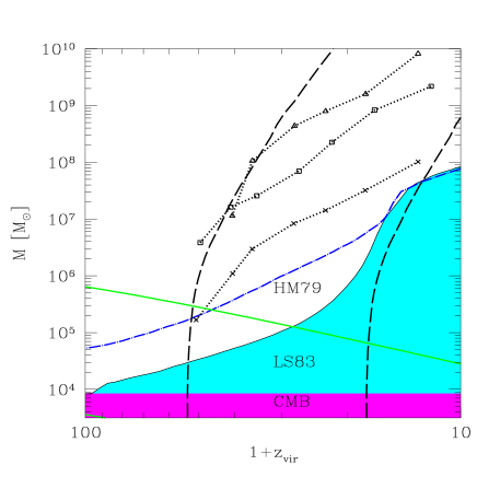
Figure 9: Total (baryonic and dark matter) collapsed mass vs. redshift. The horizontal dark shaded region depicts the mass scale for which the virial temperature equals the CMB temperature. The light shaded area (labeled LS83) represents the domain of parameters for which structures cannot collapse. This curve is computed assuming a spherical collapse model as in Tegmark et al. (1997), except we use the Lepp & Shull (1983) H₂ cooling function. Only above the light shaded area are structures believed to be able to collapse. The dotted lines show $M_{200}$ from our $3\sigma 128$S (crosses), $3\sigma 512$S (squares) and $3\sigma 1024$S (triangles) runs. The two dashed upward sloping lines depict the collapse redshift given by linear theory for the standard CDM spectrum scaled appropriately for $1\sigma$ and $3\sigma$ perturbations. The gray solid downward sloping line depicts the Jeans mass at $18\pi^{2}$ times the background density. The dot–dashed line is the original delimiting line computed by Tegmark et al. based on a modified form of the Hollenbach and McKee (1979) H₂ cooling function.

Figure 9 is analogous to Figure 6 of Tegmark et al. (1997) with our numerical results superimposed. The dotted lines are found by adding up all the mass in the $3\sigma$ simulations that is found within spherical shells on the sub grid in which the mean enclosed overdensity is 200. The collapse redshift agrees reasonably well with the predictions of linear theory, represented by the two dashed upward sloping lines. The use of different cooling functions has a very strong influence on the mass that can collapse, as evidenced by the difference in the two regions labeled HM79 (the Tegmark et al. result) and LS83 (our result). However, we note that although the quantitative results are very different, the shape for these two different $M_{c}(z)$ curves is rather similar at redshifts $30<z<100$. Their slope is consistent with $M_{c}\propto(1+z)^{-3/2}$, indicating a constant virial temperature since $T_{vir}\propto M^{2/3}(1+z)$. For the case in Tegmark et al. , the virial temperature in that redshift interval ($30<z<100$) is approximately $1000{\rm\ K}$. A constant virial temperature, in turn, implies a constant final H₂ fraction given by equation (8) which yields $f_{H_{2}}\sim 5\times 10^{-4}$ for $T_{vir}\sim 1000{\rm\ K}$ Comparing the cooling time scale to the dynamical time, they further argued that this H₂ fraction represents a universal value for which, if exceeded, the cloud will collapse at the free fall rate. This argument depends strongly on which cooling function is assumed. Using the Lepp and Shull (1983) H₂ cooling function, we find that the minimum virial temperature needed to produce enough molecules so that the gas can cool faster than its dynamical time is $\sim 200{\rm\ K}$ for redshifts $>30$. Which is five times smaller than the value derived from the modified Hollenbach and McKee (1979, hereafter HM79) cooling function used by Tegmark et al. . This smaller minimum virial temperature for the Lepp and Shull cooling function translates to a critical H₂ fraction of only $\sim 3\times 10^{-5}$. In our simulations, we find that the radius at which the baryonic overdensity exceeds the DM overdensity (see Figure 2) is coincident with the radius at which the fractional abundance of H₂ molecules exceeds $\sim 5\times 10^{-4}$. That we recover the critical H₂ fraction computed by Tegmark et al. , although we used the Lepp and Shull cooling function in our simulations, is hence coincidence.

5 Discussion and Summary

We have performed several three–dimensional numerical simulations of the first bound objects to form in a CDM model from high $\sigma$ fluctuations. In addition to evolving the dark and baryonic matter components, we have also solved a reaction network of kinematical equations for the chemistry important to the production of hydrogen molecules. The coupled system of chemical reactions and radiative cooling have been solved self–consistently, without recourse to any equilibrium or other simplifying assumptions. The accurate modeling of non–equilibrium cooling is crucial in determining the abundance of hydrogen molecules that form in the cores of collapsed objects. A range of baryonic mass scales $10^{3}$ – $10^{8}\ M_{\odot}$ (set by the range of box sizes) and formation epochs $15\lower 2.15277pt\hbox{$\;\buildrel<\over{\sim}\;$}z\lower 2.15277pt\hbox{$\;\buildrel<\over{\sim}\;$}70$ (set by both the mass scale and the normalization $\sigma$) have been investigated in this paper. The baryonic gas evolves to a complex network of sheets, filaments and knots with typical baryonic overdensities in the filaments of roughly an order of magnitude lower than at their intersections where $\rho/\overline{\rho}>200$. At all epochs and mass scales covered in our simulations, the heated gas in the filaments have characteristic temperatures that are typically a few times lower than in the spherical knots. Although we find the abundance of hydrogen molecules is enhanced throughout all the overdense or collapsed structures, the lower densities and temperatures of the filaments result in the lower fractional abundances of $n_{H2}/n_{H}\lower 2.15277pt\hbox{$\;\buildrel<\over{\sim}\;$}5\times 10^{-5}$ along the filamentary structures as compared to typical concentrations of $\lower 2.15277pt\hbox{$\;\buildrel>\over{\sim}\;$}5\times 10^{-4}$ in the spherical knots at the intersections of the filaments. This is understood from the analytical H₂ fraction evolution given in equation (8) which implies that hydrogen molecules form at slower rates in gas with lower initial temperatures and baryon densities. Since the H₂ cooling timescale in the low–density limit is proportional to $1/(n_{H}f_{H_{2}})$, it is clear why significant cooling is observed only at the cores of the highest density spheroidal structures, and not along the filaments. On the other hand, most of the volume in the simulations consists of expanding underdense voids. In these regions, the H₂ fraction equals the primordial background value of $\sim 3\times 10^{-6}$ since the densities and temperatures there are too low to further produce H₂ . Our findings are consistent with the results of Tegmark et al.  (1997) who used a simple spherical description of primordial collapsing clouds to estimate the minimum mass scale that can collapse for a given redshift. We have also justified the findings of Abel (1995) and Tegmark et al. (1997) that the molecular hydrogen fraction formed in structures at high redshifts arises initially solely through the residual free electrons left over from the incomplete recombination of the universe. Furthermore, our numerical results confirm the rule of thumb derived by Tegmark et al. that can be stated as: “Once the H₂ fraction is $\lower 2.15277pt\hbox{$\;\buildrel>\over{\sim}\;$}5\times 10^{-4}$ in a spherical primordial gas cloud and the gas temperature is well above $100{\rm\ K}$, the gas will be able to cool on timescales $\;\buildrel<\over{\sim}\;$ its dynamical one.”

We have not observed hydrogen molecules to trigger the initial collapse of perturbations at high redshifts. The adiabatically compressed core densities and temperatures in the initial phases of collapse are not high enough for the chemistry to generate a large abundance of hydrogen molecules. The gas therefore cannot cool before it collapses gravitationally and shock heats to temperatures greater than a few hundred degrees Kelvin. Our results thus confirm the conclusions of Haiman et al. (1996b) who found, using one–dimensional spherical models, that radiative cooling by H₂ affects the collapse of the baryonic gas only after it has fallen into the potential well of the dark matter halos and virialized. We note that Haiman et al. (1996b) overestimate the background H₂ fraction since they underestimated the photo–dissociation of H${}_{2}^{+}$ molecules at high redshifts through the CBR. This overestimation of the H₂ fraction in the background primordial gas, by two orders of magnitude, causes them to find that structures with virial temperatures as small as $120{\rm\ K}$ would be able to cool via H₂ . Consequently, their results on the history of H₂ formation in the virialized system cannot be correct. However, since they find that H₂ molecules cannot trigger the collapse of primordial structure despite the overestimated H₂ fraction, this result, which has been confirmed in this study, is robust. Although H₂ cooling does not trigger the collapse, it significantly influences the time evolution by keeping the temperatures in the central regions of the spherical knots to below the theoretical virial temperatures by at least a factor of a few, and by enhancing the baryon overdensities to $>10^{4}$. Furhermore we find H₂ cooling to cause a typical gas to DM density bias in the central regions similar to 4 times its background value.

Primordial stars can only form in the fraction of gas that is the able to cool. The fraction of cooled to total baryonic mass in the collapsed structures is only few percent. This is illustrated in Figure 10 which shows the ratio of cooled mass to $M_{200}$ as a function of redshift, where $M_{200}$ is the mass found within a spherical structure with a mean overdensity of 200. The amount of cooled gas is computed by adding up all the mass within the radius at which the temperature of the radially averaged profiles starts to decrease.

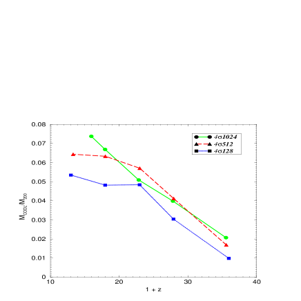
Figure 10: Evolution of the ratio of the cooled baryonic mass to the baryonic $M_{200}$ is shown for the 3 different (128, 512, & 1024 kpc box size) $4\sigma$ runs. The fraction of gas which cools approaches 5 to 8% towards the lower redshifts. The apparent slower growth of the structure in the $4\sigma 1024$S simulation is an artifact of grid resolution since the cooling flow is not resolved as well as in the smaller grids.

The bigger the box the more gas is able to finally cool, in agreement with the analytical picture where higher virial temperatures lead to larger molecular hydrogen abundances and hence shorter cooling timescales. The apparent slower growth of the structure in the $4\sigma 1024$ simulation is an artifact of grid resolution since the cooling flow is not resolved as well as in the smaller grids.

Padoan et al. (1997) put forward a theory for the origin of GCs in which the non-equilibrium formation of H₂ filters mass scales $\lower 2.15277pt\hbox{$\;\buildrel>\over{\sim}\;$}10^{8}\ M_{\odot}$ out of a CDM spectrum. In their model, these clouds convert about 0.3% of their total mass into a gravitationally bound stellar system and $\sim 2\%$ into halo stars. The remaining gas is enriched with metals and dispersed away from the GC by supernova explosions. Some of their assumed initial conditions are in agreement with what we find in our simulations. At redshift $z\sim 30$ a baryonic mass of about $10^{3}\ M_{\odot}$ has cooled to $T\sim 300{\rm\ K}$ (in the $4\sigma 128$ simulation). Although our numerical experiments fail to resolve the hydrodynamics within the cooled component, this sub–Jeans mass cold cloud may well host a complex supersonic random velocity field produced by isothermal shocks which are triggered by merger events with smaller surrounding structures. The gas stays isothermal since the H₂ cooling time scale is short, as can be seen in Figure 5. Therefore, this small cloud can likely form stars through the mechanism suggested by Padoan (1995). A perturbation of total mass $M$ contains $\Omega_{B}M$ baryons, of which a fraction $f$ can cool. Defining the star formation efficiency as $\epsilon$, the resulting mass in stars can be written as $M_{s}=\Omega_{B}f\epsilon M=5\times 10^{-5}M(\Omega_{B}/0.05)(f/0.05)(\epsilon/0.02)$. If one adopts the value of Padoan et al.  (1997) for the star formation efficiency ($\epsilon=0.02$) , the mass in stars formed in the smallest simulated structures of total mass $6.2\times 10^{5}\ M_{\odot}$ ($128{\rm\ kpc}$ box sizes) might be quite small $\sim 30\ M_{\odot}$. Hence, the first stellar systems formed in hierarchical structure formation scenarios, might be much smaller than thought previously.

Only two convincing detections of H₂ Lyman Werner Band absorption features in damped Ly$\alpha$ quasar absorption systems exist to date. The one system of Ge & Bechtold (1997) toward Q0013–004 has a very high reported H₂ fraction of $f_{H_{2}}=2N(H_{2})/[2N(H_{2})+N(HI)]=0.22\pm 0.05$ arguing for very efficient H₂ formation on dust grains. The second system found earlier by Levshakov and Varshalovich (1985) and confirmed by Foltz et al. (1988) toward PKS 0528–250 shows an H₂ fraction of $\sim 2\times 10^{-3}$ which is a typical value for primordial structure formation as we have seen above. Since the H₂ column density in this system is $\sim 10^{18}{\rm\ cm}^{-2}$ it will be self–shielded from intergalactic radiation allowing the H₂ formed during the initial collapse of that system to survive the UV flux from the quasar. Unfortunately this system shows an absorption redshift greater than the emission redshift of the background quasar and is therefore likely to be physically influenced by the quasar. Furthermore, its high Doppler parameter of $b=100\,{\rm{km\,s^{-1}}}$ found for the HI component suggests that the absorption originates in a systems larger then the objects discussed here. It is nevertheless interesting that the H₂ fraction, HI column density, and the reported excitation temperature of $T_{exc}\sim 100{\rm\ K}$ (Foltz et al. 1988) can be found for halos with virial velocities exceeding $10\,{\rm{km\,s^{-1}}}$ that collapse at high redshifts, $z\lower 2.15277pt\hbox{$\;\buildrel>\over{\sim}\;$}10$ (see Abel & Mo 1997). I.e. systems as the ones simulated in this investigation.

None of the investigations that have implemented a self–consistent treatment of the H₂ chemistry and cooling with the hydrodynamics of collapsing structures (ie. Anninos & Norman, 1996; Haiman et al. , 1996; this work; Abel et al. 1997) have formed baryonic overdensities greater than $10^{5}$. For some of these studies, this can perhaps be attributed to the lack of numerical resolution. However, we would like to stress that currently no self–consistent model of primordial star formation exists. As a next step towards an understanding of the origin of the first star in the universe we are currently implementing our chemistry/cooling model into the Berger and Oliger (1984) adapted mesh refinement (AMR) scheme to provide dramatic improvements in the dynamic range of both mass and length scales. This approach will allow us to resolve the core of the cooling structures and address questions that remain unanswered by this and previous studies.

Figure 11: Contour surfaces showing an evolution sequence for the dark matter and baryonic gas overdensities at redshifts $z=$ 35, 22, 17 and 12. Five levels (0.5, 1, 1.5, 2, 2.5) are displayed for $\log\rho/\overline{\rho}$, where $\overline{\rho}$ is the background density. Each individual plot represents a single slice at a fixed $z$ coordinate, intersecting the densest cell on the top grid for the 3$\sigma$ run with box size $L=512~{}kpc$.

Figure 12: As in the previous figure, but for the higher resolution sub grid.

Figure 13: Contour surfaces showing an evolution sequence for the gas temperature and H₂ fraction $n_{H2}/n_{H}$ at redshifts $z=$ 35, 22, 17 and 12. Five levels are displayed for both the temperature ($\log T(eV)=$ -2.2, -2, -1.5, -1, -0.5) and the H₂ fraction ($\log n_{H2}/n_{H}=$ -5.05, -5, -4.5, -4, -3.5).

References

- (1)
- (2) bel, T., 1995, thesis, Univ. Regensburg.
- (3) bel, T., Anninos, P., Zhang, Y., & Norman, M.L. 1997a, NewA, accepted (astro-PH 9608040).
- (4) bel, T. & Mo, H.J. 1997, in preparation.
- (5) bel, T., Stebbins, A., Anninos, P., & Norman, M.L. 1997b, in preparation.
- (6) nninos, P. & Norman, M.L. 1996, ApJ, 460, 556.
- (7) nninos, P., Norman, M.L., & Clarke, D.A. 1994, ApJ, 436, 11.
- (8) nninos, P., Zhang, Y., Abel, T., & Norman, M.L. 1997, NewA accepted (astro-PH 9608041).
- (9) erger, M.J. & Oliger, J. 1984, J. Comp. Phys., 53, 484.
- (10) ertschinger, E. 1994, Private Communication.
- (11) odenheimer, P.H. 1986, Final Technical Report, California Univ., Santa Cruz.
- (12) opi, C.J., Schramm, D.N., & Turner, M.S. 1995, Science, 267, 192.
- (13) ouchman, H.M.P. & Rees, M.J. MNRAS, 1986, 221, 53.
- (14) erland, G.J., Peterson, B.M., Horne, K., Welsh, W.F., & Nahar, S.N. 1992, ApJ, 387, 95-108.
- (15) oltz, C.B., Chaffee, Jr., F.H., & Black, J.H. 1988, ApJ, 324, 267.
- (16) e, J., & Bechtold, J. 1997, ApJ, 477, L73.
- (17) nedin, N.Y. & Ostriker, J.P. 1997, submitted to ApJ.
- (18) unn, J.E., & Gott, J.R. 1972, ApJ, 432, 1.
- (19) aiman, Z., Rees, M.J., & Loeb, A. 1997, ApJ, 476, 458.
- (20) aiman, Z., Rees, M.J., & Loeb, A. 1996a, ApJ, 467, 522.
- (21) aiman, Z., Thoul, A.A., & Loeb, A. 1996b, ApJ, 464, 523.
- (22) ollenbach, D. & McKee, C.F. 1979, ApJS, 342, 555.
- (23) utchins, J.B. 1976, ApJ, 205, 103.
- (24) epp, S. & Shull, J.M. 1983, ApJ, 270, 578.
- (25) evshakov, S.A., & Varshalovich, D.A. 1985, MNRAS, 212, 517.
- (26) ac Low, M.-M. & Shull, J.M. 1986, ApJ, 302, 585.
- (27) avarro, J.F., Frenk, C.S., & White, S.D.M. 1996, ApJ, 462, 563.
- (28) adoan, P. 1995, MNRAS, 277, 377.
- (29) adoan, P., Jimenez, R., & Jones B.J.T. 1997, MNRAS, 285, 711.
- (30) alla, F., Salpeter, E.E., & Stahler, S.W. 1983, ApJ, 271, 632.
- (31) eebles, P.J.E. 1968, ApJ, 153, 1.
- (32) eebles, P.J.E. 1993, Principles of Physical Cosmology, (Princeton University Press, NJ).
- (33) ress, W.H. & Schechter, P. 1974, ApJ, 187, 425.
- (34) aslaw, W.C. & Zipoy, D. 1967, Nature, 216, 976.
- (35) hapiro, P.R. & Kang, H. 1987, ApJ, 318, 32.
- (36) unyaev, R.A. & Zel’dovich, Ya.B. 1972, å, 20, 189.
- (37) egmark, M., Silk, J., Rees, M.J., Blanchard, A., Abel, T., Palla, F. 1997, ApJ, 474, 1.
- (38) iné, S., Lepp, S., & Dalgarno, A. 1997, in preperation.
- (39) hang, Y., Anninos, P., & Norman, M.L. 1995, ApJ, 453, L57.
- (40) hang, Y., Norman, M.L., Anninos, P., & Abel, T. 1996, to appear in the proceedings of the 7th Annual Astrophysics Conference in Maryland, Star formation, near and far, eds. Stephen S. Holt and Lee G. Mundy.