Cosmology with Sunyaev-Zeldovich observations from space

Abstract

In order to assess the potential of future microwave anisotropy space experiments for detecting clusters by their Sunyaev-Zeldovich (SZ) thermal effect, we have simulated maps of the large scale distribution of their Compton parameter $y$ and of the temperature anisotropy $\Delta T/T$ induced by their proper motion. Our model is based on a predicted distribution of clusters per unit redshift and flux density using a Press-Schecter approach (De Luca et al. 1995).

These maps were used to create simulated microwave sky by adding them to the microwave contributions of the emissions of our Galaxy (free-free, dust and synchrotron) and the primary Cosmic Microwave Background (CMB) anisotropies (corresponding to a COBE-normalized standard Cold Dark Model scenario). In order to simulate measurements representative of what current technology should achieve, “observations” were performed according to the instrumental characteristics (number of spectral bands, angular resolutions and detector sensitivity) of the COBRAS/SAMBA space mission. These observations were separated into physical components by an extension of the Wiener filtering theory (Bouchet et al. 1996). We then analyzed the resulting $y$ and $\Delta T/T$ maps which now include both the primary anisotropies and those superimposed due to cluster motions. A cluster list was obtained from the recovered $y$ maps, and their profiles compared with the input ones. Even for low $y$-values, the input and output profiles show good agreement, most notably in the outer parts of the profile where values as low as $y\simeq 3.\,10^{-7}$ are properly mapped. We also construct and optimize a spatial filter which is used to derive the accuracy on the measurement of the radial peculiar velocity of a detected cluster. We derive the accuracy of the mapping of the very large scale cosmic velocity field obtained from such measurements.

1 Introduction

Future space experiments should allow to built a large statistically homogeneous sample of clusters of galaxies detected by the spectral signature of CMB photons scaterring off the free electrons of the hot intra-cluster gas. This would be of great cosmological interest, allowing to constrain the cosmological scenarios of large scale structure formation and evolution, as well as the gas history (Colafrancesco & Vittorio1994, Barbosa et al. 1996).

The measurement of the peculiar velocity of clusters of galaxies could be an important tool to study the large scale velocity field of the universe. This in turn provides a unique opportunity for probing the underlying mass distribution. Thus one can probe fairly directly the primordial spectrum and further constrain the various cosmological models. The direct determination of the peculiar velocity (by independent redshift and distance determination) is observationally difficult and time-consuming. Still, several groups have succeeded in measuring the bulk, volume-averaged, peculiar velocity field, in our neighborhood, on scales $r=10\,h^{-1}$ to $60\,h^{-1}$ Mpc (Aaronson et al. 1986, Collins et al. 1986, Dressler et al. 1987, Strauss & Willick 1995 (for a recent review)).

Another method is nevertheless possible. It relies on combining the informations from the Sunyaev-Zeldovich (SZ) effects (thermal and kinetic) which create secondary temperature fluctuations (Zeldovich & Sunyaev 1969, Sunyaev & Zeldovich 1972, 1980). The combination of the measurements of the two effects give a fairly direct determination of the peculiar radial velocity of clusters of galaxies (Sect. 2.2, Eq. 3), although a good estimate of the peculiar velocity requires a precise measurement of both SZ effects and of the gas temperature. A crucial advantage of such a combination is that the SZ effects do not decrease in brightness with distance. Therefore measurements of both effects for a large number of clusters could give precise estimates of the large scale velocity field distribution.

The temperature fluctuations generated by the kinetic SZ effect have the same spectral signature than the primordial anisotropies of the CMB. For cluster velocity determinations, the primordial temperature fluctuations of the CMB act as a contaminating source of the SZ kinetic effect. In addition, one must also take into account all other sources of contamination that might spoil the measurement, from resolved sources (other clusters, galaxies …), unresolved ones (galactic synchrotron, free-free emission …) or instrumental noise.

Some measurements of the SZ thermal effect, on known clusters, have already been made in the wavelength range where the SZ effect creates a decrement in the CMB intensity ($\lambda>1.3$ mm) (see Rephaeli 1995 and references therein).

In the context of the feasibility study of future space projects such as the COBRAS/SAMBA mission, of the European Space Agency, dedicated to the CMB observations together with other cosmological targets (SZ detection in clusters, primordial galaxies, …), a complete simulation of the astrophysical processes, the expected instrumental characteristics of the satellite and of the separation of these processes was performed (Bouchet et al. 1996). This simulation was used as a tool to constrain and quantify the capabilities of the satellite. In this paper, we focus on the capabilities of such a mission for the detection of the SZ thermal effect of clusters of galaxies, the imaging of the clusters and finally the measurement of their peculiar velocities.

Section 2 introduces briefly the formalism of the thermal and kinetic SZ effects, while we present in section 3 the method we used to generate SZ effect maps. Section 4 assesses the capabilities of a space experiment like COBRAS/SAMBA to detect clusters, and we evaluate, in section 5, the accuracy of the peculiar velocity determination of individual clusters. We finally derive the expected accuracy on the rms dispersion of the large scale velocity field in section 6. Section 7 summarizes the main results and conclusions of the paper.

2 Sunyaev-Zeldovich thermal and kinetic effects

2.1 Thermal Sunyaev-Zeldovich effect

The thermal SZ effect is the inverse Compton scattering of CMB photons by free electrons in the hot intra-cluster medium. Since the number of photons is conserved, their spectrum is just shifted on average to higher frequencies.
This effect is characterized by the comptonization parameter $y$, which depends only on the cluster’s electronic temperature and density ($T_{e}$, $n_{e}$):

$$y=\frac{k\sigma_{T}}{m_{e}c^{2}}\int T_{e}(l)n_{e}(l)dl$$

where $k$ is the Boltzmann constant, $\sigma_{T}$ the Thomson cross section, $m_{e}c^{2}$ the electron rest mass energy and $l$ is the distance along the line of sight. When the intra-cluster gas is isothermal ($T_{e}(l)=T_{e}=const$), $y$ is expressed as a function of the optical depth $\tau$ ($\tau=\sigma_{T}\int n_{e}(l)\,dl$):

$$y=\tau~{}\frac{kT_{e}}{m_{e}c^{2}}.$$ (1)

The relative monochromatic intensity variation of the CMB due to the SZ thermal effect is given by

$$\frac{\Delta I_{\nu}}{I_{\nu}}=y\cdot f(x)$$

where $x$ is the adimentionnal frequency $x=h\nu/kT_{CMB}$ ($h$ denotes the Planck constant, $T_{CMB}$ the CMB temperature, and $\nu$ the frequency), $I_{\nu}$ is the intensity of the CMB (black body emission) and $f(x)$ is the spectral form factor given by:

$$f(x)=\frac{xe^{x}}{(e^{x}-1)}\left[x\left(\frac{e^{x}+1}{e^{x}-1}\right)-4\right].$$

2.2 Kinetic Sunyaev-Zeldovich effect

If a cluster has a radial peculiar velocity $v_{r}$, another relative intensity variation of the CMB due to the Doppler first-order effect is added. It is given by:

$$\frac{\Delta I_{\nu}}{I_{\nu}}=-\frac{v_{r}}{c}\tau\cdot a(x)=\left(\frac{\Delta T}{T}\right)_{SZ}\cdot a(x),$$ (2)

where $a(x)$ is the spectral form factor for the kinetic effect, given by:

$$a(x)=x\frac{e^{x}}{e^{x}-1},$$

and $\tau$ is the optical depth. The effect is positive for clusters moving towards the observer (i.e. with negative velocities).

The intensity fluctuation induced by the SZ kinetic effect has the same spectral shape as the primordial ones (equivalent to a temperature fluctuation).

The temperature variation due to the kinetic SZ effect can be written as a function of the $y$ parameter (defined in Eq. 1). The combination of the two SZ effects gives the expression of the radial velocity of the cluster:

$$v_{r}=-c\,\frac{kT_{e}}{m_{e}c^{2}}\frac{(\Delta T/T)_{SZ}}{y}.$$ (3)

At high frequencies, the expressions given above are not accurate enough and relativistic calculations of the thermal effect are needed in most cases (Rephaeli 1995 and references therein). A relativistic treatment introduces differences in the relative intensity variation and a shift of the crossover frequency. The corrections depend on both the temperature of the intracluster medium and the frequency. In this paper, we have restricted our study to the nonrelativistic treatment as a “text book” case in order to adress the capabilities of a space mission in measuring the SZ effect on clusters of galaxies. The corrections for the relativistic case will have to be taken into account when dealing with real data.

3 Simulations

3.1 Cluster model

We model the $y$ profile of a single resolved cluster according to a King model (King 1966). The main physical characteristics of the cluster are $n_{e}(R)$ and $T_{e}(R)$, respectively the electronic density and temperature distributions given as functions of the distance $R$ to the center of the cluster. Hereafter, we use a hydrostatic isothermal model with a spherical geometry (Cavaliere & Fusco Femiano 1978, Birkinshaw, Hugues & Arnaud 1991). For the density distribution, this gives:

$$n_{e}(R)=n_{e0}\left[1+\left(\frac{R}{R_{c}}\right)^{2}\right]^{-\frac{3\beta}{2}},$$

where $n_{e0}$ is the central electronic density, $R_{c}$ is the core radius and $\beta$ is a parameter of the model which represents the ratio of the kinetic energy per unit mass in the galaxies to the one in the gas. We take $\beta=2/3$, as indicated by both numerical simulations (Evrard 1990) and X-ray surface brightness profiles (Jones & Forman 1984, Edge & Stewart 1991). The hypothesis of isothermality is rather well confirmed by the X-rays observations of the ASCA satellite (Mushotzky 1994).

In this specific model for the gas distribution, the integrated $y$ profile of the cluster is given by:

$$y\propto\left[1+\left(\frac{\theta}{\theta_{c}}\right)^{2}\right]^{-1/2},$$

$\theta$ and $\theta_{c}$ being respectively the angular distance to the center of the cluster and core radius. The Full Width at Half Maximum (FWHM) of the profile and the core radius of the cluster are related by $FWHM=3.5\times\theta_{c}$.

For the time evolution of the temperature $T_{e}$ and core radius $R_{c}$, we use the model of Bartlett and Silk (1994) in which the main parameters of the cluster evolve as suggested by the self-similarity arguments (Kaiser 1986), with a parameter standing for the negative evolution of the number of clusters indicated by the X-ray observations. The normalization of the temperature and core radius is made using the A665 ASCA data (Yamashita 1994).

3.2 The maps

We simulate $500\times 500$ pixels ($12.5^{\circ}\times 12.5^{\circ}$) maps of the clusters, in terms of their $y$ parameters for the thermal SZ effect and $\Delta T/T$ maps of the same size for the kinetic SZ effect. The distribution of clusters per unit of redshift, solid angle and flux density interval was computed (De Luca et al. 1995) using a Press-Schechter mass function (Press & Schechter 1974) normalized to X-ray and optical data (Bahcall & Cen 1993). The total number of sources in each map is drawn using a Poisson distribution, the position of each cluster being also assigned at random, i.e. the effect of spatial correlations are not taken into account.

The counts in De Luca et al. (1995) are obtained using a formalism similar to the one adopted in Bartlett & Silk (1994) taking into account the negative evolution in time suggested by X-ray observations.

A discrimination between resolved and unresolved clusters is made according to their spatial extent. We give the gas distribution within clusters a finite extent with a maximum radius $R_{max}$. In fact, the hydrodynamic isothermal model is in good agreement with X-ray observations over 5 core radii (Markevitch et al. 1992), other observations (Henriksen & Mushotzky 1985) show that in some cases the gas in clusters is still seen up to 10 core radii. This seems to be also the case in the ASCA data (Mushotzky 1994). These sizes are the ones estimated from the X-ray observations. Since the X-ray emisssion is proportional to $n_{e}^{2}$, the observations are strongly biaised towards the center of the clusters and tend to minimize the extent of the clusters. Recent simulations of cluster formation (Evrard et al. 1996) show that the virialization limit for the clusters takes place at 2 to 3 Mpc from the center. For typical values of the core radius (0.1 to 0.2 Mpc) the dynamical extent of the clusters is thus of the order of 10 to a few tens of core radii. Because the SZ effect is proportional to the $n_{e}$, it is therefore very sensitive to the outer parts of the density profile where most of the mass rests. In order to investigate the case where the clusters extend beyond the estimations from X-rays, we assume, for the simulated maps, that the maximum extent of a cluster is $20\theta_{c}$ with a profile going down to zero for $\theta>10\theta_{c}$. In the maps, the unresolved sources are thus the ones for which $20\theta_{c}<1.5^{\prime}$, where $1.5^{\prime}$ is the simulation pixel size. In that case, we assign to the corresponding pixel an integrated $y$ parameter, noted Y (see Eq. 4). When the sources are spatially resolved ($20\theta_{c}>1.5^{\prime}$), we compute their $y$ profile using the above $\beta$-model for the gas (Sect 3.1 and appendix A).

To generate the $\Delta T/T$ maps arising from the SZ kinetic effect, the radial peculiar velocity $v_{r}$ of each cluster is drawn randomly from an assumed Gaussian velocity distribution with standard deviation today $\sigma_{0}=400\,km/s$ (Faber et al. 1993). The time evolution of the standard deviation is followed according to linear perturbation theory. We also assume no correlations in the velocity distribution. Using the same procedure than above concerning the source extents, we compute $\Delta T/T$ profiles for the resolved clusters (Appendix A).
We found that this simple model based on De Luca et al. (1995) modeling for the SZ source counts turns out to be in rather good agreement with Bond & Myers’ (1996) more sophisticated simulations, based on the “peak patch” algorithm, at least for statistical quantities such as the $rms$ values of both the $y$ parameter and $\Delta T/T$. This justifies the approximations made concerning correlations.

4 Detection and mapping of distant clusters

It is now possible, due to recent technological improvements, to design a new generation of satellites dedicated to CMB observations at small angular scales (few arcminutes to few degrees) with very high sensitivities, allowing the detection of temperature fluctuations at a level of $\Delta T/T\simeq 10^{-6}$. Measuring primordial temperature fluctuations at this level of accuracy requires the ability to detect secondary fluctuations such as the ones associated with the SZ effect. Therefore one of the byproducts of such a survey of the CMB will certainly be a new catalogue of clusters of galaxies.
The physics of cluster formation and the history of gas virialization are still almost unknown. The SZ effect measurement provides a new method of observing clusters which is potentially more powerful than X-ray observations for the search of clusters at high redshifts.

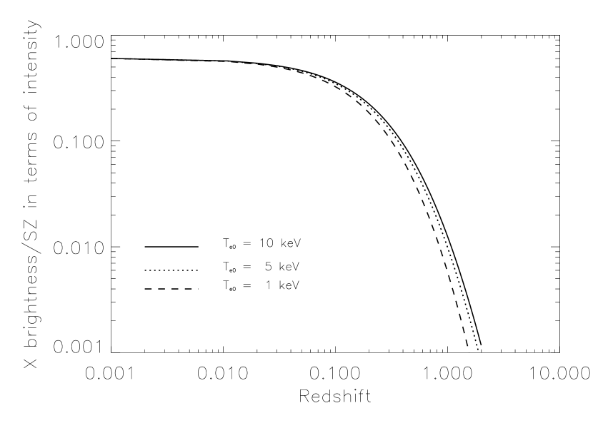
Figure 1: Ratio of the X brightness to the intensity of the SZ thermal effect as a function of the redshift, for three temperatures of the cluster.

Figure 1 gives the ratio of the X-ray brightness of a galaxy cluster to the intensity of its SZ thermal effect, as a function of the redshift. It shows that at $z=1$ the X-ray brightness drops by a factor greater than 30 compared to the SZ intensity, indicating that SZ observations should be very powerful to detect high $z$ clusters.

In the context of CMB observations at small angular scales with high sensitivities, the problem of the detectability of clusters among the other astrophysical components is essential to evaluate how many clusters could be found in a sky survey, especially at large distances. Fortunately, the SZ thermal effect, which has a specific spectral signature (positive and negative intensity peaks at respectively 0.85 and 2 mm with a zero value at 1.38 mm), is rather easy to identify in the framework of a multi-frequency experiment covering the range 30 to 800 GHz, with high sensitivities and good angular resolution such as COBRAS/SAMBA. Using the separation of processes (primordial CMB, clusters, free-free, …) which is based on the projection of the “observed” signal in different wavebands (Bouchet et al. 1996), the sky simulation provides us with a recovered $y$ map for the SZ thermal effect together with a $\Delta T/T$ map. These recovered maps are used to characterize the number of clusters that could be detected and furthermore they show the ability of the survey to image the clusters.

In order to find the detected clusters in the recovered $y$ maps, we use the following algorithm. Above a threshold of $y=2.\,10^{-6}$, each maximum is associated with the central peak of the $y$ profile of a resolved cluster. Assuming spherical symmetry, we compute the radial profile of the comptonization parameter $y$, by averaging within rings of equal width. We also compute the integrated $y$ parameter, Y, over the profile for each recovered cluster. Then, we compare these reconstructed profiles with the input ones. We thus produce a catalogue of detected clusters giving the position of the $y$ maxima in the map, together with the “measured” central value $y_{0}$, and the integrated parameter Y. The method, which consists of integrating the signal over rings getting larger and larger, tends to overestimate the signal if one does not take out a base line which is the average $y$ value given by undetectable weak clusters. For rings of constant $\delta R/R$, both noise and signal decrease as $1/R$ where $R$ is the distance to the center of the cluster; thus the signal (integrated over rings) to noise ratio is constant as long as the density follows a $\beta$-profile.

Figure 2: Input (solid line) and recovered (dashed) profiles for a cluster with high $y$ as a function of the distance to center in arcminutes. The integrated $y$ parameter is recovered with better than 2%

Figure 3: Input (solid line) and recovered (dashed) profiles for a cluster 100 times weaker than typical observed clusters. Here, the intagrated $y$ parameter is recovered with an accuracy of 12%.

Figures 2 and 3 show both input and recovered profiles for respectively a strong cluster (in terms of the $y$ parameter) and a weak one, very close to the sensitivity limit of the COBRAS/SAMBA instruments. In both figures we note that the central part of the cluster suffers from the beam dilution, this region is therefore not recovered in a satisfactory way by the SZ observations. On the other hand, the wings of the cluster are well recovered, they are observable down to $y\approx 3.\,10^{-7}$ over about one degree as indicated in Fig. 2. The comparison between the input and recovered profiles shows a good agreement. In fact, the sensitivity is such that clusters, and specifically the wings of the profile, can be observed through the SZ thermal effect as far as the gas extends; the main limit to such a measurement is likely to be the confusion limit, due to the overlap of weak clusters in the background. The ability to detect the wings of the profiles indicates that the SZ effect is a powerful tool to constrain gas accretion models in potential wells of clusters and measure the virialization radius which gives the spatial extent of a cluster. Furthermore, more information in the statistical properties of the distribution of the comptonization parameter $y$ can be extracted and used to constrain evolution models even when confusion sets in.

The X-ray emission and the SZ effect are dominated by different parts of the cluster; X-rays are mainly associated with the core of the cluster because the intensity of bremstrahlung emission is proportional to $n_{e}^{2}$, whereas the SZ effect which is proportional to the electron column density is dominated by contributions coming from the lower density regions where the path length is longer. Therefore, the information brought by both X-rays and the SZ effect are quite different and rather complementary.

A comparison between the capabilities of X-ray and SZ measurements for clusters can be done by using the characteristics of the EPIC camera planned for the X-ray observatory mission XMM and the COBRAS/SAMBA characteristics. Due to their good resolution and because they are biaised by the $n_{e}^{2}$ dependence, X-ray observations are well adapted to map the core of the clusters. The EPIC-XMM instruments can map the cluster up to about $7\theta_{c}$ at a sensitivity of $5\sigma$ reached in 20 hours of integration. This is illustrated in figure 4 for an A496-like cluster ($T_{e0}=4$ keV at $z=0.2$). The EPIC instrument will map the clusters (especially the central part) and will give the temperature distribution, electronic density… The SZ observations suffer from a significant beam dilution of the core, because of the lack of resolution compared with the X-rays measurements, but they resolve the wings of the cluster profile up to the virialization limit (cf. Fig. 2). Figure 4 shows that the A496-like cluster is mapped up to about $17\theta_{c}$ with SZ observation. Therefore, a combination of X-ray measurements together with SZ observations will strongly constrain cluster models.

Figure 4: Comparison between X-ray brightness (solid line) and the $y$ parameter (dotted line) for a A496-like cluster ($T_{e0}=4$ keV at $z=0.2$) with XMM-EPIC and COBRAS/SAMBA resolutions, respectively for the X-rays and $y$ observations. Left axis: X-ray brightness in EPIC counts/s/arcmin²; right axis: $y$ paramter, versus angular size in arcmin. The solid horizontal line stands for the X-ray background, the sensitivity limit of the XMM instrument for an integration time of 20 hours is indicated by the dashed horizontal line whereas the dotted line is for the COBRAS/SAMBA sensitivity limit.

A high sensitivity SZ sky survey like the one that can be carried out by a mission like COBRAS/SAMBA will give the best catalogue of distant clusters and will be used to define follow-up observations with X-ray observations which require a long integration time to study a distant cluster.

One can characterize the clusters in terms of their measurable parameters: angular core radius $\theta_{c}$, central value of the comptonization parameter $y_{0}$ or the integrated parameter Y, which combines the two previous quantities. Assuming a King profile, this parameter is directly related to the mass of the gas, the redshift $z$ and the temperature of the clusters, by the following expression (for a flat universe):

$$\int\frac{y~{}d\Omega}{10^{-4}~{}\mbox{arcmin}^{2}}=0.43h^{2}\left(\frac{M_{G}}{10^{14}M_{\odot}}\right)\left(\frac{kT_{e}}{10~{}keV}\right)$$

$$\frac{(1+z)^{3}}{(\sqrt{1+z}-1)^{2}}.$$ (4)

In terms of observable parameters, Y is given by ${\mbox{Y}}=64\,y_{0}(\theta_{c}/\mbox{arcmin})^{2}$. We expect that the extraction of the clusters will depend mainly on the value of Y, because the sensitivity of the SZ profile does not decrease with radius as long as the gas density decreases as $R^{-2}$.Thus, the sensitivity required to detect a cluster is controled by the integrated emission and not by the peak brightness.

We use the extraction method described above, applied to the simulated input and recovered maps and derive the completeness of the obtained catalogue of resolved clusters as a function of their Y.

Figure 5: Fraction of the recovered clusters from a recovered map after component separation, for three sensitivities as a function of the integrated Y comptonization parameter. The nominal mission of COBRAS/SAMBA is 14 months of observations.

A systematic extraction of the clusters is done for three noise configurations (the nominal observing time for COBRAS/SAMBA mission is about one year). Both 48 and 12 months of observations enable the detection of at least 95% of the clusters with Y $>9.\,10^{-4}\,\mbox{arcmin}^{2}$. For the 12 months configuration, 70% of the clusters with Y $>5.\,10^{-4}\,\mbox{arcmin}^{2}$ and $y_{0}>3.\,10^{-6}$ are recovered. For such clusters, the integrated $y$ parameter is recovered, on average, with an accuracy of about 30% (clusters shown in figures 2 and 3, the accuracies are respectively 1.4% and 12%). Decreasing the noise level leads obviously to a deeper survey as indicated in the plot (Fig. 5). If we increase the noise level to a noise corresponding to a 6 months mission, even some of the strongest clusters are not detected. In fact, we recover only 85% of clusters for which ${\mbox{Y}}>10^{-3}\,\mbox{arcmin}^{2}$, and the extraction gets worse for clusters with ${\mbox{Y}}=5.\,10^{-4}\,\mbox{arcmin}^{2}$.

By using the De Luca et al. (1995) source counts model, we expect that a mission like COBRAS/SAMBA could detect about $7.\,10^{3}$ resolved clusters with ${\mbox{Y}}>9.\,10^{-4}\,\mbox{arcmin}^{2}$ and a completeness better than 95%, and about $10^{4}$ clusters with ${\mbox{Y}}>5.\,10^{-4}\,\mbox{arcmin}^{2}$ and completeness better than 68%. These numbers are very model dependent and could increase by a factor 3 for cosmological models with low $\Omega_{0}$ due to the existence of distant clusters ($z>0.5$) and their contribution to the counts as in the model of Barbosa et al. 1996.

5 Peculiar velocity measurement

Given the radial peculiar velocities at known positions and under the assumption of a potential velocity flow around our galaxy, one can extract the velocity field and derive the bulk velocity $V_{R}$ which is the average of the local velocity field smoothed over a window function of scale $Rh^{-1}$ Mpc. One can get the peculiar radial velocities using the redshift surveys and some relationships, giving the distances to the objects, such as the Faber-Jackson (1976) or Tully-Fisher (1977) relations. Several authors have measured the bulk velocities averaged over different volumes (a good approximation at very large scales), Dressler et al. (1987) found $V_{60}=599\pm 104$ km/s, Courteau et al. (1993) measured $V_{40}=335\pm 38$ km/s and $V_{60}=360\pm 40$ km/s, Willick et al. (1996) computed the bulk velocity using POTENT they found $V_{60}=20-300$ km/s. The main difficulty from which this method suffers is that it requires very reliable distance indicators. Therefore, the relative error in determining the peculiar velocity increases with distance.

The determination of the peculiar velocity from SZ measurement is promising, since its accuracy is distance independent. If indeed one can detect the kinetic SZ effect for a number of clusters as large as $10^{4}$ (as possible with the COBRAS/SAMBA mission), this will provide unique statistical information on the velocities.

5.1 Calculation method and geometrical filter

The radial peculiar velocity of the cluster is given by combining the measurements of both kinetic and thermal SZ effects (Sect. 2.2, Eq. 3). The components separation takes advantage of the spectral signatures of the different astrophysical contributions (free-free, synchroton, clusters of galaxies, …), which are taken into account in the sky simulation (Bouchet et al. 1995), and of the characteristics of the instrument to give recovered maps of the astrophysical processes. In particular, the $\Delta T/T$ map, obtained after the components separation, includes both primordial CMB fluctuations and $(\Delta T/T)_{SZ}$ because they have the same spectral signature. The $(\Delta T/T)_{SZ}$ is thus contaminated by the primordial temperature fluctuations of the CMB, this contamination beeing responsible for an error in the determination of the peculiar radial velocity of a cluster when one uses a method based on the combination of measurements of both SZ effects. The aim is to have the smallest error on the velocity, this requires a good measurement of $(\Delta T/T)_{SZ}$.

The induced temperature fluctuations due to the SZ kinetic effect have angular sizes smaller than one degree, whereas the CMB spectrum exhibits a “Doppler” peak at about one degree. Within this framework, a good measurement of the SZ kinetic effect (and thus the peculiar velocity) must be a compromize between on the one hand maximizing the signal by integrating over a large beam, and on the other hand minimizing the spurious contribution from the CMB.

The peculiar radial velocity of a cluster is given by

$$v_{r}=\frac{ck}{m_{e}c^{2}}\times T_{e}\frac{\Delta T/T}{y}.$$

The relative error in the velocity is thus expressed as follows:

$$\frac{\delta v_{r}}{v_{r}}=\frac{\delta A}{A}+\frac{\delta T_{e}}{T_{e}},$$ (5)

where $A=\frac{\Delta T/T}{y}$. The error due to the CMB contamination appears in the measurement of the temperature fluctuation $\Delta T/T$ and it is measured using a spatial filter that optimizes the signal to “noise” ratio (the main “noise” being the primary CMB). The $\Delta T_{e}/T_{e}$ term is the error due to the uncertainty on the intracluster gas temperature determination. It should be derived from X-ray data. Hereafter, we do not include it in the evaluation of the $\frac{\delta v_{r}}{v_{r}}$.

To minimize the contamination of the CMB, we construct a spatial filter over which we calculate a variation of both $\Delta T/T$ and $y$ on a single cluster. The spatial filter used hereafter computes the difference between the mean values of $\Delta T/T$ and $y$ in the central part of the cluster and their mean values taken in a ring around the peak. This filter has three free parameters, one is the radius of the central disc and the two others the inner and outer ring radii.

If the noise due to the spurious signals is dominated by a single component of a known power spectrum, the spatial filter can be optimized (Haenhelt & Tegmark 1996). In practice, several sources contribute to the noise including some non gaussian ones like the confusion of weaker clusters. Furthermore, we adress the problem of the optimization of the filter using only the informations included in the data. The shape and size of the optimum filter depend on the extent of the cluster and its density profile. We thus empirically optimize the simple filter in the case of one cluster model (King profile) and one primordial CMB spectrum (standard CDM with $\Omega_{b}=0.05,h=0.5$ and $\Omega_{0}=1$) to evaluate the overall accuracy of the velocity determination. The errors are dominated by the modes of the CMB power spectrum of wavelengths comparable or greater than the core radius.

The optimum parameters of the filter are obtained by minimizing $\delta v_{rms}$,where the rms velocity is obtained after many realizations of the millimeter and sub-millimeter sky including the astrophysical contributions due to CMB, foregrounds and clusters of galaxies and the instrumental noise.

5.2 Results

Our goal is to have a geometrical filter that could be applied for a wide range of cluster sizes and derived directly from observations. We find that the optimized spatial filter has a central disc, associated with the peak of the cluster, corresponding to the region where $y$ is greater than 70% of its maximum value $y_{0}$. For the ring, the best compromize is obtained for an inner radius $R_{in}=0.5\times FWHM$ and a width $\Delta R=2$ pixels. Hereafter, we use the same optimized filter parameters for all cluster sizes. We check that varying both $\Delta R$, in a range of 1 to 3 pixels, and $R_{in}$, in range of 0.5 to $1.5\times FWHM$, introduces an error of a few percent only in the velocity determination.

Figure 6: $\delta v_{rms}$ due to the contamination by CMB fluctuations as a function of the core radius of the cluster, for a cluster with $y\approx 10^{-4}$. Solid line: convolution with a 9 arcminutes beam; dashed line: for a 5 arcminutes beam.

Figure 6 displays the $\delta v_{rms}$ obtained with the optimized filter (for a cluster with $y_{0}\simeq 10^{-4}$) as a function of the core radius of the cluster. It shows that the rms velocity decreases for decreasing sizes of the clusters. We expect that the modes of the CMB power spectrum which contribute mostly to the measurement of the radial velocity of the clusters are those with wavelengths comparable to the size of the ring of the geometrical filter, which is given by $2\times(R_{in}+\Delta R)=(3.5\times\theta_{c}+6^{\prime})$. Thus, the contamination of the CMB increases with the size, as more contribution from the first Doppler is included. This explains the rise of $\delta v_{rms}$ from $2-3$ arcminutes upwards. For clusters with core radii smaller than 2 arcminutes, the beam dilution leads to a fast degradation of the velocity determination accuracy. We use gaussian beams of 9 and 5 arcminutes in order to evaluate the effect of the beam dilution. As expected, Figure 6 shows that the accuracy improves for a smaller beam, for all the cluster sizes but the effect is striking for core radii smaller than 1.5 arcminute.

We check that the velocity determination accuracy for the largest clusters does not vary when we increase the noise since, in this range, the CMB contamination is dominant. For small clusters, we also find that the $\delta v_{rms}$ does not increase by more than 30% when we increase the noise by a factor 3.

We compare the accuracy determination for a rich cluster ($y_{0}\simeq 10^{-4}$) and a weak one ($y_{0}\simeq 3.\,10^{-5}$). Obviously, the evaluation of the velocity is more accurate for the richest clusters. In fact, we find that, as expected, the velocity uncertainty scales as $1/y_{0}$. This enables to derive the accuracy in the velocity determination for each cluster, knowing its core radius $\theta_{c}$ and its central $y$ parameter, $y_{0}$. In the framework of a particular cluster model (here Bartlett & Silk 1994), one can deduce $\delta v_{rms}$ as a function of the cluster mass.

Haenhelt & Tegmark (1996) have discussed in detail the optimized spatial filter for CMB contamination only, for various cosmological parameters. Our simulations, which take into account a more realistic noise together with the limitations due to other astrophysical contributions (dust, free-free, …), confirm that the accuracy they found can be achieved when the other sources of noise are taken into account.

An additional uncertainty, noted $\delta T_{e}/T_{e}$ in Eq. 5, comes from the determination of the temperature of the intracluster medium from X-ray observations. This uncertainty is strongly dependent on the observed cluster and the characteristics of the instruments. With an instrument such as XMM-EPIC, the temperature of nearby clusters will be determined with a very high accuracy ($\simeq$ 5%) for more distant clusters the uncertainty could be as high as 10%. The results of the uncertainty on peculiar velocity evaluation, given Fig. 6, have been obtained neglecting the contribution of the uncertainty on the temperature $T_{e}$. This contribution, which is not dominant, should be added according to the accuracy of the specific X-ray data used.

6 Velocity dispersion measurements

Our simulations show that the measurement of the peculiar cluster velocity is marginally possible only for the strongest clusters, in terms of their $y$ parameter ($y_{0}>10^{-4}$). Furthermore, the number of such clusters over the sky is too small to give very useful statistical information. Meaningful measurements can only come from a statistical analysis, one beeing the rms velocity dispersion, the other beeing the bulk velocity.

The measurement of the $rms$ radial velocity $(v_{rms})_{measured}$ of a cluster is the combination of its real velocity dispersion $v_{rms}$ and of the velocity uncertainty due to the background contribution $(v_{rms})_{instr}$. We therefore have:

$$(v_{rms})_{measured}^{2}=v_{rms}^{2}+(v_{rms})_{instr}^{2}$$

The error in the determination of the $rms$ velocity on N clusters decreases like $1/\sqrt{N}$. Therefore, it is necessary to measure the SZ effects on a large number of clusters in order to have the smallest error in $(v_{rms})_{measured}$. Nevertheless, this kind of information is only partially relevant since the main difficulty is that such a measurement requires a good evaluation of $(v_{rms})_{instr}$ which is not easily achieved.

Over large scales, another accessible piece of statistical information from the peculiar velocity of the clusters is the bulk velocity averaged over given volumes. In the specific model of this paper: De Luca et al. (1995) for the cluster counts and Bartlett & Silk (1994) for the evolution, and taking into account the limits due to the sensitivity of the experiment, one can derive the number of observed clusters per unit solid angle and intervals of redshift and mass. For a given mass and redshift the observable parameters ($\theta_{c}$, $y_{0}$) are kown and using the results of section 5.2. (Fig. 6), one can evaluate the accuracy $\delta v_{rms}$ of the radial peculiar velocity for each class of clusters.

In a given volume containing N clusters with individual peculiar velocities $v_{i}$ and accuracies $\sigma_{i}$, the best estimate of the bulk velocity $V$ is given by the mean weighted velocity:

$$V=<v>=\frac{\displaystyle\sum_{i=0}^{N}\frac{1}{\sigma_{i}^{2}}v_{i}}{\displaystyle\sum_{i=0}^{N}\frac{1}{\sigma_{i}^{2}}}$$

One can compute the overall accuracy $\sigma$ in the same volume, which is given by:

$$\sigma^{2}=\frac{\displaystyle\sum_{i=0}^{N}\frac{1}{\sigma_{i}^{2}}(v_{i}-V)^{2}}{(N-1)\displaystyle\sum_{i=0}^{N}\frac{1}{\sigma_{i}^{2}}}$$

We define a local volume $\mbox{V}_{loc}$ by the volume being within the redshift range $0<z<0.05$ and which corresponds to a radius of $150h^{-1}$ Mpc. We also define, up to redshift $z=0.9$, volumes equal to $\mbox{V}_{loc}$ ($\mbox{V}_{loc}\simeq 10^{7}\,h^{-3}\mbox{Mpc}^{3}$). We compute the number of clusters in these volumes by integrating the counts over masses and redshifts. For each cluster, we also compute the observables $\theta_{c}$ and $y_{0}$. Using the results given Fig. 6, to which we add a conservative uncertainty of 20% due to the estimate of the intracluster temperature, and together with the computed values of $\theta_{c}$ and $y_{0}$, we derive the individual accuracy in the pecliar velocity determination for each cluster. We thus compute the overall accuracy $\sigma$ in each volume.

Our estimates are summarized in Table 1. We find that the overall accuracy in the local volume is about 60 km/s. It goes through a minimum around $z=0.1$ but it lower than 100 km/s for $0.5<z<0.7$. At higher redshifts, the overall accuracy in the peculiar velocity determination reaches about 200 km/s.

Table 1: Overall accuracy $\sigma$ in the peculiar velocity measurement for different redshift ranges.

$z$	$\Omega$ (sr)	$\sigma$ (km/s)
0-0.05	4$\pi$	60
0.05-0.1	2.2	12
0.1-0.3	0.157	28
0.3-0.5	0.098	34
0.5-0.7	0.096	94
0.7-0.9	0.11	223

The measurements of the the bulk velocities from the peculiar velocities of individual clusters obtained using the combination of the SZ thermal and kinetic effects can be done with an overall accuracy better than 100 km/s up to $z=0.7$. We have thus shown that a survey of the sky in the SZ effects followed by a redshift survey of a large number of detected clusters gives the possibility of mapping the velocity fields in the Universe on very large scales ($>100h^{-1}$ Mpc) with a good accuracy. In the assumption of a potential flow and using some reconstruction method such as POTENT (Bertschinger & Dekel 1989), one can then derive the full three-dimensionnal velocity field and thus the density field which in turn allows comparisons with the one traced by galaxies. Therefore, the application of the SZ effect measurements to the evaluation of the peculiar velocity of clusters of galaxies should become a very useful tool to test and constrain theories of structure formation and evolution.

7 Conclusions

Future high sensitivity and high resolution CMB experiments will have to remove the contributions from various foregrounds, including that generated through the Sunyaev-Zeldovich effect. Fortunately this effect can be easily separated through its spectral signature. Conversely, this offers the exciting prospect of creating a large catalogue of clusters selected entirely via this effect, thereby allowing detections at high redshifts. In addition, using both thermal and kinetic SZ effects, one should then be able to map the very large scale velocity field.

In order to make rather realistic predictions on the potential of such experiments, we have used complete sky simulations developped to assess the capabilities of a multi-frequency (30 to 800 GHz) space mission dedicated to the observation of the CMB between a few arcminutes to ten degrees, with a sensitivity close to $\Delta T/T\simeq 2.\,10^{-6}$ (Bouchet et al. 1995). These simulations take into account both expected astrophysical components and the instrumental characteristics of the future space mission COBRAS/SAMBA.

We have shown that a COBRAS/SAMBA like experiment will indeed give a fairly complete catalogue of more than $10^{4}$ resolved clusters, up to a redshift of one or more. In the case of resolved clusters with central comptonisation parameter $y_{0}>2.\,10^{-6}$, it is possible to reconstruct their $y$ profiles up to one degree radius for the strongest ones, showing that the main limitation in the observation of the outer parts of the cluster profile will be due to the confusion with weaker clusters.

Measuring the peculiar velocities of clusters is possible (Eq. 3) when we combine both SZ thermal and kinetic effects. We have constructed and optimized a geometrical filter for this purpose. Our results, taking into account all the astrophysical and instrumental contaminants in addition to the CMB emission, confirm the Heanhelt & Tegmark (1996) results for which CMB was the only spurious signal. We have also shown that measuring the peculiar velocities, for a large number of clusters up to $z=0.5$ gives overall accuracies on bulk velocities, computed in regions of typical dimension $100\,h^{-1}$ Mpc, better than 100 km/s. This suggests that it will therefore be possible to map the density field of the Universe using SZ velocity measurement.

The overall accuracy at higher $z$ depends more strongly on the cluster counts which are not constrained strongly. In any case, the specific model we used here, which takes into account the evolution of the number of clusters gives, if anything, an underestimate of the counts compared with no-evolution models.

8 APPENDIX A: $y$ profile for a resolved cluster

In the Rayleigh-Jeans part of the spectrum, the SZ thermal effect is given by:

$$\Delta T_{RJ}=-2T_{CMB}\frac{k\sigma_{T}}{m_{e}c^{2}}\int n_{e}T_{e}dl.$$

Using the assumptions of isothermality and spherical symmetry to describe the gas distribution, we have:

$$\Delta T_{RJ}=-2T_{CMB}\frac{k\sigma_{T}}{m_{e}c^{2}}n_{e0}T_{e0}D_{A}\int f_{n}d\zeta,$$

with:

$$f_{n}=\left(1+\frac{\theta^{2}+\zeta^{2}}{\theta^{2}_{c}}\right)^{-\frac{3\beta}{2}}.$$

We have $R_{max}=20~{}R_{c}$ which we take as an integration limit for the integral above.

To compute the integral up to $R_{max}$, we split the integration to infinity into two parts and write:

$$I_{0,R}=I_{0,\infty}-I_{R,\infty}$$

, with:

$$I_{0,R}=\frac{1}{D_{A}}\int^{R_{max}}_{0}\left(1+\frac{\theta^{2}}{\theta_{c}^{2}}+\frac{l^{2}}{r^{2}_{c}}\right)^{-\alpha}dl,$$

$$I_{0,\infty}=\frac{1}{D_{A}}\int^{\infty}_{0}\left(1+\frac{\theta^{2}}{\theta_{c}^{2}}+\frac{l^{2}}{r^{2}_{c}}\right)^{-\alpha}dl,$$

$$I_{R,\infty}=\frac{1}{D_{A}}\int^{\infty}_{R_{max}}\left(1+\frac{\theta^{2}}{\theta_{c}^{2}}+\frac{l^{2}}{r^{2}_{c}}\right)^{-\alpha}dl.$$

We finally find:

$$I_{0,R}=\frac{1}{2}\theta_{c}\sqrt{\pi}\frac{\Gamma(\alpha-1/2)}{\Gamma(\alpha)}\left(1+\frac{\theta^{2}}{\theta^{2}_{c}}\right)^{1/2-\alpha}+\theta_{c}\frac{\omega^{1-2\alpha}_{max}}{1-2\alpha}$$

$$-\frac{\theta_{c}}{2}\left(1+\frac{\theta^{2}}{\theta^{2}_{c}}\right)\frac{\omega^{-(1+2\alpha)}_{max}}{1+2\alpha},$$

where:

$$\omega^{2}_{max}=1+\frac{R^{2}_{max}}{R^{2}_{c}}.$$

Therefore, the temperature variation $\Delta T_{RJ}$ is written as:

$$\Delta T_{RJ}=-2T_{CMB}\frac{kT_{e0}}{m_{e}c^{2}}\sigma_{T}n_{e0}D_{A}I_{0,R}.$$

We have seen in, Sect. 2.1, the relation between the $y$ parameter and temperature variation which gives:

$$y=-\frac{1}{2}\frac{1}{f(x)}\frac{\Delta T_{RJ}}{T_{CMB}}.$$

The profile of the $y$ parameter is thus derived directly from the expression of the temperature variation, and the $\Delta T/T$ profile is obtained using Eq. 2, Sect. 2.2.

References

- [Aaronson et al. 1986] Aaronson, M., Bothun, G., Mould, J., Huchra, J., Schommer, R.A., & Cornell, M.E., 1986, ApJ, 302, 536
- [bahcal et cen 1993] Bahcall, N.A., & Cen, R., 1993, ApJ, 407, L49
- [barosa et al 1996] Barbosa, D., Bartlett, J.G., Blanchard, A., Oukbir, J. 1996, A&A, 314, 13
- [bartlett et silk 1994] Bartlett, J.G., & Silk, J., 1994, ApJ, 423, 12
- [bertschinger et dekel 1989] Bertschinger, E., & Dekel, A. 1989, ApJ Lett., 336, L5
- [birkinshaw et al. 1991] Birkinshaw, M., Huges, J.P., & Arnaud, K.A. 1991, ApJ, 379,466
- [bond and myers 1993] Bond, J.R., & Myers, S.T. 1996, ApJS, 103,1B
- [bouchet et al 1995] Bouchet, R.F., Gispert, R., Aghanim, N., Bond, J.R., De Luca, A., Hivon, E., Maffei, B. 1995, Space Science Reviews, vol. 74
- [bouchet et al 1996] Bouchet, R.F., et al. 1996, in preparation
- [Boynton & Partridge 1973] Boynton, P.E., & Partridge, R.B., 1973, ApJ, 181, 243
- [Cavaliere & Fusco-Femiano 1978] Cavaliere, A., & Fusco-Femiano, R., 1978, A&A, 70, 667
- [Conklin & Bracewell 1967] Conklin, E.K., & Bracewell, R.N., 1967, Phys. Rev. Lett., 18, 614
- [Colafrancesco & Vittorio 1994] Colafrancesco, S., & Vittorio, N. 1994, ApJ, 422, 443
- [Collins et al. 1986] Collins, et al., 1986, Nature, 320, 506
- [Courteau et al. 1993] Courteau, S., Faber, S.M., Dressler, A., & Willick, J.A., 1993, ApJ Lett., 412, L51
- [Craine et al. 1986] Craine, P., Hegyi, D.J., Mandolesi, N., & Danks, A.C., 1986, ApJ, 309, 822
- [Dekel 1994] Dekel, A., 1994, ARA&A, 32, 371
- [Dressler et al. 1987] Dressler, A., Lynden-Bell, D., Burstein, D., Davies, R.L., Faber, S.M., Terlevich, R.J., & Wegner, G., 1987, ApJ, 313, 42
- [Dressler et al. 1987] Dressler, A., et al., 1987, ApJ, 313, L37
- [De Luca et al. 1995] De Luca, A., Désert, F. X. & Puget, J. L., 1995, A&A, 300, 335
- [Epstein 1967] Epstein, E.E., 1967, ApJ Lett., 148, L157
- [Evrard 1990] Evrard, A.E., 1990, In: Clusters of Galaxies, eds M. Fitchelt and W. Oegerle (Cambridge: Cambridge University Press)
- [Evrard et al. 1996] Evrard, A.E., Metzler, C.A., & Navarro, J.F. 1996, submitted to ApJ
- [Faber & Jackson 1976] Faber, S.M., & Jackson, R.E., 1976, ApJ, 204, 668
- [1993] Faber, S. M., Courteau, S. J. A., & Yahil, A., 1993, in Proc. IAP Astrophysics Meeting, Cosmic Velocity Fields, ed. M. Lachièze–Rey & F. R. Bouchet (Editions Frontières)
- [Heanelt & Tegmark 1995] Heanelt, M.G., & Tegmark, M., 1996, M.N.R.A.S, in press
- [Henriksen & Mushotzky 1985] Henriksen, M.J., & Mushotzky, R.F., 1985, ApJ, 292, 441
- [Jones & Forman 1984] Jones, C., & Forman, W., 1984, ApJ, 276, 38
- [Jones & Forman 1992] Jones, C., & Forman, W., 1992. In: Clusters and Superclusters of Galaxies, A.C. Fabian (ed.), Kluwer Academic Publishers, vol. 366, p. 49
- [Kaiser 1986] Kaiser, N. 1986, M.N.R.A.S., 222, 323
- [Kaiser & Silk 1986] Kaiser, N., & Silk, J., 1986, Nature, 324, 529
- [King 1966] King, I.R., 1966, Astr.J., 71, 64
- [Lasenby 1992] Lasenby, A.N., 1992. In: Clusters and Superclusters of Galaxies, A.C. Fabian lase:lase(ed.), Kluwer Academic Publishers, vol. 366, p. 219
- [Lauer and postman 1994] Lauer, T.R. & Postman, M., 1994, ApJ, 425,418
- [Markevitch et al. 1992] Markevitch, M., Blumenthal, G.R., Forman, W., Jones, C., & Sunyaev, R.A., 1992, ApJ, 395, 326
- [Meyer & Jura 1984] Meyer, D.M., & Jura, M., 1984, ApJ Lett., 276, L1
- [Mushotzky 1994] Mushotzky, R., 1994, In: New horizon of X-ray astronomy, first results from ASCA. Universal Academy Press, Inc.
- [Peebles 1993] Peebles, P.J.E., 1993. In: Principles of Physical Cosmology. Princeton University Press, Princeton
- [Press & Schechter 1974] Press, W.H. & Schechter, P., 1974, ApJ, 187, 425
- [Rees 1992] Rees, M.J., 1992. In: Clusters and Superclusters of Galaxies, A.C. Fabian (ed.), Kluwer Academic Publishers, vol. 366, p. 1
- [Rees 1977] Rees, M.J., 1977. In: Evolution of Galaxies and Stellar Population, R.B. Larson & B.M. Tinsley (eds.), Yale University Press., p. 339
- [Rephaeli 1995] Rephaeli, Y., 1995, ARA&A, 33, 541
- [Sachs and Wolfe 1967] Sachs, R.K., & Wolfe, A.M., 1967,ApJ, 147, 73
- [Sarazin 1992] Sarazin, C.L., 1992. In: Clusters and Superclusters of Galaxies, A.C. Fabian (ed.), Kluwer Academic Publishers, vol. 366, p. 131
- [Smoot et al. 1992] Smoot, G.F., et al., 1992, ApJ Lett., 371, L1
- [Strauss and willick 1995] Strauss, M.A., & Willick, J.A. 1995, Phys. Rev., 261, 271S
- [Sunyaev & Zel’dovich 1972] Sunyaev, R.A., & Zel’dovich, Ya.B., 1972, A&A, 20, 189
- [Sunyaev & Zel’dovich 1980] Sunyaev, R.A., & Zel’dovich, Ya.B., 1980, Ann. Rev. Astron. Astrophys., 18, 537
- [Tully & Fisher 1977] Tully, R.B. & Fisher, J.R., 1977, A&A, 54, 661
- [White, Scott, Silk 1994] White, M., Scott, D., & Silk, J., 1994, CfPA 93-th-35
- [Will et al. 1996] Willick, J. A., et al. 1996, ApJ, 457, 460
- [Yamashita 1994] Yamashita, K. 1994, In: Clusters of galaxies, Proceedings of Rencontres de Moriond, ed. F. Durret, A. Mazure, J. Trân Thanh Vân (Editions Ftrontières)
- [Zeldovich & Sunyaev 1969] Zel’dovich, Ya.B., & Sunyaev, R.A., 1969, Ap and S.S., 4, 301