Nonlinear gravitational clustering : dreams of a paradigm

Abstract

We discuss the late time evolution of the gravitational clustering in an expanding universe, based on the nonlinear scaling relations (NSR) which connect the nonlinear and linear two point correlation functions. The existence of critical indices for the NSR suggests that the evolution may proceed towards a universal profile which does not change its shape at late times. We begin by clarifying the relation between the density profiles of the individual halos and the slope of the correlation function and discuss the conditions under which the slopes of the correlation function at the extreme nonlinear end can be independent of the initial power spectrum. If the evolution should lead to a profile which preserves the shape at late times, then the correlation function should grow as $a^{2}$ [in a $\Omega=1$ universe] even at nonlinear scales. We prove that such exact solutions do not exist; however, there exists a class of solutions (“psuedo-linear profiles”, PLP’s for short) which evolve as $a^{2}$ to a good approximation. It turns out that the PLP’s are the correlation functions which arise if the individual halos are assumed to be isothermal spheres. They are also configurations of mass in which the nonlinear effects of gravitational clustering is a minimum and hence can act as building blocks of the nonlinear universe. We discuss the implications of this result.

1 Introduction

The evolution of large number of particles under their mutual gravitational influence is a well-defined mathematical problem. If such a system occupies a finite region of phase space at an initial instant, and evolves via newtonian gravity, then it does not reach any sensible ‘equilibrium’ state. The core region of the system will keep on shrinking and will be eventually be dominated by a few hard binaries. Rest of the particles will evaporate away to large distances, gaining kinetic energy from the shrinking core [for a discussion of such systems, see Padmanabhan (1990)].

The situation is drastically different in the presence of an expanding background universe characterised by an expansion factor $a(t)$. Firstly, the expansion tends to keep particles apart thereby exerting a civilising influence against newtonian attraction. Secondly, it is now possible to consider an infinite region of space filled with particles. The average density of particles will contribute to the expansion of the background universe and the deviations from the uniformity will lead to clustering. Particles evaporating from a local overdense cluster cannot escape to “large distances” but necessarily will encounter other deep potential wells. Naively, one would expect the local overdense regions to eventually form gravitationally bound objects, with a hotter distribution of particles hovering uniformly all over. As the background expands, the velocity dispersion of the second component will keep decreasing and they will be captured by the deeper potential wells. Meanwhile, the clustered component will also evolve dynamically and participate in, e.g mergers. If the background expansion and the initial conditions have no length scale, then it is likely that the clustering will continue in a hierarchical manner ad infinitum.

Most of the practising cosmologists will broadly agree with the above picture of gravitational clustering in an expanding universe. It is, however, not easy to translate these concepts into a well-defined mathematical formalism and provide a more quantitative description of the gravitational clustering. One of the key questions regarding this system which needs to be addressed is the following: Can one make any general statements about the very late stage evolution of the clustering ? For example, does the power spectrum at late times ‘remember’ the initial power spectrum or does it possess some universal characteristics which are reasonably independent of initial conditions ? [This question is closely related to the issue of whether gravitational clustering leads to density profiles which are universal. Navarro, Frenk & White (1996)].

We address some aspects of this issue in this paper and show that it is possible to provide (at least partial) answers to these questions based on a simple paradigm. The key assumption we shall make is the following: Let ratio between mean relative pair velocity $v(a,x)$ and the negative hubble velocity ($-\dot{a}x$) be denoted by $h(a,x)$ and let $\bar{\xi}(a,x)$ be the mean correlation function averaged over a sphere of radius $x$. We shall assume that $h(a,x)$ depends on $a$ and $x$ only through $\bar{\xi}(a,x)$; that is, $h(a,x)=h[\bar{\xi}(a,x)]$. With such a minimal assumption, we will be able to obtain several conclusions regarding the evolution of power spectrum in the universe. Such an assumption was originally introduced — in a different form — by Hamilton (Hamilton et al. (1991)). The present form, as well as its theoretical implications were discussed in Nityananda & Padmanabhan (1994), and a theoretical model for the scaling was attempted by Padmanabhan (Padmanabhan (1996)). It must be noted that simulations indicate a dependence of the relation $h(a,x)=h[\bar{\xi}(a,x)]$ on the intial spectrum and also on cosmological parameters [Peacock & Dodds (1994); Peacock & Dodds (1996); Padmanabhan et al. (1996); Mo, Jain & White (1995)]. Most of our discussion in this paper is independent of this fact or can be easily generalised to such cases. When we need to use an explicit form for $h$ we shall use the original ones suggested by Hamilton (Hamilton et al. (1991)) because of its simplicity.

Since this paper addresses several independent but related questions, we provide here a brief summary of how it is organised. Section 2 studies some aspects of nonlinear evolution based on the assumption mentioned above. We begin by summarising some previously known results in subsection 2.1 to set up the notation and collect together in one place the formulas we need later. Subsection 2.2 makes a brief comment about the critical indices in gravitational dynamics so as to motivate later discussion. In section 3, we discuss the relation between density profiles of halos and correlation functions and derive the conditions under which one may expect universal density profiles in gravitational clustering. In section 4 we show that gravitational clustering does not admit self similar evolution except in a very special case. We also discuss the conditions for approximate self-similarity to hold. Section 5 discusses the question as whether one can expect to find power spectra which evolve preserving their shape, even in the nonlinear regime. We first show, based on the results of section 4, that such exact solutions cannot exist. We then discuss the conditions for the existence of some approximate solutions. We obtain one prototype approximate solution and discuss its properties. The solution also allows us to understand the connection between statistical mechanics of gravitating systems in the small scale and evolution of correlation functions on the large scale. Finally, section 6 discusses the results.

2 General features of nonlinear evolution

Consider the evolution of the system starting from a gaussian initial fluctuations with an initial power spectrum, $P_{in}(k)$. The fourier transform of the power spectrum defines the correlation function $\xi(a,x)$ where $a\propto t^{2/3}$ is the expansion factor in a universe with $\Omega=1$. It is more convenient to work with the average correlation function inside a sphere of radius $x$, defined by

$$\bar{\xi}(a,x)\equiv{3\over x^{3}}\int^{x}_{0}\xi(a,y)\>y^{2}dy$$ (1)

This quantity is related to the power spectrum $P(a,k)$ by

$$\bar{\xi}(x,a)=\frac{3}{2\pi^{2}x^{3}}\int_{0}^{\infty}\frac{dk}{k}P(a,k)\left[\sin(k\>x)-k\>x\>\cos(k\>x)\right]$$ (2)

with the inverse relation

$$P(a,k)=\frac{4\pi}{3k}\int_{0}^{\infty}dx\>x\>\bar{\xi}(a,x)\left[\sin(k\>x)-k\>x\>\cos(k\>x)\right]$$ (3)

In the linear regime we have $\bar{\xi}_{L}(a,x)\propto a^{2}\bar{\xi}_{in}(a_{i},x)$.

We now recall that the conservation of pairs of particles gives an exact equation satisfied by the correlation function (Peebles (1980)):

$${\partial\xi\over\partial t}+{1\over ax^{2}}{\partial\over\partial x}[x^{2}(1+\xi)v]=0$$ (4)

where $v(a,x)$ denotes the mean relative velocity of pairs at separation $x$ and epoch $a$. Using the mean correlation function $\bar{\xi}$ and a dimensionless pair velocity $h(a,x)\equiv-(v/\dot{a}x)$, equation (4) can be written as

$$({\partial\over\partial\ln a}-h{\partial\over\partial\ln x})\,\,\,(1+\bar{\xi})=3h(1+\bar{\xi})$$ (5)

This equation can be simplified by introducing the variables

$$A=\ln a,\qquad X=\ln x,\qquad D(X,A)=\ln(1+\bar{\xi})$$ (6)

in terms of which we have (Nityananda & Padmanabhan (1994))

$$\frac{\partial D}{\partial A}-h(A,X)\frac{\partial D}{\partial X}=3h(A,X)$$ (7)

At this stage we shall introduce our key assumption, viz. that $h$ depends on $(A,X)$ only through $\bar{\xi}$ (or, equivalently, $D$). Given this single assumption, several results follow which we shall now summarise.

2.1 Formal solution

Given that $h=h[\bar{\xi}(a,x)]$, one can easily integrate the equation (5) to find the general solution [see Nityananda & Padmanabhan (1994) ]. The characteristics of this equation (5) satisfy the condition

$$x^{3}(1+\bar{\xi})=l^{3}$$ (8)

where $l$ is another length scale. When the evolution is linear at all the relevant scales, $\bar{\xi}\ll 1$ and $l\approx x$. As clustering develops, $\bar{\xi}$ increases and $x$ becomes considerably smaller than $l$. The behaviour of clustering at some scale $x$ is then determined by the original linear power spectrum at the scale $l$ through the “flow of information” along the characteristics. This suggests that we can express the true correlation function $\bar{\xi}(a,x)$ in terms of the linear correlation function $\bar{\xi}_{L}(a,l)$ evaluated at a different point. This is indeed true and the general solution can be expressed as a nonlinear scaling relation (NSR, for short) between $\bar{\xi}_{L}(a,l)$ and $\bar{\xi}(a,x)$ with $l$ and $x$ related by equation(8). To express this solution we define two functions ${\cal V}(z)$ and ${\cal U}(z)$ where ${\cal V}(z)$ is related to the function $h(z)$ by

$${\cal V}(z)=\exp\left(\>\frac{2}{3}\int^{z}\frac{dz}{h(z)\,(1+z)}\right)$$ (9)

and ${\cal U}(z)$ is the inverse function of ${\cal V}(z)$. Then the solution to the equation (5) can be written in either of two equivalent forms as:

$$\bar{\xi}(a,x)={\cal U}\left[\bar{\xi}_{L}(a,l)\right];\qquad\bar{\xi}_{L}(a,l)={\cal V}\left[\bar{\xi}(a,x)\right]$$ (10)

where $l^{3}=x^{3}(1+\bar{\xi})$ (Nityananda & Padmanabhan (1994)). Given the form of $h(\bar{\xi})$ this allows one to relate the nonlinear correlation function to the linear one.

From general theoretical considerations [see Padmanabhan (1996)] it can be shown that ${\cal V}(z)$ has the form:

$${\cal V}(z)=\left\{\begin{array}[]{ll}1&(z\ll 1)\\ z^{1/3}&(1\mbox{$\,$ \raisebox{2.15277pt}{$<$}{\raisebox{-2.15277pt}{$\sim$ }}$\,$}z\mbox{$\,$ \raisebox{2.15277pt}{$<$}{\raisebox{-2.15277pt}{$\sim$ }}$\,$}200)\\ z^{2/3}&(200\ll z)\\ \end{array}\right.$$ (11)

In these three regions $h(z)\approx[(2z/3),2,1]$ respectively. We shall call these regimes, linear, intermediate and nonlinear respectively. More exact fitting functions to ${\cal V}(z)$ and ${\cal U}(z)$ have been suggested in literature. [see Hamilton et al. (1991); Mo, Jain & White (1995); Peacock & Dodds (1994)]. When needed in this paper, we shall use the one given in Hamilton et al.,1991:

$${\cal V}(z)=z\left(\frac{1+0.0158\>z^{2}+0.000115\>z^{3}}{1+0.926\>z^{2}-0.0743\>z^{3}+0.0156\>z^{4}}\right)^{1/3}$$ (12)

$${\cal U}(z)=\frac{z+0.358\>z^{3}+0.0236\>z^{6}}{1+0.0134\>z^{3}+0.0020\>z^{9/2}}$$ (13)

Equations (10) and (12,13) implicitly determine $\bar{\xi}(a,x)$ in terms of $\bar{\xi}_{L}(a,x)$.

2.2 Critical indices

These NSR already allow one to obtain some general conclusions regarding the evolution. To do this most effectively, let us define a local index for rate of clustering by

$$n_{a}(a,x)\equiv\frac{\partial\ln\bar{\xi}(a,x)}{\partial\ln a}$$ (14)

which measures how fast $\bar{\xi}(a,x)$ is growing. When $\bar{\xi}(a,x)\ll 1$, then $n_{a}=2$ irrespective of the spatial variation of $\bar{\xi}(a,x)$ and the evolution preserves the shape of $\bar{\xi}(a,x)$. However, as clustering develops, the growth rate will depend on the spatial variation of $\bar{\xi}(a,x)$. Defining the effective spatial slope by

$$-[n_{eff}(a,x)+3]\equiv\frac{\partial\ln\bar{\xi}(a,x)}{\partial\ln x}$$ (15)

one can rewrite the equation (5) as

$$n_{a}=h(\frac{3}{\bar{\xi}(a,x)}-n_{eff})$$ (16)

At any given scale of nonlinearity, decided by $\bar{\xi}(a,x)$, there exists a critical spatial slope $n_{c}$ such that $n_{a}>2$ for $n_{eff}<n_{c}$ [implying rate of growth is faster than predicted by linear theory] and $n_{a}<2$ for $n_{eff}>n_{c}$ [with the rate of growth being slower than predicted by linear theory]. The critical index is fixed by setting $n_{a}=2$ in equation (16) at any instant. This feature will tend to “straighten out” correlation functions towards the critical slope. [We are assuming that $\bar{\xi}(a,x)$ has a slope that is decreasing with scale, which is true for any physically interesting case]. From the fitting function it is easy to see that in the range $1{\mbox{\mbox{$\,$ \raisebox{2.15277pt}{$<$}{\raisebox{-2.15277pt}{$\sim$ }}$\,$} }}\bar{\xi}{\mbox{\mbox{$\,$ \raisebox{2.15277pt}{$<$}{\raisebox{-2.15277pt}{$\sim$ }}$\,$} }}200$, the critical index is $n_{c}\approx-1$ and for $200\mbox{$\,$ \raisebox{2.15277pt}{$<$}{\raisebox{-2.15277pt}{$\sim$ }}$\,$}\bar{\xi}$, the critical index is $n_{c}\approx-2$ (Bagla & Padmanabhan (1997)). This clearly suggests that the local effect of evolution is to drive the correlation function to have a shape with $(1/x)$ behaviour at nonlinear regime and $(1/x^{2})$ in the intermediate regime. Such a correlation function will have $n_{a}\approx 2$ and hence will grow at a rate close to $a^{2}$. We shall say more about this in section 3 below.

3 Correlation functions, density profiles and stable clustering

Now that we have a NSR giving $\bar{\xi}(a,x)$ in terms of $\bar{\xi}_{L}(a,l)$ we can ask the question: How does $\bar{\xi}(a,x)$ behave at highly nonlinear scales or, equivalently, at any given scale at large $a$ ?

To begin with, it is easy to see that we must have $v=-\dot{a}x$ or $h=1$ for sufficiently large $\bar{\xi}(a,x)$ if we assume that the evolution gets frozen in proper coordinates at highly nonlinear scales. Integrating equation (5) with $h=1$, we get $\bar{\xi}(a,x)=a^{3}F(ax)$; we shall call this phenomenon “stable clustering”. There are two points which need to be emphasised about stable clustering:

(1) At present, there exists some evidence from simulations (Padmanabhan et al. (1996)) that stable clustering does not occur in a $\Omega=1$ model. In a formal sense, numerical simulations cannot disprove [or even prove, strictly speaking] the occurrence of stable clustering, because of the finite dynamic range of any simulation.

(2). Theoretically speaking, the “naturalness” of stable clustering is often overstated. The usual argument is based on the assumption that at very small scales — corresponding to high nonlinearities — the structures are “expected to be” frozen at the proper coordinates. However, this argument does not take into account the fact that mergers are not negligible at any scale in an $\Omega=1$ universe. In fact, stable clustering is more likely to be valid in models with $\Omega<1$ — a claim which seems to be again supported by simulations (Padmanabhan et al. (1996)).

If stable clustering is valid, then the late time behaviour of $\bar{\xi}(a,x)$ cannot be independent of initial conditions. In other words the two requirements: (i) validity of stable clustering at highly nonlinear scales and (ii) the independence of late time behaviour from initial conditions, are mutually exclusive. This is most easily seen for initial power spectra which are scale-free. If $P_{in}(k)\propto k^{n}$ so that $\bar{\xi}_{L}(a,x)\propto a^{2}x^{-(n+3)}$, then it is easy to show that $\bar{\xi}(a,x)$ at small scales will vary as

$$\bar{\xi}(a,x)\propto a^{\frac{6}{n+5}}x^{-\frac{3(n+3)}{n+5}};\qquad(\bar{\xi}\gg 200)$$ (17)

if stable clustering is true. Clearly, the power law index in the nonlinear regime “remembers” the initial index. The same result holds for more general initial conditions.

What does this result imply for the profiles of individual halos? To answer this question, let us start with the simple assumption that the density field $\rho(a,{\bf x})$ at late stages can be expressed as a superposition of several halos, each with some density profile; that is, we take

$$\rho(a,{\bf x})=\sum_{i}f({\bf x}-{\bf x}_{i},a)$$ (18)

where the $i$-th halo is centered at ${\bf x}_{i}$ and contributes an amount $f({\bf x}-{\bf x}_{i},a)$ at the location ${\bf x}_{i}$ [We can easily generalise this equation to the situation in which there are halos with different properties, like core radius, mass etc by summing over the number density of objects with particular properties; we shall not bother to do this. At the other extreme, the exact description merely corresponds to taking the $f$’s to be Dirac delta functions]. The power spectrum for the density contrast, $\delta(a,{\bf x})=(\rho/\rho_{b}-1)$, corresponding to the $\rho(a,{\bf x})$ in (18) can be expressed as

$$P({\bf k},a) \propto \left(a^{3}\left|f({\bf k},a)\right|\right)^{2}\left|\sum_{i}\exp-i{\bf k}\cdot{\bf x}_{i}(a)\right|^{2}$$ (19)

$$\propto \left(a^{3}\left|f({\bf k},a)\right|\right)^{2}P_{\rm cent}({\bf k},a)$$ (20)

where $P_{\rm cent}({\bf k},a)$ denotes the power spectrum of the distribution of centers of the halos.

If stable clustering is valid, then the density profiles of halos are frozen in proper coordinates and we will have $f({\bf x}-{\bf x}_{i},a)=f(a\>({\bf x}-{\bf x}_{i}))$; hence the fourier transform will have the form $f({\bf k},a)=f({\bf k}/a)$. On the other hand, the power spectrum at scales which participate in stable clustering must satisfy $P({\bf k},a)=P({\bf k}/a)$ [This is merely the requirement $\bar{\xi}(a,x)=a^{3}F(ax)$ re-expressed in fourier space]. From equation (20) it follows that we must have $P_{\rm cent}({\bf k},a)={\rm constant}$ independent of ${\bf k}$ and $a$ at small length scales. This can arise in the special case of random distribution of centers or — more importantly — because we are essentially probing the interior of a single halo at sufficiently small scales. [Note that we must necessarily have $P_{\rm cent}\approx{\rm constant}$, for length scales smaller than typical halo size, by definition]. We can relate the halo profile to the correlation function using (20). In particular, if the halo profile is a power law with $f\propto r^{-\epsilon}$, it follows that the $\bar{\xi}(a,x)$ scales as $x^{-\gamma}$ [ see also McClelland & Silk (1977); Sheth & Jain (1997)] where

$$\gamma=2\epsilon-3$$ (21)

Now if the correlation function scales as $[-3(n+3)/(n+5)]$, then we see that the halo density profiles should be related to the initial power law index through the relation

$$\epsilon=\frac{3(n+4)}{n+5}$$ (22)

So clearly, the halos of highly virialised systems still “remember” the initial power spectrum.

Alternatively, one can try to “reason out” the profiles of the individual halos and use it to obtain the scaling relation for correlation functions. One of the favourite arguments used by cosmologists to obtain such a “reasonable” halo profile is based on spherical, scale invariant, collapse. It turns out that one can provide a series of arguments, based on spherical collapse, to show that — under certain circumstances — the density profiles at the nonlinear end scale as $[-3(n+3)/(n+5)]$. The simplest variant of this argument runs as follows: If we start with an initial density profile which is $r^{-\alpha}$, then scale invariant spherical collapse will lead to a profile which goes as $r^{-\beta}$ with $\beta=3\alpha/(1+\alpha)$ [see eg., Padmanabhan, 1996, 1996a and references cited therein]. Taking the intial slope as $\alpha=(n+3)/2$ will immediately give $\beta=3(n+3)/(n+5)$. [Our definition of the stable clustering in the last section is based on the scaling of the correlation function and gave the slope of $[-3(n+3)/(n+5)]$ for the correlation function. The spherical collapse gives the same slope for halo profiles.] In this case, when the halos have the slope of $\epsilon=3(n+3)/(n+5)$, then the correlation function should have slope

$$\gamma=\frac{3(n+1)}{n+5}$$ (23)

Once again, the final state “remembers” the initial index $n$.

Is this conclusion true ? Unfortunately, simulations do not have sufficient dynamic range to provide a clear answer but there are some claims [see Navarro, Frenk & White (1996) ] that the halo profiles are “universal” and independent of initial conditions. The theoretical arguments given above are also far from rigourous (in spite of the popularity they seem to enjoy!). The argument for correlation function to scale as $[-3(n+3)/(n+5)]$ is based on the assumption of $h=1$ asymptotically, which may not be true. The argument, leading to density profiles scaling as $[-3(n+3)/(n+5)]$, is based on scale invariant spherical collapse which does not do justice to nonradial motions. Just to illustrate the situations in which one may obtain final configurations which are independent of initial index $n$, we shall discuss two possibilities:

(i) As a first example we will try to see when the slope of the correlation function is universal and obtain the slope of halos in the nonlinear limit using our relation (21). Such an interesting situation can develop if we assume that $h$ reaches a constant value asymptotically which is not necessarily unity. In that case, we can integrate our equation (5) to get $\bar{\xi}(a,x)=a^{3h}F[a^{h}x]$ where $h$ now denotes the constant asymptotic value of of the function. For an initial spectrum which is scale-free power law with index $n$, this result translates to

$$\bar{\xi}(a,x)\propto a^{\frac{2\gamma}{n+3}}x^{-\gamma}$$ (24)

where $\gamma$ is given by

$$\gamma=\frac{3h(n+3)}{2+h(n+3)}$$ (25)

We now notice that one can obtain a $\gamma$ which is independent of initial power law index provided $h$ satisfies the condition $h(n+3)=c$, a constant. In this case, the nonlinear correlation function will be given by

$$\bar{\xi}(a,x)\propto a^{\frac{6c}{(2+c)(n+3)}}x^{-\frac{3c}{2+c}}$$ (26)

The halo index will be independent of $n$ and will be given by

$$\epsilon=3\left(\frac{c+1}{c+2}\right)$$ (27)

Note that we are now demanding the asymptotic value of $h$ to explicitly depend on the initial conditions though the spatial dependence of $\bar{\xi}(a,x)$ does not. In other words, the velocity distribution — which is related to $h$ — still “remembers” the initial conditions. This is indirectly reflected in the fact that the growth of $\bar{\xi}(a,x)$ — represented by $a^{6c/((2+c)(n+3))}$ — does depend on the index $n$.

As an example of the power of such a — seemingly simple — analysis note the following: Since $c\geq 0$, it follows that $\epsilon>(3/2)$; invariant profiles with shallower indices (for e.g with $\epsilon=1$) are not consistent with the evolution described above.

(ii) For our second example, we shall make an ansatz for the halo profile and use it to determine the correlation function. We assume, based on small scale dynamics, that the density profiles of individual halos should resemble that of isothermal spheres, with $\epsilon=2$, irrespective of initial conditions. Converting this halo profile to correlation function in the nonlinear regime is straightforward and is based on equation (21): If $\epsilon=2$, we must have $\gamma=2\epsilon-3=1$ at small scales; that is $\bar{\xi}(a,x)\propto x^{-1}$ at the nonlinear regime. Note that this corresponds to the critical index at the nonlinear end, $n_{eff}=n_{c}=-2$ for which the growth rate is $a^{2}$ — same as in linear theory. [This is, however, possible for initial power law spectra, only if $\epsilon=1$, i.e $h(n+3)=1$ at very nonlinear scales. Testing the conjecture that $h(n+3)$ is a constant is probably a little easier than looking for invariant profiles in the simulations but the results are still uncertain].

The corresponding analysis for the intermediate regime, with $1\mbox{$\,$ \raisebox{2.15277pt}{$<$}{\raisebox{-2.15277pt}{$\sim$ }}$\,$}\bar{\xi}(a,x)\mbox{$\,$ \raisebox{2.15277pt}{$<$}{\raisebox{-2.15277pt}{$\sim$ }}$\,$}200$, is more involved. This is clearly seen in equation (20) which shows that the power spectrum [and hence the correlation function] depends both on the fourier transform of the halo profiles as well as the power spectrum of the distribution of halo centres. In general, both quantities will evolve with time and we cannot ignore the effect of $P_{\rm cent}(k,a)$ and relate $P(k,a)$ to $f(k,a)$. The density profile around a local maxima will scale approximately as $\rho\propto\xi$ while the density profile around a randomly chosen point will scale as $\rho\propto\xi^{1/2}$. [The relation $\gamma=2\epsilon-3$ expresses the latter scaling of $\xi\propto\rho^{2}$]. There is, however, reason to believe that the intermediate regime (with $1\mbox{$\,$ \raisebox{2.15277pt}{$<$}{\raisebox{-2.15277pt}{$\sim$ }}$\,$}\bar{\xi}\mbox{$\,$ \raisebox{2.15277pt}{$<$}{\raisebox{-2.15277pt}{$\sim$ }}$\,$}200$) is dominated by the collapse of high peaks (Padmanabhan (1996)) . In that case, we expect the correlation function and the density profile to have the same slope in the intermediate regime with $\bar{\xi}(a,x)\propto(1/x^{2})$. Remarkably enough, this corresponds to the critical index $n_{eff}=n_{c}=-1$ for the intermediate regime for which the growth is proportional to $a^{2}$.

We thus see that if: (i) the individual halos are isothermal spheres with $(1/x^{2})$ profile and (ii) if $\xi\propto\rho$ in the intermediate regime and $\xi\propto\rho^{2}$ in the nonlinear regime, we end up with a correlation function which grows as $a^{2}$ at all scales. Such an evolution, of course, preserves the shape and is a good candidate for the late stage evolution of the clustering.

While the above arguments are suggestive, they are far from conclusive. It is, however, clear from the above analysis and it is not easy to provide unique theoretical reasoning regarding the shapes of the halos. The situation gets more complicated if we include the fact that all halos will not all have the same mass, core radius etc and we have to modify our equations by integrating over the abundance of halos with a given value of mass, core radius etc. This brings in more ambiguities and depending on the assumptions we make for each of these components [e.g, abundance for halos of a particular mass could be based on Press-Schecter or Peaks formalism], and the final results have no real significance. It is, therefore, better [and probably easier] to attack the question based on the evolution equation for the correlation function rather than from “physical” arguments for density profiles. This is what we shall do next.

4 Self-similar evolution

Since the above discussion motivates us to look for correlation functions of the form $\bar{\xi}(a,x)=a^{2}L(x)$, we will start by asking a more general question: Does equation (5) possess self-similar solutions of the form

$$\bar{\xi}(a,x)=a^{\beta}\>F(\frac{x}{a^{\alpha}})=a^{\beta}F(q)$$ (28)

where $q\equiv xa^{-\alpha}$ ?. Defining $Q=\ln q=X-\alpha A$ and changing independent variables to from $(A,X)$ to $(A,Q)$ we can tranform our equation (5) to the form:

$$\left(\frac{\partial\bar{\xi}}{\partial A}\right)_{Q}-(h+\alpha)\left(\frac{\partial\bar{\xi}}{\partial Q}\right)_{A}=3(1+\bar{\xi})\>h(\bar{\xi})$$ (29)

Using the relations $({\partial\bar{\xi}}/{\partial A})_{Q}=\beta\bar{\xi}$, $({\partial\bar{\xi}}/{\partial Q})_{A}=(\bar{\xi}/F)(dF/dQ)$ we can rewrite this equation as

$$\frac{\beta\bar{\xi}-3(1+\bar{\xi})h(\bar{\xi})}{\left[\alpha+h(\bar{\xi})\right]\bar{\xi}}=\frac{1}{F}\frac{dF}{dQ}\equiv K(Q)$$ (30)

The right hand side of this equation depends only on $Q$ and hence will vanish if differentiated with respect to $A$ at constant $Q$. Imposing this condition on the left hand side and noticing that it is a function of $\bar{\xi}(a,x)$ we get

$$\left(\frac{\partial\bar{\xi}}{\partial A}\right)_{Q}\frac{d}{d\bar{\xi}}({\rm Left\>Hand\>Side})=0$$ (31)

To satisfy this condition we either need (i) $(\partial\bar{\xi}/\partial A)_{Q}=\beta\bar{\xi}=0$ implying $\beta=0$ or (ii) the left hand side must be a constant. Let us consider the two cases separately.

(i) The simpler case corresponds to $\beta=0$ which implies that $\bar{\xi}(a,x)=F(Q)$. Setting $\beta=0$ in equation (30) we get

$$\left(\frac{d\bar{\xi}}{dQ}\right)=-\frac{3(1+\bar{\xi})h(\bar{\xi})}{\left[\alpha+h(\bar{\xi})\right]}$$ (32)

which can be integrated in a straightforward manner to give a relation between $q=\exp Q$ and $\bar{\xi}$:

$$q = q_{0}(1+\bar{\xi})^{-1/3}\exp\left(-\frac{\alpha}{3}\int\frac{d\bar{\xi}}{(1+\bar{\xi})h(\bar{\xi})}\right)$$

$$= q_{0}(1+\bar{\xi})^{-1/3}{\cal V}(\bar{\xi})^{-\alpha/2}$$

Given the form of $h[\bar{\xi}(a,x)]$, this equation can be in principle inverted to determine $\bar{\xi}$ as a function of $q=xa^{-\alpha}$.

To understand when such a solution will exist, we should look at the limit of $\bar{\xi}\ll 1$. In this limit, when linear theory is valid, we know that $h\approx(2/3)\bar{\xi}$ [see Peebles (1980)]. Using this in equation (4) we get the solution to be $\ln{\bar{\xi}}=-(2/\alpha)\ln q$ or

$${\bar{\xi}}\propto q^{-\frac{2}{\alpha}}\propto x^{-\frac{2}{\alpha}}a^{2}\propto a^{2}x^{-(n+3)}$$ (33)

with the definition $\alpha\equiv 2/(n+3)$. This clearly shows that our solution is valid, if and only if the linear correlation function is a scale-free power law. In this case, of course, it is well known that solutions of the type $\bar{\xi}(a,x)=F(q)$ with $q=xa^{-\frac{2}{(n+3)}}$ exists. [Equation (4) gives the explicit form of the function $F(q)$]. This result shows that this is the only possibility. It should be noted that, even though we have no explicit length scale in the problem, the function $\bar{\xi}(q)$ — determined by the above equation — does exhibit different behaviour at different scales of nonlinearity. Roughly speaking, the three regimes in equation (11) translates into nonlinear density contrasts in the ranges $\delta<1,1<\delta<200$ and $\delta>200$ and the function $\bar{\xi}(q)$ has different characteristics in these three regimes. This shows that gravity can intrinsically select out a density contrast of $\delta\approx 200$ which, of course, is well-known from the study of spherical tophat collapse.

(ii) Let us next consider the second possibility, viz. that the left hand side of equation (30) is a constant. If the constant is denoted by $\mu$, then we get $F=F_{0}\>q^{\mu}$ and

$$\beta\>\bar{\xi}-3\>(1+\bar{\xi})\>h(\bar{\xi})=\mu\>\alpha\>\bar{\xi}+\mu\>h\>\bar{\xi}$$ (34)

which can be rearranged to give

$$h=\frac{(\beta-\alpha\mu)\bar{\xi}}{3+(\mu+3)\bar{\xi}}$$ (35)

This relation shows that solutions of the form $\bar{\xi}(a,x)=a^{\beta}\,F(x/a^{\alpha})$ with $\beta\neq 0$ is possible only if $h[\bar{\xi}(a,x)]$ has a very specific form given by (35). In this form, $h$ is a monotonically increasing function of $\bar{\xi}(a,x)$. There is, however, firm theoretical and numerical evidence (Hamilton et al. (1991); Padmanabhan (1996)) to suggest that $h$ increases with $\bar{\xi}(a,x)$ first, reaches a maximum and then decreases. In other words, the $h$ for actual gravitational clustering is not in the form suggested by equation (35). We, therefore, conclude that solutions of the form in equation (28) with $\beta\neq 0$ cannot exist in gravitational clustering.

By a similar analysis, we can prove a stronger result: There are no solutions of the form $\bar{\xi}(a,x)=\bar{\xi}(x/F(a))$ except when $F(a)\propto a^{\alpha}$. So self-similar evolution in clustering is a very special situation.

This result, incidentally, has an important implication. It shows that power-law initial conditions are very special in gravitational clustering and may not represent generic behaviour. This is because, for power laws, we have a strong constraint that the correlations etc can only depend on $q=xa^{-2/(n+3)}$. For more realistic — non-power law — initial conditions the shape can be distorted in a generic way during evolution.

All the discussion so far was related to finding exact scaling solutions. It is however possible to find approximate scaling solutions which are of practical interest. Note that we normally expect constants like $\alpha,\,\beta,\,\mu$ etc to be of order unity while $\bar{\xi}(a,x)$ can take arbitrarily large values. If $\bar{\xi}(a,x)\gg 1$ then equation (35) shows that $h$ is approximately a constant with $h=(\beta-\alpha\mu)/(\mu+3)$. In this case

$$\bar{\xi}(a,x)=a^{\beta}F(q)\propto a^{\beta}q^{\mu}\propto a^{(\beta-\alpha\mu)}x^{\mu}\propto a^{h(\mu+3)}x^{\mu}$$ (36)

which has the form $\bar{\xi}(a,x)=a^{3h}F(a^{h}x)$ which was obtained earlier by directly integrating equation (5) with constant $h$. We shall say more about such approximate solutions in the next section.

5 Units of the nonlinear universe

Having reached the conclusion that exact solutions of the form $\bar{\xi}(a,x)=a^{2}G(x)$ are not possible, we will ask the question: Are there such approximate solutions ? And if so, how do they look like ? We will see that such profiles — which we shall call “pseudo-linear profiles”— that evolve very close to the the above form indeed exist. In order to obtain such a solution and check its validity, it is better to use the results of section 2.1 and proceed as follows:

We are trying to find an approximate solution of the form $\bar{\xi}(a,x)=a^{2}G(x)$ to equation (5). Since the linear correlation function $\bar{\xi}_{L}(a,x)$ does grow as $a^{2}$ at fixed $x$, continuity demands that $\bar{\xi}(a,x)=\bar{\xi}_{L}(a,x)$ for all $a$ and $x$. [This can be proved more formally as follows: Let $\bar{\xi}=a^{2}G(x)$ and $\bar{\xi}_{L}=a^{2}G_{1}(x)$ for some range $x_{1}<x<x_{2}$. Consider a sufficiently early epoch $a=a_{i}$ at which all the scales in the range $(x_{1},x_{2})$ are described by linear theory so that $\bar{\xi}(a_{i},x)=\bar{\xi}_{L}(a_{i},x)$. It follows that $G_{1}(x)=G(x)$ for all $x_{1}<x<x_{2}$. Hence $\bar{\xi}(a,x)=\bar{\xi}_{L}(a,x)$ for all $a$ in $x_{1}<x<x_{2}$. By choosing $a_{i}$ sufficiently small, we can cover any range $(x_{1},x_{2})$. So $\bar{\xi}=\bar{\xi}_{L}$ for any arbitrary range. QED]. Since we have a formal relation (10) between nonlinear and linear correlation functions, we should be able to determine the form of $G(x)$.

To do this we shall invert the form of the linear correlation function $\bar{\xi}_{L}(a,l)=a^{2}G(l)$ and write $l=G^{-1}(a^{-2}\bar{\xi}_{L})\equiv F(a^{-2}\bar{\xi}_{L})$ where $F$ is the inverse function of $G$. We also know that the linear correlation function $\bar{\xi}_{L}(a,l)$ at scale $l$ can be expressed as ${\cal V}[\bar{\xi}(a,x)]$ in terms of the true correlation function $\bar{\xi}(a,x)$ at scale $x$ where

$$l=x(1+\bar{\xi}(a,x))^{1/3}$$ (37)

So we can write

$$l=F\left[\frac{\bar{\xi}_{L}(a,l)}{a^{2}}\right]=F\left[\frac{{\cal V}[\bar{\xi}(x,a)]}{a^{2}}\right]$$ (38)

But $x$ can be expressed as $x=F[\bar{\xi}_{L}(a,x)/a^{2}]$; Substituting this in (37) we have

$$l=F\left[\frac{\bar{\xi}_{L}(a,x)}{a^{2}}\right]\left[1+\bar{\xi}\right]^{1/3}$$ (39)

From our assumption $\bar{\xi}_{L}(a,x)=\bar{\xi}(a,x)$ ; therefore this relation can also be written as

$$l=F\left[\frac{\bar{\xi}(a,x)}{a^{2}}\right]\left(1+\bar{\xi}\right)^{1/3}$$ (40)

Equating the expressions for $l$ in (38) and (40) we get an implicit functional equation for $F$:

$$F\left[\frac{{\cal V}[\bar{\xi}]}{a^{2}}\right]=F\left[\frac{\bar{\xi}}{a^{2}}\right]\left(1+\bar{\xi}\right)^{1/3}$$ (41)

which can be rewritten as

$$\frac{F\left[{\cal V}(\bar{\xi})/{a^{2}}\right]}{F\left[{\bar{\xi}}/{a^{2}}\right]}=(1+\bar{\xi})^{1/3}$$ (42)

This equation should be satisfied by the function $F$ if we need to maintain the relation $\bar{\xi}(a,x)=\bar{\xi}_{L}(a,x)$.

To see what this implies, note that the left hand side should not vary with $a$ at fixed $\bar{\xi}$. This is possible only if $F$ is a power law:

$$F(\bar{\xi})=A\bar{\xi}^{m}$$ (43)

which in turn constrains the form of ${\cal V}(\bar{\xi})$ to be

$${\cal V}(\bar{\xi})=\bar{\xi}\>(1+\bar{\xi})^{1/3m}$$ (44)

Knowing the particular form for ${\cal V}$ we can compute the corresponding $h(\bar{\xi})$ from the relation

$$\frac{d\ln{\cal V}}{d\bar{\xi}}=\frac{2}{3}\;\frac{1}{(1+\bar{\xi})\,h(\bar{\xi})}$$ (45)

For the ${\cal V}(\bar{\xi})$ considered in equation (44) we get

$$h=\frac{2\bar{\xi}}{3+(3+1/m)\bar{\xi}}$$ (46)

which is the same result obtained by putting $\beta=2\;,\alpha=0$ in equation (28). We thus recover our old result — as we should — that exact  solutions of the form $\bar{\xi}(a,x)=\bar{\xi}_{L}(a,x)=a^{2}\;G(x)$ are not possible because the correct ${\cal V}(\bar{\xi})$ and $h(\bar{\xi})$ do not have the forms in equations (44) and (46) respectively. But, as in the last section, we can look for approximate solutions.

We note from equation (44) that for $\bar{\xi}\gg 1$, we have

$${\cal V}(\bar{\xi})={\bar{\xi}}^{(1+1/3m)};\qquad F(\bar{\xi})\propto\bar{\xi}^{m};\qquad G(\bar{\xi})\propto\bar{\xi}^{1/m}$$ (47)

This can be rewritten as

$${\cal V}(\bar{\xi})=\bar{\xi}^{\nu};\qquad F(\bar{\xi})\propto\bar{\xi}^{1/3(\nu-1)};\qquad G(\bar{\xi})\propto\bar{\xi}^{3/(\nu-1)}$$ (48)

In other words if ${\cal V}(\bar{\xi})$ can be approximated as $\bar{\xi}^{\nu}$, we have an approximate solution of the form

$$\bar{\xi}(a,x)=a^{2}\;G(x)=a^{2}\;x^{3(\nu-1)}$$ (49)

Since the ${\cal V}$ in equation (12) is well approximated by the power laws in (11) so that

$${\cal V}(\bar{\xi}) \propto {\bar{\xi}}^{1/3}\;\;(1\mbox{\mbox{$\,$ \raisebox{2.15277pt}{$<$}{\raisebox{-2.15277pt}{$\sim$ }}$\,$} }\bar{\xi}\mbox{\mbox{$\,$ \raisebox{2.15277pt}{$<$}{\raisebox{-2.15277pt}{$\sim$ }}$\,$} }200)$$ (50)

$$\propto \bar{\xi}^{2/3}\;\;(200\mbox{\mbox{$\,$ \raisebox{2.15277pt}{$<$}{\raisebox{-2.15277pt}{$\sim$ }}$\,$} }\bar{\xi})$$ (51)

we can take $\nu=1/3$ in the intermediate regime and $\nu=2/3$ in the nonlinear regime. It follows from (48) that the approximate solution should have the form

$$F(\bar{\xi}) \propto {\frac{1}{\sqrt{\bar{\xi}}}}\;\;(1{\mbox{\mbox{$\,$ \raisebox{2.15277pt}{$<$}{\raisebox{-2.15277pt}{$\sim$ }}$\,$} }}\bar{\xi}{\mbox{\mbox{$\,$ \raisebox{2.15277pt}{$<$}{\raisebox{-2.15277pt}{$\sim$ }}$\,$} }}200)$$ (52)

$$\propto \frac{1}{\bar{\xi}}\;\;\;\;\;\;(200\mbox{$\,$ \raisebox{2.15277pt}{$<$}{\raisebox{-2.15277pt}{$\sim$ }}$\,$}\bar{\xi})$$ (53)

This gives the approximate form of a pseudo-linear profile which will grow as $a^{2}$ at all scales.

There is another way of looking at this solution which is probably more physical and throws light on the scalings of pseudo-linear profiles. We recall that, in the study of finite gravitating systems made of point particles and interacting via newtonian gravity, isothermal spheres play an important role. They can be shown to be the local maxima of entropy [ see Padmanabhan (1990)] and hence dynamical evolution drives the system towards an $(1/x^{2})$ profile. Since one expects similar considerations to hold at small scales, during the late stages of evolution of the universe, we may hope that isothermal spheres with $(1/x^{2})$ profile may still play a role in the late stages of evolution of clustering in an expanding background. However, while converting the profile to correlation, we have to take note of the issues discussed in section 2. In the intermediate regime, dominated by scale invariant radial collapse (Padmanabhan (1996)), the density will scale as the correlation function and we will have $\bar{\xi}\propto(1/x^{2})$. On the other hand, in the nonlinear end, we have the relation $\gamma=2\epsilon-3$ [see equation (21) ] which gives $\bar{\xi}\propto(1/x)$ for $\epsilon=2$. Thus, if isothermal spheres are the generic contributors, then we expect the correlation function to vary as $(1/x)$ and nonlinear scales, steepening to $(1/x^{2})$ at intermediate scales. Further, since isothermal spheres are local maxima of entropy, a configuration like this should remain undistorted for a long duration. This argument suggests that a $\bar{\xi}$ which goes as $(1/x)$ at small scales and $(1/x^{2})$ at intermediate scales is likely to be a candidate for pseudo-linear profile. And we found that this is indeed the case.

To go from the scalings in two limits given by equation (52) to an actual profile, we can use some fitting function. By making the fitting function sufficiently complicated, we can make the pseudo-linear profile more exact. We shall, however, choose the simplest interpolation between the two limits and try the ansatz:

$$F(z)=\frac{A}{\sqrt{z}\;(\sqrt{z}+B)}$$ (54)

where $A$ and $B$ are constants. Using the original definition $l=F[\bar{\xi}_{L}/a^{2}]$ and the condition that $\bar{\xi}=\bar{\xi}_{L}$, we get

$$\frac{A}{\sqrt{\bar{\xi}/a^{2}}\;(\sqrt{\bar{\xi}/a^{2}}+B)}=l$$ (55)

This relation implicitly fixes our pseudo-linear profile. Solving for $\bar{\xi}$, we get

$$\bar{\xi}(a,x)=\left(\frac{Ba}{2}\;\left(\sqrt{1+\frac{L}{x}}-1\right)\right)^{2}$$ (56)

with $L=4A/B^{2}$. Since this profile is not a pure power law, this will satisfy the equation (42) only approximately. We choose $B$ such that the relation

$$F\left(\frac{{\cal V}(\bar{\xi})}{a^{2}}\right)=F\left(\frac{\bar{\xi}}{a^{2}}\right)\left(1+\bar{\xi}\right)^{1/3}$$ (57)

is satisfied to greatest accuracy at $a=1$.

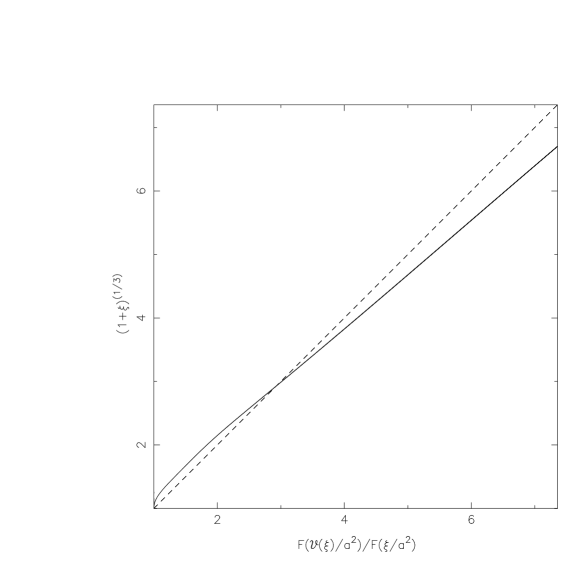
Figure 1: The approximate solution to the functional equation determining the pseudo-linear profile is plotted. See text for discussion.

This approximate profile works reasonably well. Figures 1 and 2 show this result. In figure 1 we have plotted the ratio $F({\cal V}(\bar{\xi})/{a^{2}})/F({\bar{\xi}}/{a^{2}})$ on the x-axis and the function $(1+\bar{\xi})^{1/3}$ on the y-axis. If the function in (56) satifies equation (42) exactly, we should get a 45-degree line in the figure which is shown by a dashed line. The fact that our curve is pretty close to this line shows that the ansatz in (56) satisfies equation (42) fairly well. The optimum value of $B$ chosen for this figure is $B=38.6$. When $a$ is varied from $1$ to $10^{3}$, the percentage of error between the 45-degree line and our curve is less than about 20 percent in the worst case. It is clear that our profile in (56) satisfies equation (57) quite well for a dynamic range of $10^{6}$ in $a^{2}$.

Figure 2 shows this result more directly. We evolve the pseudo linear profile form $a^{2}=1$ to $a^{2}\approx 1000$ using the NSR, and plot $[\bar{\xi}(a,x)/a^{2}]$ against $x$. The dot-dashed, dashed and two solid curves (upper one for $a^{2}=100$ and lower one for $a^{2}=900$) are for $a^{2}=1,9,100$ and $900$ respectively. The overlap of the curves show that the profile does grow approximately as $a^{2}$. Also shown are lines of slope $-1$ (dotted) and $-2$ (solid); clearly $\bar{\xi}\propto x^{-1}$ for small $x$ and $\bar{\xi}\propto x^{-2}$ in the intermediate regime.

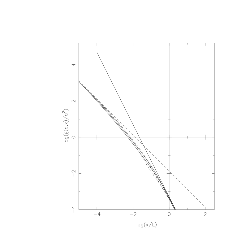
Figure 2: The dot-dashed,dashed and two solid curves (upper one for $a^{2}=100$ and lower one for $a^{2}=900$) are for $a^{2}=1,9,100$ and $900$. The dotted straight line is of slope -1 and the solid one is of slope-2 showing both the $1/x$ and $1/x^{2}$ regions of the profile

We emphasis that we have chosen in equation (56) the simplest kind of ansatz combining the two regimes and we have used only two parameters $A$ and $B$. It is quite possible to come up with more elaborate fitting functions which will solve our functional equation far more accurately but we have not bothered to do so for two reasons: (i) Firstly, the fitting functions in equation (11) for ${\cal V}(z)$ itself is approximate and is probably accurate only at 10-20 percent level. There has also been repeated claims in literature that these functions have weaker dependence on $n$ which we have ignored for simplicity in this paper. (ii) Secondly, one must remember that only those $\bar{\xi}$ which correspond to positive definite $P(k)$ are physically meaningful. This happens to be the case our choice [which can be verified by explicit numerical integration with a cutoff at large $x$] but this may not be true for arbitrarily complicated fitting functions. Incidentally, another simple fitting function for the pseudo-linear profile is

$$\bar{\xi}(a,x)=a^{2}\frac{A^{\prime}}{(x/L^{\prime})[(x/L^{\prime})+1]}$$ (58)

with $A^{\prime}=B^{2}$ and $L^{\prime}=L/4$.

If a more accurate fitting is required, one can obtain it more directly from equation (16). Setting $n_{a}=2$ in that equation predicts the instantaneous spatial slope of $\bar{\xi}(a,x)$ to be

$$\frac{\partial\ln\bar{\xi}(a,x)}{\partial\ln x}=\frac{2}{h[\bar{\xi}(a,x)]}-3(1+\frac{1}{\bar{\xi}(a,x)})$$ (59)

which can be integrated to give

$$\ln\frac{x}{L}=\int_{\bar{\xi}[L]}^{\bar{\xi}[x]}\frac{hd\bar{\xi}}{\bar{\xi}(2-3h)-3h}$$ (60)

at $a=1$ with $L$ being an arbitratry integration constant. Numerical integration of this equation will give a profile which is varies as $(1/x)$ at small scales and goes over to $(1/x^{2})$ and then to $(1/x^{3}),(1/x^{4})....$ etc with an asymptotic logarithmic dependence. In the regime $\bar{\xi}(a,x)>1$, this will give results reasonably close to our fitting function.

It should be noted that equation (42) reduces to an identity for any $F$, in the limit $\bar{\xi}\to 0$ since, in this limit ${\cal V}(z)\approx z$. This shows that we are free to modify our pseudo-linear profile at large scales into any other form [essentially determined by the input linear power spectrum] without affecting any of our conclusions.

Finally, we will discuss a different way of thinking about pseudolinear profiles which may be useful.

In studying the evolution of the density contrast $\delta(a,{\bf x})$, it is conventional to expand in in term of the plane wave modes as

$$\delta(a,{\bf x})=\sum_{\bf k}\delta(a,{\bf k})\exp(i{\bf k}\cdot{\bf x})$$ (61)

In that case, the exact equation governing the evolution of $\delta(a,{\bf k})$ is given by (Peebles (1980))

$$\frac{d^{2}\delta_{\bf k}}{da^{2}}+\frac{3}{2a}\frac{d\delta_{\bf k}}{da}-\frac{3}{2a^{2}}\delta_{\bf k}={\cal A}$$ (62)

where ${\cal A}$ denotes the terms responsible for the nonlinear coupling between different modes. The expansion in equation (61) is, of course, motivated by the fact that in the linear regime we can ignore ${\cal A}$ and each of the modes evolve independently. For the same reason, this expansion is not of much value in the highly nonlinear regime.

This prompts one to ask the question: Is it possible to choose some other set of basis functions $Q(\alpha,{\bf x})$, instead of $\exp\;i{\bf k}\cdot{\bf x}$, and expand $\delta(a,{\bf x})$ in the form

$$\delta(a,{\bf x})=\sum_{\alpha}\delta_{\alpha}(a)\;Q(\alpha,{\bf x})$$ (63)

so that the nonlinear effects are minimised ? Here $\alpha$ stands for a set of parameters describing the basis functions. This question is extremely difficult to answer, partly because it is ill-posed. To make any progress, we have to first give meaning to the concept of “minimising the effects of nonlinearity”. One possible approach we would like to suggest is the following: We know that when $\delta(a,{\bf x})\ll 1$,then $\delta(a,{\bf x})\propto a\>F({\bf x})$ for any arbitrary $F({\bf x})$; that is all power spectra grow as $a^{2}$ in the linear regime. In the intermediate and nonlinear regimes, no such general statement can be made. But it is conceivable that there exists certain special power spectra for which $P({\bf k},a)$ grows (at least approximately) as $a^{2}$ even in the nonlinear regime. For such a spectrum, the left hand side of (62) vanishes (approximately); hence the right hand side should also vanish. Clearly, such power spectra are affected least by nonlinear effects. Instead of looking for such a special $P(k,a)$ we can, equivalently look for a particular form of $\bar{\xi}(a,x)$ which evolves as closely to the linear theory as possible. Such correlation functions and corresponding power spectra [which are the pseudo-linear profiles] must be capable of capturing most of the essence of nonlinear dynamics. In this sense, we can think of our pseudo-linear profiles as the basic building blocks of the nonlinear universe. The fact that the correlation function is closely related to isothermal spheres, indicates a connection between local gravitational dynamics and large scale gravitational clustering.

6 Conclusions

It seems reasonable to hope that the late stage evolution of collisionless point particles, interacting via newtonian gravity in an expanding background, should be understandable in terms of a simple paradigm. This paper [ as the title implies! ] tries to realise this dream within some well defined framework. It should be viewed as a tentative first step in a new direction which seems promising.

There are three key points which emerge from this analysis. The first is the fact that we have been able to find approximate correlation functions which evolve preserving their shapes. We achieved this by looking at the structure of an exact equation which obeys certain nonlinear scaling relations. As we emphasised before, the existence of such special class of solutions to the equations of gravitational dynamics is an important feature.

Secondly, we should take note of the role played by the “isothermal” profile $(1/x^{2})$ in our solution. Such a profile can lead to correlation functions which go as $(1/x)$ at small scales and $(1/x^{2})$ in the intermediate scales. If this profile is indeed “special” then one expects it to lead to a pseudo-linear profile for the correlation function. Our analysis shows that there is indeed good evidence for this feature. If one accepts this evidence, then the next level of enquiry would be to ask why $(1/x^{2})$ profiles are “special”. In the statistical mechanics of gravitating systems, one can show that these profiles arise as end stages of violent relaxation which operates at dynamical time scales. Whether a similar reasoning holds in an expanding background, independent of the index for power spectrum, is open to question. This is an important issue and we hope to address it fully in a future work. We emphasise that our equations, along with NSR, naturally lead to a pseudo-linear profile, which can be interpreted and understood in terms of isothermal density profiles for halos; we did not have to assume anything a priori regarding the halo profiles.

In a more pragmatic way, one can understand the pseudo-linear profile from the dependence of the rate of growth of the correlation function on the local slope. The NSR suggest that $\bar{\xi}$ grows (approximately) as $a^{6/(n_{eff}+4)}$ in the intermediate regime and as $a^{6/(n_{eff}+5)}$ in the nonlinear regime. This scaling shows that $n_{eff}=-1$ grows as $a^{2}$ in the intermediate regime and $n_{eff}=-2$ grows as $a^{2}$ in the nonlinear regime. This is precisely the form our pseudo-linear profile has. Also, in the intermediate regime, the correlation grows faster than $a^{2}$ if $n_{eff}<-1$ and slower than $a^{2}$ if $n_{eff}>-1$. The net effect is, of course, to straighten out a curved correlation and drive it to $n=-1$. Similar effect drives the correlations to $n=-2$ in the nonlinear regime.[see Bagla & Padmanabhan (1997) for a more detailed discussion of this aspect in the intermediate regime]. Of course, one still needs to understand the dependence of growth rate on the $n_{eff}$ from more physical considerations to get the complete picture. We have not addressed in this paper, what is the timescale over which clustering can lead to the psuedo-linear profile even granting that it does. This requires further study.

The last aspect has to do with what one can achieve using the pseudo-linear profiles. In principle, one would like to build the nonlinear density field through a superposition of pseudo-linear profiles but this is a mathematically complex problem. As a first step one should understand why the nonlinear term in equation (62) is subdominant for such a profile. This itself is complicated since we have only fixed the power spectrum — but not the phases of the density modes — while the nonlinear terms do depend on the phase. Again, we hope to investigate this issue further in a future work.

References

- Bagla & Padmanabhan (1997) Bagla J.S and Padmanabhan T., MNRAS, 1997, in press
- Hamilton et al. (1991) Hamilton A.J.S., Kumar P., Lu E. and Mathews A., 1991, ApJ, 374, L1
- McClelland & Silk (1977) McClelland J. and Silk, J., 1977, ApJ, 217, 331
- Mo, Jain & White (1995) Mo H.J.,Jain B. and White S.M.,1995, MNRAS,276,L25
- Navarro, Frenk & White (1996) Navarro J.F, Frenk C.S and White S.D.M 1996, Ap.J,462,563
- Nityananda & Padmanabhan (1994) Nityananda R. and Padmanabhan T, 1994,MNRAS,271,976
- Padmanabhan (1990) Padmanabhan T., 1990, Physics Reports,188,285
- Padmanabhan (1996) Padmanbhan T., 1996, MNRAS,278, L29
- (9) Padmanabhan, T., 1996 a, Cosmology and Astrophysics - through problems, Cambridge University Press, Cambridge, p.410
- Padmanabhan et al. (1996) Padmanabhan T., Cen R., Ostriker J.P. and Summers F.J., 1996, ApJ, 466, 604
- Peacock & Dodds (1994) Peacock J.A and Dodds S.J., 1994, MNRAS, 267, 1020
- Peacock & Dodds (1996) Peacock J.A and Dodds S.J., 1996, MNRAS, 280, L19
- Peebles (1980) Peebles P.J.E., 1980, Large Scale Structure of the Universe, Princeton Univ. Press, Princeton, NJ
- Sheth & Jain (1997) Sheth R. and Jain B., 1997, MNRAS,285 231