Molecular Hydrogen in Diffuse Interstellar Clouds
of Arbitrary Three-Dimensional Geometry

Abstract

We have constructed three-dimensional models for the equilibrium abundance of molecular hydrogen within diffuse interstellar clouds of arbitrary geometry that are illuminated by ultraviolet radiation. The position-dependent photodissociation rate of H₂ within such clouds was computed using a 26-ray approximation to model the attenuation of the incident ultraviolet radiation field by dust and by H₂ line absorption.

We have applied our modeling technique to the isolated diffuse cloud G236+39, assuming that the cloud has a constant density and that the thickness of the cloud along the line of sight is at every point proportional to the 100 $\mu$m continuum intensity measured by IRAS. We find that our model can successfully account for observed variations in the ratio of 100 $\mu$m continuum intensity to HI column density, with larger values of that ratio occurring along lines of sight in which the molecular hydrogen fraction is expected to be largest.

Using a standard $\chi^{2}$ analysis to assess the goodness of fit of our models, we find (at the 60$\sigma$ level) that a three-dimensional model is more successful in matching the observational data than a one-dimensional model in which the geometrical extent of the cloud along the line of sight is assumed to be very much smaller than its extent in the plane-of-the-sky. If $D$ is the distance to G236+39, and given standard assumptions about the rate of grain-catalysed H₂ formation, we find that the cloud has an extent along the line of sight that is $0.9\pm 0.1$ times its mean extent projected onto the plane of the sky; a gas density of $(53\pm 8)\,(100\,{\rm pc}/D)$ H nuclei per cm³; and is illuminated by a radiation field of $(1.1\pm 0.2)\,(100\,{\rm pc}/D)$ times the mean interstellar radiation field estimated by Draine (1978). The derived 100 $\mu$m emissivity per nucleon is $(1.13\pm 0.06)\times 10^{-20}\rm\,MJy\,sr^{-1}cm^{2}$.

1 Introduction

Diffuse interstellar clouds of visual extinction $A_{\rm V}\sim 1$ mag represent the intermediate case between atomic clouds in which the molecular fraction is very small and dense molecular clouds in which gas is almost fully molecular; as such, they represent the best laboratories in which to study the formation and destruction of molecular hydrogen.

1.1 Observations of molecular hydrogen in diffuse clouds

Direct observations of molecular hydrogen in diffuse molecular clouds have been severely hampered by the absence of any dipole-allowed transitions at radio, infrared or visible wavelengths. Given current instrumental sensitivities, direct measurements of the H₂ abundance in diffuse clouds can only be obtained from observations of the dipole-allowed electronic transitions of the Lyman and Werner bands. These transitions, which lie in the $912-1100$ Å spectral region, were detected by the Copernicus satellite in absorption toward more than one hundred background sources (Spitzer et al. 1973; Savage et al. 1979). Although the planned Far Ultraviolet Spectroscopic Explorer (FUSE) will allow such absorption line studies to be carried out toward fainter background sources than those observed with Copernicus, direct observations of molecular hydrogen will continue to allow only sparse spatial sampling of diffuse molecular clouds.

An alternative – although less direct – means of studying the distribution of H₂ in diffuse molecular clouds is afforded by the combination of HI 21cm observations and 100 $\mu$m continuum observations carried out by the IRAS satellite. The diffuse cloud that has been studied most extensively by this method is G236+39, an isolated high-latitude cloud (Galactic coordinates $b=38.23$, $l=235.73$) of angular size $\sim 2\times 1$ degrees for which Reach, Koo & Heiles (1994) have used the Arecibo radio telescope to obtain a complete HI map at a spatial resolution (3 arcminutes) comparable to that of the IRAS beam ($3\times 5$ arcminutes). Given the absence of any stellar sources associated with G236+39, the distance is unfortunately not well determined. Figure 1, based upon data kindly provided in electronic form by W. Reach, shows the HI column densities, $N({\rm HI})$, and 100 $\mu$m continuum intensities, $I_{100}$, for more than 4000 lines of sight toward this cloud. Assuming that $I_{100}$ is linearly proportional to the column density of H nuclei, $N_{\rm H}=N({\rm HI})+2\,N({\rm H_{2}})$, Reach et al. argued that the higher ratios of $I_{100}/N({\rm HI})$ typically observed when $N({\rm HI})$ is large represented the effects of molecule formation along the line of sight. This allowed the H₂ column density to be estimated as $N({\rm H_{2}})=0.5\,[(I_{100}/r_{0})-N({\rm HI})]$, where $r_{0}=I_{100}/N_{\rm H}$ is the 100 $\mu$m emission coefficient per H nucleus, a quantity that could be determined from the slope of the $I_{100}$ versus $N({\rm HI})$ correlation in the small column density limit where the molecular fraction was negligible.

1.2 Models of diffuse clouds

The chemistry of diffuse molecular clouds has been the subject of extensive theoretical study over the past 25 years (e.g. Black & Dalgarno 1977; van Dishoeck & Black 1986; Spaans 1996, and references therein). Common to all theoretical models for diffuse molecular clouds are the assumptions that the formation of molecular hydrogen takes place by means of grain surface reactions and that the destruction of H₂ occurs primarily by photodissociation. Because photodissociation of H₂ follows line absorption of ultraviolet radiation in the Lyman and Werner bands, the photodissociation rate is diminished by self-shielding and shows a strong depth-dependence.

Most previous studies of diffuse cloud chemistry have assumed a one-dimensional plane-parallel geometry, in which a geometrically-thin slab is illuminated by ultraviolet radiation from either one or two sides. The solid curve in Figure 1 shows the predicted variation of $I_{100}$ with $N({\rm HI})$ for a series of slab models illuminated from two sides with a constant assumed density of H nuclei and a variable column density. As described in §3 below, the assumed 100$\mu$m emissivity per H nucleus and the cloud density have been chosen to optimize the fit to the data. In the limit of small $N({\rm HI})$, the predicted relationship between $I_{100}$ and $N({\rm HI})$ is linear, but for $N({\rm HI})\geq\rm few\,\times 10^{20}cm^{-3}$, the molecular hydrogen fraction becomes significant and the curve turns upwards.

While a one-dimensional slab model can evidently account for the gross properties of the data plotted in Figure 1, we have investigated in this study whether a better fit to the data can be obtained with models in which a three-dimensional cloud structure is assumed. Thus instead of modeling the cloud G236+39 as a “cardboard cutout” that has an extent along the line of sight that is very much smaller than its extent in the plane-of-the-sky, we have constructed a series of three-dimensional models in which we assume the cloud to have a significant geometrical thickness perpendicular to the plane of the sky. In other words, we include the photodissociative effects of radiation that is incident upon the cloud from the sides as well as along the line of sight.

This paper is organized as follows. In §2 we describe the numerical method used to model the formation and dissociation of H₂ in a three-dimensional diffuse cloud of arbitrary shape. In §3 we investigate whether our three-dimensional models describe more accurately than one-dimensional models the correlation between IRAS 100 $\mu$m emission and HI column density for the line of sight toward the cirrus cloud G236+39. The results of our investigation are discussed in §4.

2 Computational Method

We have constructed a model for the equilibrium H₂ abundance within a three-dimensional molecular cloud with a constant density of H nuclei and an arbitrary shape. This study extends the spherical cloud models described by Neufeld & Spaans (1996).

We assume that molecular hydrogen is formed catalytically on dust grains at a rate $R\,n_{\rm H}n({\rm HI})$ per unit volume, where $n({\rm HI})$ is the density of hydrogen atoms, $n_{\rm H}=n({\rm HI})+2\,n({\rm H_{2}})$ is the density of hydrogen nuclei, and $R=3\times 10^{-17}\,\alpha\,\rm cm^{3}\,s^{-1}$ is an effective rate coefficient with a “canonical value” of $3\times 10^{-17}\rm cm^{3}\,s^{-1}$ (Jura 1974) corresponding to $\alpha=1$.

The destruction of H₂ is dominated by spontaneous radiative dissociation, following the absorption of 912–1110 Å ultraviolet radiation in the Lyman and Werner bands. Given the estimate of Draine (1978) for the mean UV interstellar radiation field, and the Lyman and Werner band oscillator strengths and photodissociation probabilities of Allison & Dalgarno (1970) and Stephens & Dalgarno (1972), the photodissociation rate for an unshielded H₂ molecule is $\zeta_{0}=5.0\times 10^{-11}\rm\,s^{-1}$. Once the Lyman and Werner transitions become optically-thick, the photodissociation rate is diminished due to self-shielding. In modeling the decrease of the photodissociation rate due to self-shielding along any given ray, we adopt the expression given by Tielens & Hollenbach (1985) for the self-shielding function for spectral lines with a Voigt profile. We assume that dust absorption decreases the photodissociation rate further by a factor $\exp(-2.55A_{\rm V})$, where $A_{\rm V}$ is the visual extinction along the ray. The value for the exponent, $-2.55A_{\rm V}$, is based upon the opacity, albedo and scattering behavior of interstellar grains given by Roberge et al. (1991), and has been verified with the spherical harmonics method of Roberge (1983) for a plane-parallel slab and with the Monte Carlo code of Spaans (1996) for a sphere.

With these assumptions, the H₂ photodissociation rate, $\zeta$, at an arbitrary point P within the cloud may be written

$${\zeta\over\zeta_{0}}={1\over 4\pi}\int I_{UV}({\bf{\hat{k}}})\,f(N[{\rm H}_{2},{\bf{\hat{k}}}])\,\exp(-2.55\,A_{\rm V}[{\bf{\hat{k}}}])d\Omega,$$

where $N[{\rm H}_{2},{\bf{\hat{k}}}]$ is the column density of H₂ molecules along direction ${\bf{\hat{k}}}$ from the cloud surface to point P, $A_{\rm V}[{\bf{\hat{k}}}]$ is the visual extinction along the same path, $f(N)$ is the H₂ self-shielding function, and $I_{UV}({\bf{\hat{k}}})$ is the incident ultraviolet intensity in direction $({\bf{\hat{k}}})$ in units of the mean interstellar radiation field given by Draine (1978). In the absence of any reliable distance estimate for the cloud to which our computational method will be applied (G236+39), we have no means of estimating the angular dependence of $I_{UV}$. We therefore make the simplest assumption that the ultraviolet radiation field is isotropic, $I_{UV}({\bf{\hat{k}}})=I_{UV}$. The equilibrium H₂ abundance at point P is given by

$${n({\rm H}_{2})\over n_{\rm H}}={R\,n_{H}\over\zeta+2\,R\,n_{H}}.$$

The H₂ abundance is a decreasing function of the parameter $I_{UV}/(\alpha n_{\rm H})$, which characterizes the relative rates of H₂ photodissociation and H₂ formation.

In our computer model for the formation and photodissociation of H₂ in three-dimensional clouds, the angular integration in equation (1) was performed using a 26-ray approximation. Here the angular integration was discretized on a grid of 26 directions, described in Cartesian coordinates by the k-vectors $(x,y,z)$ with $x$, $y$, and $z$ taking any of the values –1, 0, or 1. The H₂ abundance was computed at every point using equations (1) and (2). Since the shielding column densities $N[{\rm H}_{2},{\bf{\hat{k}}}]$ that enter equation (1) depend upon the molecular abundances obtained in equation (2), an iterative method was used to obtain a simultaneous solution, with the convergence criterion that the change in H₂ abundance between successive iterations was everywhere less than 1%.

To verify the accuracy of our computer code, one-dimensional plane-parallel slab calculations were performed and compared with results obtained from the 1-D computer code of Black & van Dishoeck (1987). Figure 2 shows a representative computation for a model slab with $T=50$ K, $I_{\rm UV}=3$, $n_{\rm H}=200$ cm^-3 and $A_{\rm V}=1$ mag. The predicted H₂ abundances agree to within 2%.

3 The IRAS Cloud G236+39

The IRAS cloud G236+39 is an isolated, high latitude ($b=38.23$) cirrus cloud that provides an excellent test case in which our three-dimensional diffuse cloud models can be assessed. The absence of any stellar sources associated with G236+39 causes the distance to be not well determined.

3.1 Assumed geometry

As described in §1 above, Reach et al. (1994) have used the Arecibo radiotelescope to map the HI 21cm line emission from G236+39 at an angular resolution of 3 arcminutes, yielding estimates of the HI column density along 4421 lines of sight through this cloud. We obtained estimates of the IRAS 100 $\mu$m continuum intensity radiated by G236+39 along the same lines of sight, using the IRSKY facility made available by IPAC to estimate and subtract the 100 $\mu$m background.

We then interpreted the background-subtracted 100 $\mu$m intensity map as a “topographical contour map” of the cloud, assuming that the intensity at each position is proportional to the spatial extent of the cloud along the line of sight. Two critical assumptions underlie this interpretation: we assume (1) that the 100 $\mu$m intensity is linearly proportional to the column density of H nuclei (Boulanger & Pérault 1988), i.e. that $I_{100}=r_{0}\,N_{\rm H}$ with $r_{0}$ constant; and (2) that the density of H nuclei within the cloud, $n_{\rm H}$, is also constant. With these assumptions, the linear extent along the line of sight is $I_{100}/(r_{0}n_{\rm H})$. Both the assumptions of constant $r_{0}$ and of constant $n_{\rm H}$ are plausible for a diffuse cloud such as G236+39. In general, we expect $r_{0}$ to increase with increasing depth into a cloud because the ultraviolet radiation that heats the dust responsible for the 100 $\mu$m continuum emission is itself attenuated by dust absorption. However, the extinction to the center of G236+39 is relatively small ($A_{\rm V}\sim 0.3$ mag), and the absence of any correlation between the $\rm 60\mu m/100\mu m$ intensity ratio and the 100 $\mu$m intensity argues against any significant variation in the dust temperature (and thus in $r_{0}$) within the cloud (Reach et al. 1994). Similarly, considerations of hydrostatic equilibrium imply that the cloud is only slightly self-gravitating so that the pressure is not expected to vary significantly within the cloud. Since the total pressure in diffuse clouds is dominated by microturbulent rather than thermal motions (van Dishoeck & Black 1989; Crawford & Barlow 1996), and since there is no evidence for significant gradients in the microturbulent line widths, the absence of significant variations in the pressure implies that the total mass density (or equivalently, the density of H nuclei, $n_{H}$ is roughly constant).

Our assumption that the 100 $\mu$m intensity at each position is proportional to the spatial extent of the cloud along the line of sight does not determine the three-dimensional shape of the cloud uniquely. Because the 100 $\mu$m intensity measures only the extent of the cloud along the line of sight but not its location, a given 100 $\mu$m map is consistent with a whole set of cloud shapes that are related by shears perpendicular to the plane of the sky. Thus we specify a unique cloud shape be making the additional (and admittedly arbitrary) assumption that the cloud possesses reflection symmetry about the plane of the sky.

While all our three-dimensional models for G236+39 are based upon the assumption that the cloud thickness along the line of sight is proportional to the measured 100 $\mu$m intensity, we have varied the constant of proportionality in that relationship so as to obtain the best fit to the data. Each model may be characterized conveniently by an elongation factor $F_{E}$ which describes the degree of elongation along the line of sight:

$$F_{E}\equiv{\sqrt{3\pi}\over 4}{t_{\rm max}\over A^{1/2}},$$

where $t_{\rm max}=I_{100}[{\rm max}]/(r_{0}n_{\rm H})$ is the maximum assumed thickness of the cloud, $I_{100}[{\rm max}]$ is the maximum 100 $\mu$m intensity, and $A$ is the projected area of the half-maximum intensity contour, $I_{100}=0.5\,I_{100}[{\rm max}]$. The factor $\sqrt{3\pi}/4$ has been introduced so that the elongation factor $F_{E}$ is defined as unity for the case of a sphere; elongation factors smaller than unity then apply to oblate shapes that are flattened along the line of sight while elongation factors greater than unity apply to prolate shapes that are elongated along the line of sight. In this notation, the one-dimensional geometry traditionally used to model molecular clouds is described by the limiting case $F_{E}=0$.

For G236+39, the angular area of the half-maximum 100 $\mu$m intensity contour is $7.6\times 10^{-5}\rm\,sr$, corresponding to a physical area $A=9.1\times 10^{37}\,(D/\rm 100\,pc)^{2}\,cm^{2}$ for an assumed distance to the source of $D$. The elongation factor is then related to the density $n_{\rm H}$ by the expression

$$F_{E}=0.56\,\biggl{(}{10^{-20}{\rm MJy\,sr^{-1}cm^{2}}\over r_{0}}\biggr{)}\,\biggl{(}{{\rm 100\,pc}\over D}\biggr{)}\,\biggl{(}{{\rm 100\,cm^{3}}\over n_{\rm H}}\biggr{)}.$$

3.2 $\chi^{2}$ analysis

Given the observed IRAS 100 $\mu$m map for G236+39, the molecular fraction can be predicted at every point in the cloud using the methods described in §2 above. The results depend upon three parameters: the 100 $\mu$m emission coefficient per H nucleus, $r_{0}$; the elongation factor, $F_{E}$; and the quantity $I_{UV}/(\alpha n_{\rm H})$, which represents the relative rates of H₂ photodissociation and H₂ formation (see §2 above). Once predictions have been obtained for the H₂ abundance everywhere in the cloud, a predicted HI column density map can be obtained by integrating $n({\rm H})=n_{\rm H}-0.5\,n({\rm H}_{2})$ along each line of sight.

We use a standard $\chi^{2}$ analysis to compare the predicted HI map with the observations of Reach et al. (1994) and thereby to constrain the values of $r_{0}$, $F_{E}$, and $I_{UV}/(\alpha n_{\rm H})$. Assuming that the HI observations have a fractional error that is roughly the same for each line of sight (Reach et al. 1994), the $\chi^{2}$ parameter is proportional to the sum

$$S=\sum\biggl{[}(N_{\rm obs}/N_{\rm com})-1\biggr{]}^{2}$$

over all lines of sight, where $N_{\rm obs}$ is the observed HI column density and $N_{\rm com}$ is the computed (i.e. predicted) value.

To assess whether three-dimensional (i.e. $F_{E}>0$) models for G236+39 are superior to one-dimensional ($F_{E}=0$) models, we have constructed a series of models of increasing elongation factor, $F_{E}$. For each such model, we have varied the other parameters, $r_{0}$ and $I_{UV}/(\alpha n_{\rm H})$, so as to minimize $\chi^{2}$. Figure 3 shows the smallest value of $\chi^{2}$ that can be achieved for fixed elongation factor, as a function of $F_{E}$, relative to the minimum value that can be achieved for any elongation factor, $\chi^{2}_{\rm min}$.

Figure 3 shows clearly that the global minimum in $\chi^{2}$ is obtained for non-zero $F_{E}$. The best estimate of $F_{E}$ is 0.9, and the standard error on that estimate is 0.1. Given the statistical properties of the $\chi^{2}$ parameter, the results show at the $60\sigma$ level that a three-dimensional model with $F_{E}=0.9$ provides a better fit to the data than a one-dimensional ($F_{E}=0$) model.

The comparison between the 3-D ($F_{E}=0.9$) and 1-D ($F_{E}=0$) models can be illustrated graphically in at least three other ways. In Figure 4, we show the histogram of $N_{\rm obs}/N_{\rm com}$ values for all 4421 lines of sight; the 3-D model clearly yields a narrower distribution. Figure 5 shows the values of $N_{\rm obs}/N_{\rm com}$ as a function of $N_{\rm obs}$. Again, the 3-D model (upper panel) clearly shows a tighter fit to the data, and another feature of the results becomes apparent: the 1-D model (lower panel) systematically underpredicts the HI column density (i.e. overpredicts the molecular fraction) when $N({\rm HI})\sim 3-5\times 10^{20}\rm cm^{-2}$ and overpredicts the HI column density when $N({\rm HI})\sim 5-8\times 10^{20}\rm cm^{-2}$. This behavior is also exhibited by the false color figures displayed in Plate 1. Here the two left panels show the value of $N_{\rm obs}/N_{\rm com}$ for every line of sight toward G236+39, the upper left panel applying to the 1-D model and the lower left panel to the 3-D model. Values of $N_{\rm obs}/N_{\rm com}$ close to unity appear green in this figure while values greater than unity appear yellow or red and values smaller than unity appear blue or violet. Again, the 3-D model yields a better fit to the data, and the 1-D model shows a systematic tendency to underestimate the HI column density (and overestimate the molecular fraction) near the edges of the cloud, where the HI column density lies in the range $3-5\times 10^{20}\rm cm^{-2}$. This tendency arises because the 1-D model does not include the photodissociative effects of radiation propagating in the plane of the sky; near the edges of the cloud, such radiation is attenuated by an H₂ column density that is considerably less than the column density along the line of sight, so the 1-D model significantly underestimates the photodissociation rate. The right hand panels in Plate 1 compare the observed ratio of the 100 $\mu$m continuum intensity to the HI column density (lower right panel) with the predicted ratios for the best fit 3-D model (middle right panel) and the best fit 1-D model (upper right panel). The ratio of the 100 $\mu$m continuum intensity to the HI column density is a measure of the mean molecular fraction along the line of sight; once again, the 3-D model clearly provides a better fit.

3.3 Derived cloud parameters

The parameters derived for the best fit 1-D model (with the elongation factor $F_{E}$ fixed at zero) and the best fit 3-D model (with $F_{E}$ taking whatever value optimizes the fit to the data) are tabulated in Table 1. Even the 3-D models do not completely determine the cloud parameters, because the $\chi^{2}$ analysis places constraints upon three variables ($r_{0}$, $F_{E}$, and $I_{UV}/[\alpha n_{H}]$) whereas the total number of unknown parameters is five ($r_{0}$, $I_{UV}$, $n_{\rm H}$, $\alpha$ and $D$). Adopting “canonical values” for the ultraviolet radiation field ($I_{UV}=1$) and for the H₂ formation rate coefficient ($\alpha=1$), we obtain estimates of $(1.13\pm 0.06)\times 10^{-20}\rm\,MJy\,sr^{-1}cm^{2}$ for the 100 $\mu$m emission coefficient per H nucleus, $r_{0}$; $(48\pm 7)\rm\,cm^{-3}$ for the density of H nuclei, $n_{\rm H}$; and $(110\pm 20)$ pc for the distance to the source, $D$. (All the error bounds given here are $1\sigma$ statistical uncertainties.) Figure 6 shows the three-dimensional shape of the cloud G236+39 that is implied by the elongation factor that we derived.

4 Discussion

The $\chi^{2}$ analysis described in §3.2 above establishes convincingly that the abundance of H₂ in G236+39 is explained more successfully by a 3-D model than by a 1-D model. Furthermore, the 3-D model provides a distance estimate of $D\sim 100$ pc which is at least consistent with the known scale height of cold HI in the Galaxy.

4.1 Validation of the model

As a further test of our method, we have applied it to a set of artificial 100 $\mu$m and HI 21 cm maps that we generated for the case of a triaxial spheriod of elongation factor unity. After adding artificial noise to those maps, we attempted to reconstruct the elongation factor for that spheriod using a $\chi^{2}$ analysis exactly analogous to that described in §3.2. The elongation factor was indeed recovered successfully, the derived value being $1.02\pm 0.06\,\,(1\sigma)$. Full details of this analysis and figures analogous to those described in §3 are presented in the Appendix.

4.2 Limitations of the model

Despite its apparent success in providing a better fit to the observational data than a 1-D model, our 3-D model is clearly idealized in that we have made several simplifying assumptions. The assumptions of constant $n_{\rm H}$ and $r_{0}$ have already been discussed in §3.1 above. Our assumption that the cloud G236+39 shows reflection symmetry about the plane of the sky has also been discussed; because we assume that all the low-level 100 $\mu$m emission near the edges of the cloud arises from material that is located close to the symmetry plane, this assumption probably leads to an overestimate of the degree of shielding at the cloud center. A further simplifying assumption is our adoption of an isotropic incident radiation field.

We have also assumed that the H₂ chemistry is in equilibrium, with the rate of photodissociation equal to the rate of formation. The timescale for establishing such a chemical equilibrium is $\tau_{\rm chem}=1/(Rn_{\rm H})\sim 20\rm\,Myr$. (Note that the estimate given by Reach et al. 1994 is too large by an order of magnitude.) For comparison, we may define a crossing timescale as the ratio of the cloud size to the HI linewidth, $\tau_{\rm cross}=I_{100}[{\rm max}]/(n_{\rm H}r_{0}\Delta v)\sim 3\rm\,Myr$, where $\Delta v\sim 3\rm\,km\,s^{-1}$ is the typical HI linewidth. The fact that $\tau_{\rm chem}$ exceeds $\tau_{\rm cross}$ does not necessarily invalidate our assumption of chemical equilibrium. Even assuming that turbulent motions contribute significantly to the line width, we would expect that turbulent mixing will tend to decrease the molecular fraction in the cloud interior only if $\tau_{\rm chem}$ also exceeds the turbulent diffusion timescale, $\tau_{\rm diff}$, which we expect to be larger than $\tau_{\rm cross}$ by the ratio of the cloud size to the effective mixing length. Turning the argument around, we suggest that the success of our equilibrium models in explaining the observations implies that $\tau_{\rm diff}$ is indeed long relative to $\tau_{\rm chem}$ and that the ratio of the cloud size to the effective mixing length is greater than $\sim 10$.

4.3 Future studies of H₂ in diffuse molecular clouds

We anticipate several future extensions to the study presented in this paper. Thus far, we have only applied our 3-D modeling methods to the single source G236+39; one obvious extension will be their application to other isolated diffuse clouds. In addition, we expect that observations at other wavelengths will provide useful additional probes of the physical and chemical conditions in diffuse clouds such as G236+39. In particular, CII fine structure emissions in the $\rm{}^{3}P_{3/2}-^{3}P_{1/2}$ line near 158 $\mu$m would provide a valuable independent probe of the density and a check on our assumption that $n_{\rm H}$ is roughly constant. Except at the cloud center, from which CO emissions have been detected (Reach et al. 1994), we expect C⁺ to be the dominant reservoir of gas-phase carbon nuclei in G236+39; thus C⁺ will have a roughly constant abundance relative to H nuclei. Because the density in diffuse clouds is very much smaller than the critical density for the CII $\rm{}^{3}P_{3/2}-^{3}P_{1/2}$ transition, the frequency-integrated CII line intensity will therefore be proportional to $N_{\rm H}n_{\rm H}$, and the CII line equivalent width will be proportional to $n_{\rm H}$. The Infrared Space Observatory (ISO), the Stratospheric Observatory for Infrared Astronomy (SOFIA), as well as planned balloon-borne telescopes will provide ideal platforms for carrying out CII observations of diffuse clouds. We note that only a relatively small telescope (with a 20 cm diameter primary mirror) is needed to provide a beam size at 158 $\mu$m that matches the beam size of the Arecibo radiotelescope for H 21 cm observations.

The far ultraviolet is another spectral region that is important for the study of molecular hydrogen in diffuse clouds. In particular, the launch of the Far Ultraviolet Spectroscopic Explorer will permit the direct measurement of H₂ column densities in absorption along specific lines of sight toward ultraviolet continuum sources. Although the spatial sampling provided by such absorption line studies will be limited by the availability of bright background sources, FUSE observations will provide a very valuable complement to the indirect methods for studying H₂ that have been described in this paper.

We are very grateful to W. Reach for making available the H 21cm map of G236+39, and to E. van Dishoeck for allowing us to use her computer code as a check on our results in the limit $F_{E}=0$. We acknowledge with gratitude the support of NASA grant NAGW-3147 from the Long Term Space Astrophysics Research Program. Most of the simulations presented in this work were performed on the Cray Y-MP operated by the Netherlands Council for Supercomputer Facilities in Amsterdam.

APPENDIX

As a further test of our method, we have applied it to a set of artificial 100 $\mu$m and HI 21 cm maps that we generated for the case of a triaxial spheriod.

We considered a spheriod with an axial ratio 1 : $\sqrt{2}$ : 2, with the longest and shortest axes in the plane of the sky, and the intermediate-length axis oriented along the line of sight. The elongation factor is therefore $F_{E}=1$. We took a peak $I_{100}$ $\mu$m intensity of 10 MJy sr^-1, an emission coefficient per H nucleus of $r_{0}=1.0\times 10^{-20}$ MJy sr^-1 cm², a gas density $n_{\rm H}=50$ cm^-3, and an isotropic incident UV field $I_{\rm UV}=1$. We generated artificial 100 $\mu$m and HI 21 cm maps for this object, adding Gaussian noise to each on the scale of the HI beam (3 arcminutes) with a FWHM of 7%. The algorithm described in the main text was then used to obtain the best fit 3-D model for these artificial maps, in an attempt to recover the input parameters. The results are presented in Figures A1, A2, A3, A4, and Plate 2 (which correspond directly to Figures 1, 3, 4, 5, and Plate 1 discussed previously for the case of G236+39.)

Figure A1 presents the artificial data and a curve corresponding to the best fit 1-D model. Figure A2 shows minimum $\chi^{2}$ value attained at fixed elongation factor, as a function of $F_{E}$. As in the case of the G236+39 data, the overall best fit is found for a model with non-zero $F_{E}$. Indeed, our $\chi^{2}$ analysis successfully recovers the input values for the elongation factor [$F_{E}=1.02\pm 0.06\,(1\sigma)$]; as well as for $r_{0}$ [$=1.01\pm 0.03\,(1\sigma)$ $10^{-20}$ MJy sr^-1 cm²] and for $I_{UV}$ [$=1.02\pm 0.06\,(1\sigma)$].

Figure A3 compares the histogram of $N_{\rm obs}/N_{\rm com}$ values for the 1-D and 3-D models (c.f. §3.2), and Figure A4 shows the values of $N_{\rm obs}/N_{\rm com}$ as a function of $N_{\rm obs}$. As in the case of the G236+39 data, the 3-D model (upper panel) clearly shows a tighter fit to the data, and the the 1-D model (lower panel) systematically underpredicts the HI column density (i.e. overpredicts the molecular fraction) for intermediate HI column densities. Plate 2 shows false color images that are analogous to those in Plate 1. Here the two left panels show the value of $N_{\rm obs}/N_{\rm com}$ for every line of sight in the artificial map, the upper left panel applying to the 1-D model ($F_{E}=0$), and the lower left panel to the best fit 3-D model ($F_{E}=1$). As before (c.f. §3.2) , the 1-D model shows a systematic tendency to underestimate the HI column density (and overestimate the molecular fraction) near the edges of the cloud; this effect is reversed when the adopted value of $F_{E}$ is too large. The right hand panels in Plate 2 compare the observed ratio of the 100 $\mu$m continuum intensity to the HI column density (lower right panel) with the predicted ratios for the best fit 3-D model (middle right panel) and the best fit 1-D model (upper right panel); once again, the 3-D model clearly provides a better fit.

Table 1: Derived cloud parameters for G236+39^a

	3-D model	1-D model
$r_{0}$	$(1.13\pm 0.06)\times 10^{-20}\rm\,MJy\,sr^{-1}\,cm^{2}$	$(1.01\pm 0.10)\times 10^{-20}\rm\,MJy\,sr^{-1}\,cm^{2}$
$I_{UV}/(n_{\rm H}\alpha)$	$(0.021\pm 0.003)\rm\,cm^{3}$	$(0.018\pm 0.005)\rm\,cm^{3}$
$n_{\rm H}\alpha/I_{UV}$	$(48\pm 7)\rm\,cm^{-3}$	$(57\pm 18)\rm\,cm^{-3}$
$F_{E}$	$0.94\pm 0.1$	$0^{b}$
$I_{UV}D/\alpha$	$(110\pm 20)$ pc
$n_{\rm H}(D/100\,\rm pc)$	$(53\pm 8)\rm\,cm^{-3}$

^a All error bounds are 1$\sigma$ statistical errors

^b $F_{E}=0$ by assumption for the 1-D model

FIGURE CAPTIONS

Correlation between 100 $\mu$m continuum intensity and HI column density for 4421 lines of sight toward the IRAS cloud G236+39. The HI data are from Reach et al. (1994, their Figure 12). The solid line corresponds to the best fit one-dimensional model described in the text.

Comparison between the H₂ and H abundances obtained using the 1-D computer code of Black & van Dishoeck (1987, dotted) and those obtained using our 3-D computer code (solid) for the case of a plane parallel slab with $T=50$ K, $I_{\rm UV}=3$, $n_{\rm H}=200$ cm^-3 and $A_{\rm V}=1$ mag.

$\chi^{2}$ analysis for HI observations of the IRAS cloud G236+39. The curve shows the smallest value of $\chi^{2}$ that can be achieved for fixed elongation factor, as a function of $F_{E}$, relative to the minimum value that can be achieved for any elongation factor, $\chi^{2}_{\rm min}$.

Histogram of values for the ratio of observed to predicted HI column density, $N_{\rm obs}/N_{\rm com}$, for all 4421 lines of sight in G236+39. The relative frequency on the vertical axis is normalized such that the total area under the curve is unity.

Values for the ratio of observed to predicted HI column density, $N_{\rm obs}/N_{\rm com}$, for all 4421 lines of sight in G236+39, as a function of observed HI column, $N_{\rm obs}$.

Shape of IRAS G236+39 implied by the best-fit 3-D model. The vertical scale has been chosen so that the extent of the cloud along the line of sight is represented accurately relative to the scale in the plane of the sky, given the elongation factor derived from our $\chi^{2}$ analysis (§3.2). Note that Figure 6 shows only the upper half of the cloud; the lower half is assumed to be an exact reflection of the upper half in the plane of the sky.

Fig. A1.— Correlation between 100 $\mu$m continuum intensity and HI column density for the artificial data set discussed in the Appendix. The solid line corresponds to the best fit one-dimensional model.

Fig. A2.— $\chi^{2}$ analysis for HI column densities in the artificial data set discussed in the Appendix. The curve shows the smallest value of $\chi^{2}$ that can be achieved for fixed elongation factor, as a function of $F_{E}$, relative to the minimum value that can be achieved for any elongation factor, $\chi^{2}_{\rm min}$

Fig. A3.— Histogram of values for the ratio of “observed” to predicted HI column density, $N_{\rm obs}/N_{\rm com}$, for the artificial data set discussed in the Appendix. The relative frequency on the vertical axis is normalized such that the total area under the curve is unity.

Fig. A4.— Values for the ratio of “observed” to predicted HI column density, $N_{\rm obs}/N_{\rm com}$, for the artificial data set discussed in the Appendix, as a function of “observed” HI column, $N_{\rm obs}$.

Plate 1.— Left panels: ratio of observed to predicted HI column density, $N_{\rm obs}/N_{\rm com}$, for every line of sight toward G236+39, the upper left panel applying to the best-fit 1-D model and the lower left panel to the best-fit 3-D model. The lower left panel also shows contours of $I_{100}$ ranging from 3 to 11 MJy sr^-1 in steps of 2 MJy sr^-1. Right panels: comparison of observed ratio of the 100 $\mu$m continuum intensity to the HI column density (lower right panel) with the predicted ratios for the best fit 3-D model (middle right panel) and the best fit 1-D model (upper right panel). The map centers all have coordinates $\alpha=09^{h}43^{m}$ and $\delta=01^{\circ}20^{\prime}$ (1950.0).

Plate 2.— Left panels: ratio of “observed” to predicted HI column density, $N_{\rm obs}/N_{\rm com}$, for the artificial data set, the upper left panel applying to the 1-D model and the lower left panel to the best fit 3-D model. Right panels: comparison of “observed” ratio of the 100 $\mu$m continuum intensity to the HI column density (lower right panel) with the predicted ratios for the best fit 3-D model (middle right panel) and the best fit 1-D model (upper right panel).

Figure 1:

Figure 2:

Figure 3:

Figure 4:

Figure 5:

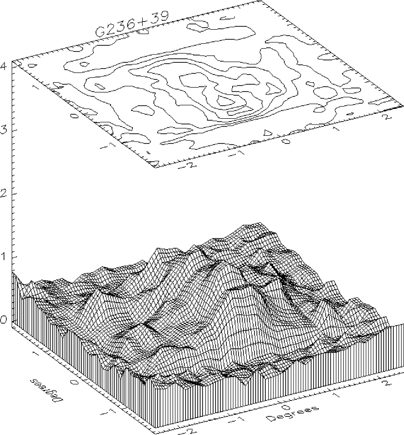
Figure 6:

Figure 1: Appendix

Figure 2: Appendix

Figure 3: Appendix

Figure 4: Appendix

Color Plate 1 may be viewed on the World Wide Web at URL:

http://www.pha.jhu.edu/\̃thinspaceneufeld/spaans+neufeld/plate1.html

Color Plate 2 may be viewed on the World Wide Web at URL:

http://www.pha.jhu.edu/\̃thinspaceneufeld/spaans+neufeld/plate2.html

The Web browser’s window should be set as large as possible to view these large color images.

References

- (1) Allison, A.C., & Dalgarno, A. 1970, Atomic Data, 1, 289
- (2) Black, J.H., & Dalgarno, A. 1977, ApJS, 34, 405
- (3) Black, J.H., & van Dishoeck, E.F. 1987, ApJ, 322, 412
- (4) Boulanger, F., & Pérault, M. 1988, ApJ, 330, 964
- (5) Crawford, I.A., & Barlow, M.J. 1996, MNRAS, 280, 863
- (6) Draine, B.T. 1978, ApJS, 36, 595
- (7) Jura, M. 1974, ApJ, 191, 375
- (8) Neufeld, D.A., & Spaans, M. 1996, ApJ, in press.
- (9) Reach, W.T., Koo, B.-C., & Heiles, C. 1994, ApJ, 429, 672
- (10) Roberge W.G. 1983, ApJ, 275, 292
- (11) Roberge, W.G., Jones, D., Lepp, S., & Dalgarno, A. 1991, ApJS 77, 287
- (12) Savage, B.D., Bohlin, R.C., Drake, J.F., & Budich, W. 1977, ApJ, 216 291
- (13) Spaans, M. 1996, A&A, 307, 271
- (14) Spitzer, L., Drake, J.F., Jenkins, E.B., Morton, D.C., Rogerson, J.B., & York, D.G. 1973, ApJL, 181, L116
- (15) Stephens, T.L., & Dalgarno, A. 1972, J. Quant. Spectroscop. Rad. Transf., 12, 569
- (16) Tielens, A.G.G.M., & Hollenbach, D.A. 1985, ApJ, 291, 722
- (17) van Dishoeck, E.F., & Black, J.H. 1986, ApJS, 62, 109
- (18) van Dishoeck, E.F., & Black, J.H. 1989, ApJ, 340, 273