Unifying models for X–ray selected and Radio selected BL Lac Objects
Abstract
We discuss alternative interpretations of the differences in the Spectral Energy Distributions (SEDs) of BL Lacs found in complete Radio or X–ray surveys.
A large body of observations in different bands suggests that the SEDs of BL Lac objects appearing in X–ray surveys differ from those appearing in radio surveys mainly in having a (synchrotron) spectral cut–off (or break) at much higher frequency.
In order to explain the different properties of radio and X-ray selected BL Lacs Giommi and Padovani proposed a model based on a common radio luminosity function. At each radio luminosity, objects with high frequency spectral cut-offs are assumed to be a minority. Nevertheless they dominate the X-ray selected population due to the larger X–ray–to–radio–flux ratio. An alternative model explored here (reminiscent of the orientation models previously proposed) is that the X-ray luminosity function is “primary” and that at each X-ray luminosity a minority of objects has larger radio–to–X–ray flux ratio.
The predictions of the two scenarios, computed via a Montecarlo technique, are compared with the observed properties of BL Lacs in the two samples extracted respectively from the 1 Jy radio survey and the Einstein Slew Survey. We show that both models can explain a number but not all the observed features.
We then propose a completely new approach, based on the idea that the physical parameter which governs the shape of the SEDs, is (or is associated with) the bolometric luminosity. Assuming an empirical relation between spectral shape and luminosity we show that the observational properties of the two surveys can be reproduced at least with the same accuracy as the two previous models.
keywords:
galaxies: jets, luminosity function – BL Lacertae objects: general – radiative mechanisms: non–thermal – surveys – methods: statistical1 Introduction
Among Active Galactic Nuclei, Blazars show extreme luminosity and variability. The observed properties are best interpreted in the frame of the relativistic jet model, proposed almost twenty years ago by Blandford & Rees (1978), as due to relativistic “beaming”, i.e. the effects of the relativistic motion of the emitting plasma on the observed radiation. In particular BL Lac objects, which are considered part of this class, are characterized by their almost featureless continua.
BL Lacs have been almost exclusively discovered through radio or X–ray surveys. However the properties of objects selected in the two spectral bands are systematically different, posing a question as to whether there are two “types” of BL Lacs. The first difference to be recognized and perhaps still the most striking is the shape of the SED. The differences show up using broad band spectral indices and color–color diagrams, e.g. vs 111; radio fluxes are taken at 5 GHz, optical at 5500 Å, X–ray at 1 keV (Stocke et al. 1985; Maraschi et al. 1995; Sambruna, Maraschi & Urry 1996). Others include optical polarization, variability, presence of (weak) emission lines, radio luminosity, core–dominance, all of which are less conspicuous in X-ray selected objects (e.g. Kollgaard et al. 1992; Perlman & Stocke 1993; Jannuzi et al. 1994; Kollgaard et al. 1996; see Kollgaard 1994 for a recent review).
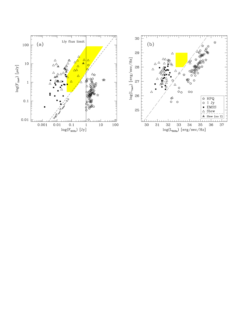
On the basis of the X-ray to radio flux ratio (or value) we can define an objective criterion (independent of the selection band) separating two (putative) classes of objects: we define XBLs the objects with and RBLs the objects with a ratio smaller than this dividing value, where the fluxes are monochromatic and expressed in the same units (see also Wurtz 1994, Giommi & Padovani 1994, for an analogous definition). As can be seen from Fig. 1a XBLs are found mostly but not exclusively in X-ray surveys and the same is true for RBLs with respect to radio surveys.
The spread in spectral shapes was originally attributed to orientation effects, associated with different widths of the beaming cones of the radio and X-ray radiation emitted by a relativistic jet (Stocke et al. 1985; Maraschi et al. 1986; Celotti et al. 1993). The idea came from the observational evidence that BL Lacs discovered in radio and X–ray surveys actually show similar X–ray luminosities while the radio luminosities typically differ by two–three orders of magnitude (e.g. Fig. 1b). This could be accounted for if X–ray radiation had a wider beaming cone than radio emission: observers would see similar X–ray luminosities over a wide range of angles while the accompanying radio luminosity would be high for a small fraction of objects seen at very small angles and strongly dimmed for the majority, observed at larger angles (e.g. Fig. 5 in Celotti et al. 1993). Consequently the number density ratio between the two “flavours” would be determined by the associated solid angles. Since the X–ray emission is largely isotropic, X–ray surveys are not biased against any of the two classes of objects, and can give the correct number ratio. The different beaming affecting the various bands could be due to an accelerating (Ghisellini & Maraschi 1989) or an increasingly collimated jet (Celotti et al. 1993).
Substantial progress in the data on the SEDs of BL Lac objects has been obtained in recent years, in terms both of sensitivity and statistics, especially in the X-ray band (Giommi, Ansari & Micol 1995; Comastri, Molendi & Ghisellini 1995; Perlman et al. 1996a,b; Urry et al. 1996; Sambruna et al. 1996). In terms of the power emitted per decade XBLs display a continuous rise up to the UV and in extreme cases the soft X-ray band, while RBLs are characterized by a spectral turn over in the IR domain. In XBLs the X-ray emission is dominated by a soft spectral component which extrapolates continuously to lower frequencies. In RBLs the X–ray emission is dominated by a separate harder component which at least in some cases extends to the –ray domain (von Montigny et al. 1995; for X–ray spectra see the results by Padovani & Giommi (1996) and Lamer, Brunner & Staubert 1996). A hard GeV to TeV component is present also in XBLs though it does not show up in medium energy X-rays. Sambruna et al. (1996) showed that it is difficult to model the detailed transition from an XBL to an RBL like in terms of orientation only and suggested rather a continuous change in the physical parameters of the jet.
The first model developed along this line to explain the “statistics” of XBLs and RBLs is the “radio luminosity + different energy cutoff” scenario by Giommi and Padovani (Giommi & Padovani, 1994; Padovani & Giommi 1995; hereafter we refer to it as the “radio leading” scenario by G&P) alternative in many ways to the commonly accepted “different viewing angle” model sketched above. They propose that a single luminosity function in the radio band describes the full BL Lac population. For each radio luminosity X–ray bright BL Lacs (i.e. XBLs) are intrinsically a minority described by a fixed (luminosity independent) distribution of X–ray to radio flux ratios222We note that the definition of XBL and RBL by G&P is based on the X–ray flux in the 0.33.5 keV Einstein IPC band (in erg/cm2/sec) and the radio flux at 5 GHz (in Jy). According to this different definition, the value of 5.5 adopted here corresponds to . In X–ray surveys however selection effects substantially enhance the XBL fraction. According to this approach the intrinsic fraction of the two types of BL Lac (XBL vs. RBL) would be objectively reflected in radio surveys. With these hypotheses G&P were able to reproduce the observed X–ray counts, luminosity functions and the distribution of BL Lacs in the plane.
Because of the implications of these issues for physical models of relativistic jets and the understanding of the physical conditions within the emission region, we decided to explore more thoroughly the fundamental hypothesis that BL Lacs are a single class, whose SEDs are characterized by different physical parameters, and test any prediction against the observations now available.
In addition to the radio leading model we consider a first “symmetric” alternative, namely that the X-ray luminosity function basically represents the whole BL Lac population. In this case X–ray surveys would give objective results regarding the intrinsic abundance of XBLs and RBLs. This scenario, which we refer to as the “X–ray leading” model, can be considered as an evolution of the “different viewing angle” scenario, where the X–ray luminosity was the basic property and the population ratio reflected the ratio of solid angles.
The predictions of both models, derived by a Montecarlo technique, are compared in detail with the observations now available. A main feature of the samples, that is the redshift distribution, appears poorly reproduced by either models.
We then propose a new, unified picture, in which the key feature is a link between the shape of the SEDs, in particular the peak frequency of the synchrotron power distribution, and the bolometric luminosity. In particular, we parameterize the shape of the SED in terms of its synchrotron peak frequency and assume a power law relation between peak frequency and bolometric luminosity. Adopting an estimate of the bolometric luminosity function we can derive all the observable properties and again compare them with observations.
We test all the scenarios against the best (whole) body of data now available: the radio and X–ray fluxes (uniformly measured by ROSAT, Urry et al. 1996) of the 1 Jy BL Lac sample (Stickel et al. 1991) and the radio and X–ray fluxes of the BL Lac sample derived from the Einstein Slew survey sample (Elvis et al. 1992; Perlman et al. 1996a). Based on the data and the discussion by Perlman et al., we treat the Slew survey sample available to date as a tentative, but quasi–complete one.
In Section 2 we present the radio and X–ray samples of BL Lacs against which we tested the predictions of the models. The two alternative “radio and X–ray leading” scenarios, as they will be called hereafter, are outlined in Section 3, while we describe the simulation procedure adopted for the comparison with the observed samples in Section 4. In Section 5 we present and compare the predictions of the two models with observations and briefly discuss the effects of evolution. The assumptions and predictions of the new “unified bolometric” model are described in Section 6. Section 7 summarizes our conclusions.
The values km/sec/Mpc and have been adopted throughout the paper.
2 The reference samples
2.1 The 1 Jy sample
The complete 1 Jy BL Lac sample was derived from the catalog of radio selected extragalactic sources with Jy (Kühr et al. 1981) with additional requirements on radio flatness (, with ), optical brightness () and the absence of optical emission lines (EW Å, evaluated in the source rest frame) (Stickel et al. 1991). This yielded 34 sources matching the criteria, 26 with a redshift determination and 4 with a lower limit on it (Stickel et al. 1994). It is the largest complete radio sample of BL Lacs compiled so far.
We computed the luminosities using the monochromatic 1 keV fluxes measured by ROSAT (Urry et al. 1996, where the listed values are those from fits with Galactic absorption) and the 5 GHz values from the Kühr et al. catalogue. We considered only the subsamples of sources with at least a lower limit on the redshift. The fluxes were K–corrected using a radio spectral index and the average X-ray spectral index measured in the ROSAT band, .
2.2 The Slew survey sample
The Einstein Slew survey (Elvis et al. 1992) was derived from data taken with the IPC in between pointed observations. A catalog of 809 objects has been assembled with a detection threshold fixed at 5 photons. It does not reach high sensitivity, having a flux limit of erg/cm2/sec in the IPC band (0.3 3.5 keV), but it covers a large fraction of the sky ( 36600 deg2). Based on radio imaging and spectroscopy Perlman et al. (1996a) selected from this sample a set of 62 BL Lac objects (33 previously known and 29 new candidates) and, in a restricted region of the sky, a quasi–complete sample of 48 BL Lacs. The sources are almost completely identified, and therefore constitute a quasi–complete sample of 48 BL Lacs. The redshift is known for 41 out of 48 objects. This is the largest available X–ray selected sample of BL Lacs (Perlman et al. 1996a), with more than twice the number of sources contained in the fairly rich X–ray selected sample derived from the Einstein Medium Sensitivity Survey (EMSS, Morris et al. 1991, Wolter et al. 1994; Perlman et al. 1996b), extended to 23 objects by Wolter et al. (1994).
K–corrections of the radio and X–ray monochromatic fluxes were computed using spectral indices and , respectively.
3 The two scenarios
3.1 Different energy cut–off
Giommi and Padovani introduced the idea that BL Lacs are a single population of objects whose SED can be characterized phenomenologically by the distribution of the values of the frequency at which the peak in the energy emitted per logarithmic bandwidth occurs (i.e. the peak in the representation of the broad band energy distribution) for the putative synchrotron component.
A good quantitative indicator of the overall broad band shape of SEDs is the ratio between X–ray and radio fluxes, conventionally taken at 1 keV and 5 GHz, equivalent to a characterization in terms of and (for a representation of the relation between SED shape and for instance see Fig. 2 in Maraschi et al. 1995; Comastri et al. 1995 tested also the correlation). SEDs peaking at lower frequencies correspond to higher ratios (e.g. Maraschi et al. 1995). The X–ray to radio flux ratio is typically two orders of magnitude larger in BL Lac objects derived from X–ray surveys than in objects derived from radio surveys.
It is clearly more convenient to work with flux ratios since they are easier to determine then the peak frequency of a broad band energy distribution. One can even observationally derive a distribution for the X–ray/radio luminosity ratio as if this is the relevant intrinsic quantity which characterizes the SED distribution. This is what we consider hereafter, following the G&P approach.
Starting from these hypothesis, one can derive the statistical properties of BL Lacs simply by assuming a radio (X–ray) luminosity function and a probability distribution, , of the X–ray to radio luminosity ratio. In the following two subsections we present the assumptions on these two quantities, according to the radio leading model and its symmetric, in which the X–ray luminosity is the leading one.
3.2 “Radio luminosity leading”
The basic radio leading (G&P) hypothesis (Giommi & Padovani 1994; Padovani & Giommi 1995) is that radio selection would be objective with respect to the intrinsic spread of broad band spectral properties. The underlying idea is that the radio emission is only weakly affected by the properties of the synchrotron component at higher energies, such as the peak frequency. Therefore the radio selection is not expected to suffer of any bias regarding the SED shape properties and sources with different X–ray/radio luminosity ratios are sampled from a common radio luminosity function.
In this approach, the X–ray counts (and X–ray luminosity function) are easily predictable from the radio counts (and radio luminosity function) and the results can be compared with real data coming from surveys. It is worth reminding that there are essentially no free parameters in the model.
Since a radio selected sample would be unbiased with respect to the X–ray to radio luminosity ratio, G&P considered the 1 Jy sample of BL Lacs (Stickel et al. 1991) and built the probability distribution . To improve the statistics for the XBL–like objects part of , we considered, following Padovani and Giommi (1995), the distribution deduced from the EMSS sample, weighted by a factor 1/10. In fact the ratio of XBL to RBL objects derived from various radio selected samples (1 Jy, Stickel et al. 1991; S4, Stickel & Kühr 1994; S5, Stickel & Kühr 1996) covers the range 1/16 1/6. Therefore, with the given hypothesis, this factor 1/10 represents the intrinsic ratio of XBL to RBL populations in the whole BL Lac class: in the radio leading scenario only a minority of sources would intrinsically have the SED peaking in the UV range, while most of the energy distributions would peak in the IR range.
To calculate the luminosity function in the luminosity range [erg/sec/Hz], G&P extrapolated the observed one to lower luminosities. This extrapolation is based on the beaming model scheme (see Urry et al. 1991), applied to the luminosity function derived from the 1 Jy sample data (covering the range erg/sec/Hz, Stickel et al. 1991), in the non evolutionary case. We note that the predictions of the model are indeed strongly dependent on the number density of the low luminosity sources.
Clearly, the assumption of a minimum radio luminosity introduces a limiting luminosity in the X–ray band, . However, it is worth noting that, because of the different spectral shape of XBL and RBL objects, their corresponding minimum luminosities will be different, with .
G&P found a good agreement between the predicted X–ray counts and those derived from all the main X–ray surveys (EMSS, EXOSAT High Galactic Latitude Survey, HEAO-1 surveys; see Fig. 3 of Padovani & Giommi 1995) and with the EMSS luminosity function.
In their model, the observational evidence that XBL objects are more numerous, apparently in contradiction with their assumption that XBL sources are intrinsically only 1/10 of the entire population, is due to selection effects. In fact, given their ratios, XBL have a relatively low radio flux. Therefore, at the same X–ray flux level we are detecting together BL Lacs belonging to different parts of the radio luminosity function, with RBLs coming from a brighter but poorer part of it.
Our aim here is to perform a further step in checking the radio leading scenario, i.e. to compute the distribution of radio and X–ray luminosities predicted for samples selected in the “leading” (radio) band also in the “secondary” (X–ray) spectral band, using the same inputs of G&P.
3.3 “X–ray luminosity leading”
The first alternative scenario that we tested is substantially “symmetric” to the radio leading one. It assumes that the common property of XBL and RBL is the X–ray luminosity. As already mentioned, this idea originally comes from the observational evidence that BL Lacs discovered in radio and X–ray surveys actually show similar X–ray luminosities, while the radio luminosities typically differ by two–three orders of magnitude (e.g. Maraschi et al. 1986; see also Fig. 1b). This is in general true also if the distinction between the two types of sources is made in terms of the RBL/XBL classification as formally defined in Section 1 (see also Fig. 1a).
Again, the starting points are the X–ray luminosity function and a probability distribution, , of luminosity ratios, but in this case this should be observationally derived from an X–ray survey, that by construction is now supposed to be the objective one.
An important assumption, which we had necessarily to take into account in the X–ray case, concerns the cosmological evolution of BL Lacs. While it has been so far established that RBLs show a slight positive evolution, consistent with no evolution at the 2 level (e.g. Stickel et al. 1991; Wolter et al. 1994), recently Wolter et al. (1994) and Perlman et al. (1996b) confirmed the strong negative evolution in the X–ray band: X–ray bright objects are much less luminous or common at high redshifts. In analogy with the radio case, we first evaluated the predictions of the X–ray leading model assuming no evolution. The results have been presented by Fossati et al. (1996) who showed that they are not compatible with the 1 Jy survey properties, predicting a number of RBL objects in large excess with respect to the observed one.
Then, in order to be able to reproduce the observational results and in particular the redshift distributions (see below), here we assumed a negative luminosity evolution in the X–ray band.
We derived the distribution from the Slew survey X–ray selected sample, but using only objects with redshift lower than 0.25, in order to better approximate a distribution appropriate for a sample of sources at the same redshift.
Unfortunately, the X–ray luminosity function for this sample is not (yet) available. For this reason we considered the EMSS and its well studied X–ray luminosity function (Morris et al. 1991; Wolter et al. 1994). We tentatively adopted an X–ray luminosity function matching that derived by Wolter et al. (1994), represented as a single power law with slope = 1.62. Since the normalization of the luminosity function would substantially affect only the total number of sources, but neither their relative number nor the average luminosities, in order to recover the correct absolute number of objects we fixed the normalization (for the case with best results reported in Table 1) at the value . This value is within the confidence range given by Wolter et al. (1994), with corresponding to erg/sec.
The luminosity evolution parameter is = 0.142, according to the definition , where is the look–back time in units of t0 (for , t0 = 1/H0). The luminosity range is [erg/sec/Hz]. Also in this case we stress that RBLs and XBL reach different values of the minimum radio luminosity (see Section 3.2).
4 The simulations
Given these assumptions, we computed the predictions of both models. We used a Montecarlo technique to simulate the distribution of sources in space and luminosity. This method is very convenient because it allows us to store “single source” attributes and not only to compute sample integrated average properties. In other words, we can actually simulate a catalogue and from it compute the desired average quantities.
For the “radio leading” scenario we used a third degree polynomial fit to the luminosity function published in Fig. 1 of Padovani & Giommi (1995)333The polynomial fit is expressed as Gpc-3 L-1, where erg/s/Hz, and , , and . In all cases simulations have been performed within the redshift range .
In Fig. 2a,b the observed distributions are shown, taking into account only objects with redshift estimate. The dashed histograms represent RBL objects, the dotted ones XBLs. Note that there is a superposition of the two classes due the fact that the actual distinction between RBL and XBL is based on the flux ratio (while here the luminosities are considered). In Fig. 2c the distribution , used in the calculations for the radio leading scenario, is shown.
The actual computation can be summarized in five steps:
-
1.
“draw” a redshift and a luminosity from the luminosity function assumed as primary (radio for the radio leading, X–ray for the X–ray leading scenarios);
-
2.
the “secondary” luminosity (i.e. in the other spectral band) is deduced by choosing a luminosity ratio by means of its probability distribution ;
-
3.
radio and X–ray fluxes are computed for the simulated source taking into account the “inverse” K–correction444The “inverse” refers to the fact that usually the K–correction is meant to convert observer–frame to source–frame quantities, while here we are using it in the other direction.;
-
4.
check if the simulated source would be detected in a survey with a given flux limit and, if so, store its set of parameters.
The detectability criteria take into account the sky coverage that in the radio case is a step function of the monochromatic 5 GHz flux, while in the X–ray survey it is an increasing function of the flux integrated over the whole IPC band (0.3 3.5 keV). In the X–ray case we then simulated N surveys (typically 15 20) each with a different flux limit and a corresponding . The results of the N surveys are then summed up to construct the full X–ray survey.
The flux dependent sky coverage for the Slew survey has been derived from the diagram “exposure time” vs. “percentage of sky” published in Elvis et al. (1992). A limiting flux corresponding to a given exposure time is deduced considering a detection limit of 5 IPC counts, and a conversion factor from IPC counts to flux of erg/cm2/sec (Elvis et al. 1992), valid for values of and cm-2. In fact, in order to convert to monochromatic flux we adopted an X–ray spectral index , a fiducial average value for the class of sources that we are considering. This gives the conversion relation: . It is important to stress here that we use an approximated sky coverage by using the information currently available. An exact correction cannot be computed, but plausibly this would mostly affect the normalization of the assumed luminosity functions.
-
5.
finally, a detected source is classified as XBL or RBL according to its ratio, as already defined.
5 Results and comparison of the models
The comparison of the two models with the 1 Jy and Slew survey samples are presented in Figs. 3 and 4, respectively. The average observed and predicted radio and X-ray luminosities are reported in Table 1, together with the numbers of objects. The consistency of the predicted and observed distributions has been quantitatively estimated through the use of the Student’s t–test for comparison of the means, and also of the more sophisticated survival analysis non-parametric and univariate methods (Feigelson & Nelson 1985) allowing to take into account lower limits. Student’s t–test has been performed on all average luminosities, while the survival analysis has been applied only to the cases with a significant number of objects, namely for the RBLs subsample in the “1 Jy” and XBLs in the Slew survey. The results of the statistical tests are reported as an entry in Table 1 for Student’s t–test, and separately in Table 2 for the survival analysis.
Radio survey
Let us consider first the comparison of the models with the 1 Jy sample (Fig. 3).
Both models predict luminosities for the XBL in both bands more than one order of magnitude larger than observed. However the extreme paucity of objects does not allow these discrepancies to be significant from a statistical point of view. The Student’s t–test indicates that the radio leading scenario predicts a disagreement, at the 94.0 per cent level, in the X–ray luminosity of the RBL, while the X–ray leading one has difficulties at reproducing the average luminosity of the XBL at the 91 per cent level.
The relative number of objects detected in both scenarios is in reasonably good agreement with the observed one (5/29 and 3/27 instead of 2/32).
X–ray survey
The predictions of the two models concerning the Slew survey objects are instead quite different (Fig. 4).
The radio leading scheme leads to incorrect X–ray and radio luminosities of XBL: from survival analysis 97.2 and 99.96 per cent levels (Table 2), respectively, even worst according to the Student’s t–test (Table 1). In particular, in the radio leading scenario the average radio luminosities of the RBL and XBL subsamples tends unavoidably to be the same: as immediate consequence of the “radio leading” hypothesis, all BL Lac objects should share the same range of radio luminosity, in contrast with observations of complete samples (see also Fig. 1b). The average radio luminosity of XBL is also overestimated within the X–ray leading scenario ( per cent level). Again, nothing can be said from these tests on the distributions of the less numerous source population.
The predicted numbers of XBLs and RBLs in the Slew survey (43/7 and 43/7) are in good agreement with the observed one (40/8).
Summarizing, in terms of source numbers and average luminosities the X–ray leading model is better than the radio leading one, sharing with it the problem of XBL luminosities in radio surveys. Nevertheless, it should be noted that XBL objects in the 1 Jy survey are only 2 and so their measured properties could mis–represent the true ones.
Redshift distribution
Finally, there is a significant disagreement on the red-shift distributions (see the panels of the first columns in Figs. 3 and 4): both models predict a sharp peak of simulated RBL sources at low redshift, in contrast with the observed flat distributions555Note that the inconsistency between the distribution predicted by the radio leading scenario and the one observed in the 1 Jy sample is in agreement with the assumption of no evolution adopted here. If we had introduced the slight positive evolution apparent from “1 Jy” data we would have obtained a redshift distribution completely consistent with the observed one..
This is a built–in feature of this kind of approach in which we take the relative number of the the two types of sources fixed for any value of the leading luminosity.
Note however that, as expected, the inclusion of the negative evolution in the X–ray leading model tends to improve the agreement with observations. Indeed the redshift distributions obtained in the X–ray leading non evolving case were qualitatively similar to the ones of the radio leading scenario (see Fossati et al. 1996). In fact in the 1 Jy survey XBLs are sharply concentrated at lower redshifts, while RBLs show a “flatter” distribution. These trends are closer to the observed ones than those derived in the radio leading scenario (Fig. 3). The same is true for the Slew survey (Fig. 4).
The use of the survival analysis allowed us to perform a quantitative analysis. The comparison of the only RBLs in the 1 Jy survey indicates that the predicted distributions are not compatible with the observed one at the 95.80 and 93.45 per cent level for the radio and X–ray leading scenarios, respectively. A much more significant disagreement is found in the Slew survey (considering only XBLs), which is inconsistent with the predictions of the radio leading scenario at the 99.96 per cent level.
5.1 Evolution
This last point on the redshift distribution is particularly important. In fact it indicates that evolutionary effects should be taken into account. However it is possible that it is the distribution which changes with redshift, rather than the luminosity in one of the two bands: clearly one can re–express the different evolution in the two bands, by saying that evolves.
From an observational point of view, if one considers different intervals in redshifts in the Slew survey sample there are 5 RBL and 7 XBL objects at high redshifts, while these numbers become 3 and 26 at low redshifts (taking a dividing value at ). The only two XBL sources with known redshift present in the 1 Jy sample are both at .
We then considered an evolving probability distribution , i.e. we introduced a redshift dependence on the relative ratio of the two populations of BL Lac objects. Basically has a bimodal shape, described with two gaussians centered at and 3.5 for RBLs and XBLs, respectively. The relative normalization of these gaussians evolves as (with ), in such a way that the RBL part of the distribution becomes more and more dominant at higher redshifts. With this evolution of we can induce the observed difference in the redshift distribution of XBLs and RBLs.
In this case the luminosity function is not self–consistently derived. Instead, we have to deal with a tentative luminosity function, in the sense that it is by no means consistent with the evolution that we are introducing. It is therefore necessary to derive “backwards” how the evolution of translates in terms of luminosity function evolution.
We considered only a limited region of the parameter space of and , without finding a solution which improves the results already obtained. Actually, in the case of the radio leading scenario, there is a hint that better solutions are obtained by changing the parameters progressively towards the no evolution case, as in the G&P model.
While we cannot exclude that a suitable solution could be found following these assumptions, we decided to consider a new approach “a priori”, described in the following section.
6 Unified bolometric approach
6.1 The idea
Partly motivated by the difficulties found with the models discussed so far, we tried a completely different way of facing the problem. Furthermore, we wanted to take into account the properties of the overall observed SED of BL Lacs, as well as recent indication of a possible link, along a continuous sequence, between the SED shape and the source luminosity (e.g. Sambruna et al. 1996, Ghisellini et al., in preparation).
The fundamental hypothesis of the model is still that XBL and RBL sources are manifestations of the same physical phænomenon. The new ingredient is the idea that XBLs and RBLs are different representatives of a spectral sequence that can be described in terms of a single parameter, which we identify with the bolometric luminosity of the synchrotron component, . Both “flavours” of BL Lac objects share the same bolometric luminosity function and the SED properties depend strongly on this quantity.
The main positive feature of this approach is that it offers a more direct interpretation in terms of the physical properties of these sources. In fact:
- a)
-
the assumptions are largely independent of the details of the observed statistical samples and moreover they are not based on the choice of a leading spectral band;
- b)
-
there is an immediate connection between the parameters of solutions “acceptable” from a statistical point of view and the physical conditions of the emitting plasma (see Section 7).
The relation between the bolometric luminosity and the SED has been based on observed trends. More luminous objects seem to have RBL–type spectral properties, with the peak of the energy distribution in the IR–optical range and Compton dominated soft X–ray spectra.
The less luminous sources tend to display XBL–like SEDs, steep soft X–ray spectra and a synchrotron component peaking in the UV–soft X–ray band (e.g. Fig. 1b). The distribution between this two extremes seems to be continuous and we propose that it is governed by the now leading parameter . Therefore, if we characterize the SED with the frequency at which the (synchrotron) energy distribution has a maximum, a fundamental (inverse) relation must exist between the bolometric luminosity and this frequency. The inverse dependence is qualitatively based on the trend found by Ghisellini et al. (in preparation).
Interestingly, note that the different redshift distributions of the two kinds of BL Lacs could be a natural outcome of this scenario. XBLs objects come from the lower (and richer) part of the luminosity function and so they would dominate at low redshift, but they would disappear at large distances despite the increase of the available volume. On the contrary, RBLs, even though coming from the poorer part of the luminosity function, would become predominant at higher redshifts, being still detectable.
In the next Sections we discuss a parameterization of the observed SEDs, which allows us to quantify the predictions of this model.
6.2 SEDs parameterization
In order to reproduce the basic features of the observed SEDs we considered a simple two component model. The synchrotron radio to soft X–ray component is represented with a power law in the radio domain, with spectral index , smoothly connecting, at , with a parabolic branch ranging up to . Beyond the synchrotron component steepens parabolically.
The hard X–ray Compton component is simply represented with a single power law with spectral index . The normalization at 1 keV of this hard component () is kept fixed relative to the synchrotron one at 5 GHz (). This immediately implies a correlation between the radio and X–ray luminosity in sources where the emission at 1 keV is dominated by the Compton emission.
The parameters describing this representation of the SED are then five: , , the hard (Compton) X–ray normalization K, and either the width of the parabolic branch or . This is because we require that the parabolic branch matches the flat radio component at also in its first derivative, and therefore we cannot fix independently both its width and peak frequency. A schematic representation of this parameterization is shown in Fig. 5, while its analytical expression is reported in Appendix A.
For simplicity, we use the luminosity at the peak of the synchrotron component, instead of the bolometric luminosity. In fact, for various complete samples of BL Lacs, Sambruna et al. (1996) find that the ratio between and is consistent with being constant, .
We then specify the relation between (the frequency at which the peak in the representation occurs) and the value of ( is the flux in the source frame). This is the key physical relation of the proposed model. For simplicity we considered a simple power law dependence ()666We note that hereafter indicates the equivalent of a bolometric luminosity, i.e. evaluated at .. We then have three more parameters: , and .
In Fig. 6 a set of SEDs following the adopted parameterization is shown. The dashed lines represent those with , roughly corresponding to XBL–type objects, while the opposite is true for the solid ones, RBL–type objects. Remember that the distinction is actually defined in terms of the flux ratio, and that .
To summarize: the adopted parameterization requires 8 inputs, 5 describing the shape of the SED (, , , , ) and three its relation with the luminosity (, , ). However, the family of SEDs is completely determined by a set of 7 parameters, because the first 5 reduce to 4 1, (, , , , ). In addition we must specify the normalization and the slope of the adopted luminosity function.
6.3 SEDs: parameterization vs observations
Despite the number of parameters, there is only a limited freedom in the choice of their values, which are constrained by observations.
-
only takes values in a narrow range around 0, and we perform our simulations with the fiducial values 0.0, 0.1, 0.2.
-
The value of is constrained by the assumption that, in the case of extremely hard X–ray spectra, we are only looking at the Compton component. We then considered a single value of equal to the slope of the flatter X–ray spectra of RBL (Lamer et al. 1996, Urry et al. 1996), for which we can think that we are measuring only their Compton emission.
-
On the same basis, the relative normalization between the radio and the X–ray components can be constrained by the value of of extreme RBL type objects, i.e. in the range [8 ; 7]. We adopted the values and .
-
can be limited by the ranges of observed and , which imply values of between 1 and 2.
-
is the parameter less determined by observations, being difficult to identify a spectral break even in the case of the best sampled and simultaneous SED. We considered values between and Hz. In the context of this parameterization the actual importance of is indirect: its position affects the width of the parabolic branch extending up to the X–ray band. For a fixed value of the higher is , the narrower will be the parabola (i.e. the steeper the cut–off).
Let us consider now some observed properties of complete BL Lac samples, which allow us to check the goodness of our parametric representation.
In Fig. 7, the classic vs plane for BL Lacs is shown, with points representative of the 1 Jy, Slew and EMSS samples. The line crossing the diagram is the locus of points derived from our “best fit” SEDs. It basically reproduces the observed pattern of two different branches, where RBLs and XBLs are concentrated, apparently with no overlapping. The fact that the “synthetic path” does not extend beyond is related with the narrow range of parameters (and tight relation among them) adopted in the samples simulation, namely to the minimum allowed bolometric luminosity.
It is also possible to compare the SEDs with the observed average spectral energy distributions of RBLs and XBLs, taken from Sambruna et al. (1996). Their data points, given in flux units and converted in luminosities (considering a typical redshift of 0.5 for the RBLs and 0.2 for XBLs), are plotted in Fig. 6 together with our SED family. Also in this case the agreement is satisfactory.
Finally, also the vs diagram (see Fig. 1b) can be interpreted in terms of the SEDs of RBLs and XBLs. There is a fixed relation connecting the synchrotron radio luminosity and the inverse Compton X–ray luminosity and this can be better observed in RBLs, where more likely the Compton component dominates the X–ray emission. RBLs then occupy a locus following this correlation. The XBLs on the contrary lie away from this line because their X–ray emission is progressively dominated by a different component, the extreme part of the synchrotron spectrum.
We indeed verified that the luminosity correlation for RBL seen in Fig. 1b is not purely due to the common dependence on redshift of and . A Kendall’s test gives a correlation at 99.99 per cent level, which is still present, even though at the 96.8 per cent level, when the redshift dependence is excluded. Furthermore, we tried to establish the real nature of the lack of observed sources in the region around =33 and =28.5. The results are shown in Fig. 1a, which is the equivalent plot, where fluxes (and not luminosities) are considered. The vertical and oblique lines represent the flux limit of the 1 Jy survey and the ratio of the fluxes defining XBL and RBL (i.e. 5.5), respectively. The grey area of the diagram shows the position in this flux–flux plane of putative sources with luminosities in the empty area of Fig. 1b (indicated with similar shading) when we imagine to move them in distance, covering a range of redshift between . It can be seen that there is no apparent observational bias against detection of sources with those luminosities: this indeed suggests that the lack of objects is plausibly linked to their intrinsic properties. This fact seems therefore to qualitatively agree with the shape of the SED assumed in the bolometric scenario.
Clearly, none of the above checks concerns the number density of objects. We adopted a luminosity function for inspired to that calculated by Urry & Padovani (1995) (see their Fig. 13) for the 1 Jy and EMSS BL Lacs. Their (bivariate) luminosity function is obviously affected by selection effects both in the X–ray and radio bands, but constitutes the available distribution closest to a truly ‘bolometric’ one. The normalization has been chosen in the range to 44.5 and the index to 2.3: also on these parameters we have a limited freedom. Note that the normalization is not actually an interesting parameter and, as already mentioned in Section 3.3, varying only affects the absolute number of sources, neither the relative number of the two kinds nor the average luminosities. Finally, we stress that for simplicity no evolution has been assumed in the bolometric scenario.
To conclude this Section, we can say that our schematic representation of the SEDs well reproduces the basic properties of the observed BL Lacs broad band spectra. We have 9 parameters and 14 observational quantities to match (8 average luminosities and 6 source numbers).
6.4 Results
Even a simple “first attempt” set of the 9 input parameters gives a surprisingly good output. In Table 1 the best results, found after a systematic check for a grid of parameter values within the allowed ranges, are reported. The corresponding input parameters are listed in the note to the Table.
The Student’s t–test implies that the model predicts too high luminosities for the RBL both in the radio and X–ray band (at the 99.9 and 98.6 per cent level, respectively, see Table 1) when compared with the observed 1 Jy Survey distributions. The result is confirmed by the survival analysis (see Table 2). For the Slew survey instead no significant disagreement has been found.
Furthermore, a very positive consequence of this scenario is that it implies a qualitatively ‘better’ redshift distribution, as can be seen in Figs. 3 and 4, with respect to the previous schemes. In particular we stress that the bolometric scenario is the only one which predicts, as direct result of the SED dependence on the bolometric luminosity, that the redshift distributions of the two populations can be such that RBL would tend to dominate at high redshifts, while the opposite would be true at low (see Fig. 4). This behaviour could be seen as equivalent to either a redshift dependence of the X–ray-to-radio–flux ratio distribution or a negative X–ray luminosity evolution.
There is still a problem with RBLs in the radio survey. Even though the shape of the distribution is correctly flat (and this is the major difficulty of the two other models), it extends well beyond , which leads to a disagreement significant at the 92.7 per cent level (survival analysis). We believe this fact is directly connected with the excessive average radio luminosities predicted by the model.
In order to explore the consistency of the shape of the predicted and observed redshift distributions, we applied the survival analysis test only up to , and did not find inconsistency between the two. with the observed one. Clearly, this result only indicates that the shape of the predicted distribution can resemble the real one over the considered redshift interval. However, as we discuss in Section 7, the excess of objects predicted at higher redshift (and/or their overestimated radio power) could be understood in an even broader unifying picture.
7 Discussion and conclusions
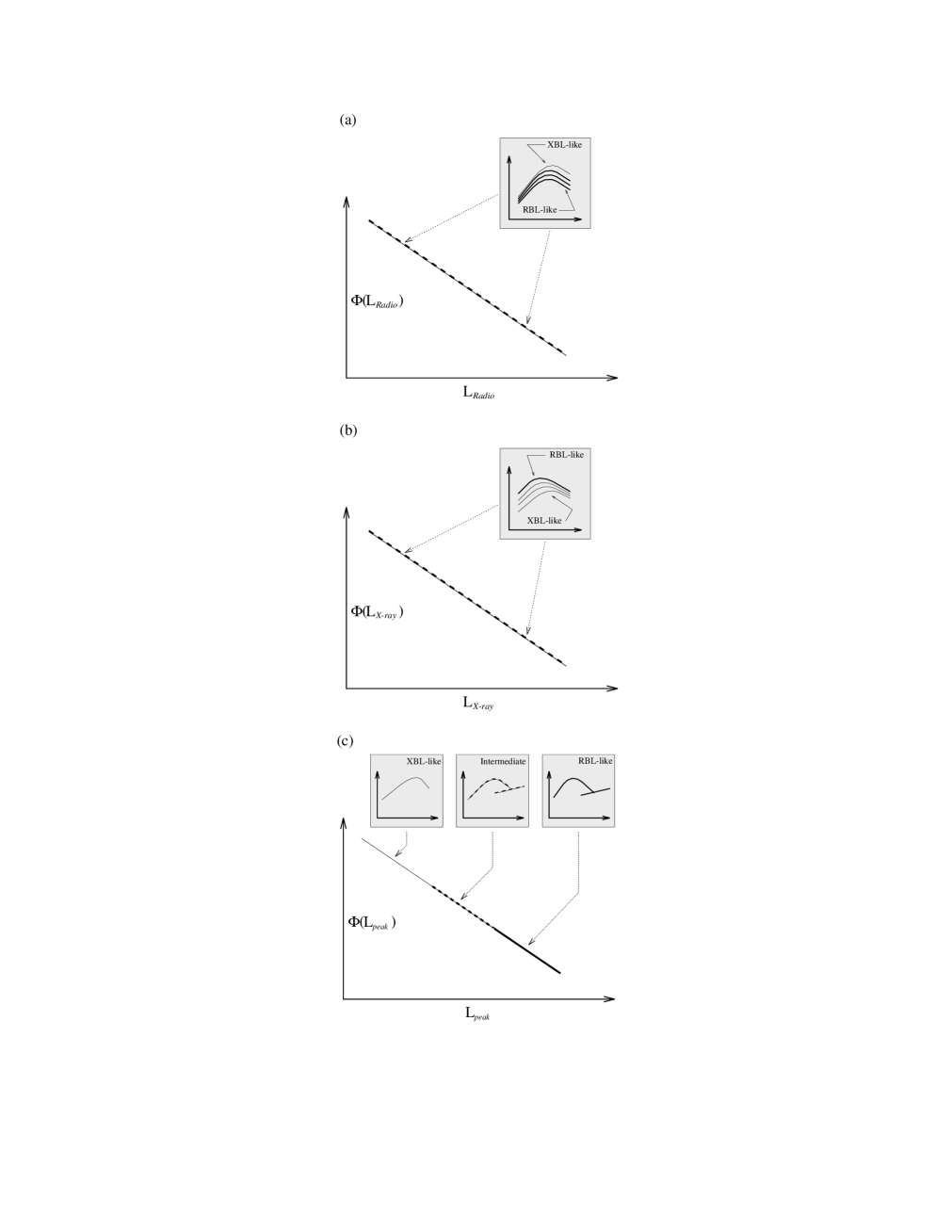
We have considered three different scenarios, which assume that BL Lac objects constitute a single population of sources, with different spectral energy distributions (mainly different peak frequencies of the synchrotron component), which originally mislead into thinking of a separation of BL Lacs into two classes.
A representation of the main features of these scenarios is shown in the cartoons of Fig. 8a,b,c.
Two of these models (namely the radio and X–ray leading ones; see Fig. 8a,b) are symmetric, and differ in the choice of the leading parameter, i.e. the radio and X–ray luminosities, respectively. The models are constructed from observed properties, like the luminosity functions and the probability distribution of the flux ratios, with basically no free parameters. They can correctly predict a significant number of quantities in agreement with current observations. However they (and in particular the radio leading one) fail to reproduce some of the observed distributions.
We then proposed a unified bolometric model (see Fig. 8c), whose main characteristic is to link the bolometric luminosity with the energy of the synchrotron cut–off. This scenario is based too on observational trends, however it uses a schematic parameterization of the BL Lac SED as well as a semi–empirical luminosity function for the bolometric luminosities. We stress here that while it is true that the bolometric scenario contains a significant number of (quite constrained) parameters with respect to the two other models, it also predicts the statistical and cosmological properties of the two ‘types’ of sources directly from a unified description of their spectral distribution. And, despite the rigid formulation of the one–to–one correspondence between the SED properties and the luminosity, in this scenario the main observational data can be reproduced at least with the same ‘accuracy’ as the other two models. Particularly interesting is the prediction of the different XBL and RBL redshift distributions, which tend to favour the detection of objects of the first class at low redshifts and of RBL at higher .
The predictions of the bolometric model of luminosities of sources detected in radio surveys higher than observed is plausibly related to the problem with their redshift distribution. We note, in fact, that the inclusion of Highly Polarized Quasars (HPQ) (i.e. emission line Blazars) in the – and colour–colour distributions shows an interesting continuity of their properties with those of BL Lacs (see Figs. 1 and 7, where stars represent HPQ). In particular, the significance of the correlation between and (see Section 6.3) increases to 99.99 per cent (already excluding the common dependence on redshift) when also the HPQ of the Impey & Tapia (1990) sample are included. The morphology of the extended radio emission of some RBL (see e.g. Kollgaard et al. 1992; Perlman & Stocke 1993), and the radio luminosity functions of RBLs and FSRQ (a class of Blazars substantially equivalent to HPQ) also show continuity (Maraschi & Rovetti 1994). All these pieces of evidence lead to the suggestion that there is actually a remarkable progression in properties, in a luminosity sequence XBL–RBL–HPQ, which is also a sequence of increasing importance of emission lines. If a fraction of the sources with the highest bolometric luminosities could be indeed “classified” as HPQ rather than RBL (in a way analogous to the transition from XBLs to RBLs), this fact could plausibly explain the discrepancies in the high luminosities and redshift distributions predicted by the model.
As already stressed, a very interesting aspect of the “bolometric” approach is that it is based on the relative dependence of two quantities which are strongly related to the physical properties of the emitting plasma, namely the emitted luminosity and the cut–off in the synchrotron spectrum. One can therefore speculate on the physical origin of this dependence.
Probably the simplest interpretation of this link is that it is directly related to the particle cooling. The more radiation is emitted the more particles loose energy, with consequent decrease in the cut–off frequency (which reflects the maximum energy of the emitting particles). If the energy of the particles emitting at the peak of the flux distribution is determined by the escaping time from the emitting region, this can be estimated by equating the cooling and a typical escape timescales. This leads to the relation , where is the size of the emitting region. This dependence is reasonably close to the one which predicts the best results of the model (). Clearly this interpretation is not unique and one can as easily envisage physical scenarios where a different relation between these two quantities is expected (e.g. in the case the source size is proportional to the central object mass).
Furthermore the relation can be also attributed, in the context of inhomogeneous jet models, to a possible dependence of the length of the collimated jet on the radiated power: more powerful jets could extend farther and originate outer radio regions responsible for the X–ray Compton component.
To conclude, we consider here the predictions of the models examined on the results of deeper surveys. In particular we compute the expected ratio of objects of the two “flavours” in more sensitive radio and X–ray surveys, as a function of their flux limits. The results are reported in Table 3777Browne & Marchã (1993) pointed out the possible effect of misidentification of faint BL Lacs caused by the lack of contrast of the active nucleus with the host galaxy. It should be noted here that, while we were able to ignore the Browne & Marchã selection effect for the results of the Slew survey, this would be progressively relevant in surveys with decreasing flux limit, as the ones we are simulating here., as the relative ratio normalized to the value predicted for the 1 Jy and Slew surveys.
Note that this ratio is a function of the flux limit even in the radio survey for the radio leading scenario (and X–ray survey for the X–ray leading one). This is due to the different dominant range of redshifts at different flux limits, which causes objects at the border of the definition of XBL/RBL to “move” into the RBL class, because of the term (always 0) in the relation between flux and luminosity ratios.
Another factor to take into account in the interpretation of these predictions is the influence of the minimum luminosities. As mentioned in Section 3.2, a minimum luminosity in the “leading” band leads to different minimum luminosities for RBL and XBL in the “secondary” band, due to their intrinsically different SEDs. Therefore, at flux limits which allow the detection of the faintest sources, only objects with SEDs which favour very low fluxes in that band will be detected. This effect is observable mainly in radio surveys in the X–ray leading scenario and in X–ray surveys in the radio leading one.
From Table 3, one can clearly see the opposite trends expected from the radio and X–ray leading scenarios in radio surveys. Distinct features of the bolometric scenario are a rapid decline in the fraction of RBL in radio surveys and a weak decrease in X–ray surveys. This behaviour follows from the one–way relation between RBL and XBL SED properties with luminosity.
Acknowledgments
We thank F. Rovetti and A.Treves for their helpful collaboration in early stages of this work and the referee, Paolo Padovani, for his careful report and useful suggestions. GF and AC acknowledge the Italian MURST for financial support.
8 Appendix A: SED parameterization
The analytical expression of the parameterized SEDs in the “bolometric” model is given by:
where , and , and . and are defined on the frequency ranges and , respectively.
The SED expression can be re-scaled as a function of the value of , and in particular the luminosities at 5 GHz and 1 keV can then be written as:
References
Blandford R., Rees M.J., 1978, in Pittsburgh Conference on BL Lac Objects, ed. A. N. Wolfe (Pittsburgh:Pittsburgh Univ. Press), 328
Browne I.W.A., Marchã M.J.M., 1993, MNRAS, 261, 795
Brunner H., Lamer G., Worrall D.M., Staubert R., 1994, A&A, 287, 436
Celotti A., Maraschi L., Ghisellini G., Caccianiga A., Maccacaro T., 1993, ApJ, 416, 118
Comastri A., Molendi S., Ghisellini G., 1995, MNRAS, 277, 297
Elvis M., Plummer D., Schachter J., Fabbiano G., 1992, ApJS, 80, 257
Feigelson E.D., Nelson P.I., 1985, ApJ, 293, 192
Fossati G., Maraschi L., Rovetti F., Treves A., 1996, Proc. of the Conference “Röntgenstrahlung from the Universe”, Würzburg September 1995, MPE Report 263, 447
Ghisellini G., Maraschi L., 1989, ApJ, 340, 181
Giommi P., Ansari S.G., Micol A., 1995, A&AS, 109, 267
Giommi P., Padovani P., 1994, MNRAS, 268, L51
Impey C.D., Tapia S., 1990, ApJ, 354, 124
Jannuzi B. T., Smith P. S., Elston R., 1994, ApJ, 428, 130
Kollgaard R.I., Wardle J.F.C., Roberts D.H., Gabudza D.C., 1992, AJ, 104, 1687
Kollgaard R.I., 1994, Vistas in Astronomy, 38, 29
Kollgaard R.I., Palma C., Laurent–Muehleisen S.A., Feigelson E.D., 1996, ApJ, 465, 115
Kühr H., Witzel A., Pauliny–Toth I.K., Nauber U., 1981, A&A, 45, 367
Lamer G., Brunner H., Staubert R., 1996, A&A, 311, 384
La Valley M., Isobe T., Feigelson E.D., “ASURV” B.A.A.S. 1992
Maraschi L., Ghisellini G., Tanzi E., Treves A., 1986, ApJ, 310, 325
Maraschi L., Rovetti F., 1994, ApJ, 436, 79
Maraschi L., Fossati G., Tagliaferri G., Treves A., 1995, ApJ, 443, 578
Morris S.L., Stocke J.T., Gioia I.M., Schild R.E., Wolter A., Maccacaro T., Della Ceca R., 1991, ApJ, 380, 49
Padovani P., Giommi P., 1995, ApJ, 444, 567
Padovani P., Giommi P., 1996, MNRAS, 279, 526
Perlman E.S., Stocke J.T., 1993, ApJ, 406, 430
Perlman E.S., et al. , 1996a, ApJS, 104, 251
Perlman E.S., Stocke J.T., Wang Q.D., Morris S.L., 1996b, ApJ, 456, 451
Sambruna R., Maraschi L., Urry C.M., 1996, ApJ, 463, 444
Stickel M., Padovani P., Urry C.M., Fried J.W., Kühr H., 1991, ApJ, 374, 431
Stickel M., Kühr H., 1994, A&AS, 103, 349
Stickel M., Kühr H., 1996, A&AS, 115, 1
Stickel M., Meisenheimer K., Kühr H., 1994, A&AS, 105, 211
Stocke J.T., Liebert J., Schmidt G., Gioia I., Maccacaro T., Schild R., Maccagni D., Arp H., 1985, ApJ, 298, 619
Urry C.M., Padovani P., Stickel M., 1991, ApJ, 382, 501
Urry C.M., Padovani P., 1995, PASP, 107, 803
Urry C.M., Sambruna R., Worrall D.M., Kollgaard R.I., Feigelson E.D., Perlman E.S., Stocke T.S., 1996, ApJ, 463, 424
von Montigny C., et al., 1995, ApJ, 440, 525
Wolter A., Caccianiga A., Della Ceca R., Maccacaro T., 1994, ApJ, 433, 29
Wurtz, 1994, PhD Thesis, Univ. Colorado
![[Uncaptioned image]](/html/astro-ph/9704113/assets/x1.png)
![[Uncaptioned image]](/html/astro-ph/9704113/assets/x2.png)
![[Uncaptioned image]](/html/astro-ph/9704113/assets/x3.png)