Abstract

We reconsider the collapse of cosmic structures in an Einstein-de Sitter Universe, using the self similar initial conditions of Fillmore & Goldreich (1984). We first derive a new approximation to describe the dark matter dynamics in spherical geometry, that we refer to the “fluid approach”. This method enables us to recover the self–similarity solutions of Fillmore & Goldreich for dark matter. We derive also new self–similarity solutions for the gas. We thus compare directly gas and dark matter dynamics, focusing on the differences due to their different dimensionalities in velocity space. This work may have interesting consequences for gas and dark matter distributions in large galaxy clusters, allowing to explain why the total mass profile is always steeper than the X-ray gas profile. We discuss also the shape of the dark matter density profile found in N–body simulations in terms of a change of dimensionality in the dark matter velocity space. The stable clustering hypothesis has been finally considered in the light of this analytical approach.

SELF SIMILAR SPHERICAL COLLAPSE REVISITED: A COMPARISON BETWEEN GAS AND DARK MATTER DYNAMICS

1 INTRODUCTION

The study of cosmic structures formation within the gravitational instability picture has proven to be a usefull tool over the last decade to connect the initial power spectrum with the density profiles in dark matter halos. Gunn & Gott (1972) derived analytical density profiles obtained during the collapse of a self-similar dark matter density perturbation. This so–called secondary infall theory was further extended and refined by Fillmore & Goldreich (1984) and Bertschinger (1985). The latter also included a detailed treatment of gas collapse, and showed that gas and dark matter distributions are similar in the special case that he studied. Hoffman & Shaham (1985) generalized these works to Gaussian random fields, showing that for scale-free power spectra ($P(k)\propto k^{n}$), dark matter halo are well approximated by a singular isothermal sphere ($\rho\propto r^{-2}$) for $-3<n<-1$, and that the density profile steepens for larger value of $n$. N–body experiments confirmed roughly these conclusions (Frenk et al. 1985; Quinn, Salmon & Zurek 1986), by taking precisely into account the complex dynamical behavior of 3D hierarchical clustering.

Observational estimates of gas and dark matter mass profiles in X-ray clusters have improved over the past years by the emergence of new technics like strong and/or weak lensing analysis and temperature maps obtained by the X-ray emission. Two challenging properties of the observed density profiles in X-ray clusters are first that there is a significant segregation between gas and dark matter (David, Jones & Forman 1995), and second that mass estimates in the inner part of clusters are not fitted by a singular isothermal sphere, but rather by a much shallower profile, like a $r^{-1}$ law (Wu & Hammer 1993) or a very small core radius (Soucail & Mellier 1994). Very recently, Navarro, Frenk & White (1996) showed that it was indeed the case in high resolution N-body simulations (see also Pfitzner 1996). They obtained a very general density profile well fitted by the formula

$$\rho(r)\propto\frac{1}{r(1+r/r_{s})^{2}}$$ (1)

with a single shape parameter $r_{s}$.

For the gaseous component, the situation is rather unclear. Numerical calculations performed by Pearce, Thomas & Couchman (1994) revealed that a small segregation between gas and dark matter occurs within the hierarchical clustering scenario. This would be due to a systematic energy transfer between gas and dark matter during mergers of the small sub-clumps that lead to the final cluster. On the other hand, Anninos & Norman (1996), by using a totally different numerical method, have studied gas and dark matter density profiles of a Coma-like cluster in a CDM cosmogony. They found no significant segregation between gas and dark matter. Moreover, they found that the dark matter density profile is not fitted by a Navarro et al. (1996) model, but rather by a unique power law $\rho\propto r^{-9/4}$.

In this paper, we address these questions using an analytical approach. This has been possible only within a spherical geometry approximation, together with self-similar initial conditions. However, we are aware that spherical collapse is a strong approximation, because it suffers for example from the so–called radial orbit instability (Hénon 1973; see also Binney & Tremaine 1987). Our work mainly extends the work of Fillmore & Goldreich (1984) and Bertschinger (1985) to the case of gas collapse, and discuss the consequences to more realistic initial conditions. We briefly recall the initial conditions and the basic notations used in Fillmore & Goldreich (1984) to derive their self-similar solutions. As we restrict ourselves to the spherical case, we simplify the original notations of Fillmore & Goldreich, by taking their dimensionality $n=3$.

Each gas or dark matter shell is labeled by the mass $M_{i}$ initially enclosed within its initial radius $r_{i}$ at the initial time $t_{i}$. The initial velocity field is supposed to follow the Hubble law

$$v_{i}=\frac{2}{3}\frac{r_{i}}{t_{i}}$$

The initial perturbation in mass is assumed to be a power law of the initial mass

$$\frac{\delta M_{i}}{M_{i}}=\left(\frac{M_{i}}{M_{0}}\right)^{-\epsilon}$$

Each spherical shell is expanding until the turn-around epoch, and the trajectory is described by Kepler’s law until it crosses another trajectory. The turn-around radius and the turn-around epoch of a given shell $M_{i}$ are given by

$$r_{*}=\frac{r_{i}}{\delta}=r_{0}\left(\frac{M_{i}}{M_{0}}\right)^{\epsilon+1/3}$$ (2)

$$t_{*}=\frac{3\pi}{4}\frac{t_{i}}{\delta^{3/2}}=\frac{3\pi}{4}t_{i}\left(\frac{M_{i}}{M_{0}}\right)^{3\epsilon/2}$$ (3)

Another usefull quantity is the current turn-around mass which labels the current turn-around shell

$$M(t)=\left(\frac{4}{3\pi}\right)^{2/3\epsilon}M_{0}\left(\frac{t}{t_{i}}\right)^{2/3\epsilon}$$

Fillmore & Goldreich (1984) derived self-similar solutions for the gravitational collapse of dark matter, using these rather peculiar initial conditions. Bertschinger (1985) computed for the particular case $\epsilon=1$ the solution for both gas and dark matter. In this paper, we derive both gas and dark matter self-similar solutions for $0<\epsilon\leq 1$. In order to compare theoretically the dynamics of each component, we use a fluid approximation to describe the dark matter collapse. We show in the first section that this approximation is valid, because, as stated by Fillmore & Goldreich (1984), the mass $M(r,t)$ is an adiabatic invariant. Using this fluid approach, we derive in section 2 the well-known Fillmore & Goldreich (1984) self-similar solutions in a totally different way than the original derivation. This gives us new insights in the nature of dark matter in spherical geometry, treated here as a one-dimensional fluid. We derive also in section 2 self-similar solutions for the gas, and we find that they differ from the dark matter solutions. In section 3, we present numerical simulations to validate our analytical treatment of gas dynamics, and finally, we discuss possible applications of our work to other observational or numerical studies.

2 A FLUID APPROACH FOR DARK MATTER

In the original paper of Fillmore & Goldreich, the relaxed region of the forming object, called the halo, has a mass profile parameterized by

$$M(r,t)=\kappa(t)r^{\gamma}$$ (4)

where the function of time $\kappa$ was parameterized by

$$\kappa(t)\propto t^{-s}.$$ (5)

This is justified by the scale free nature of the problem, and this is likely to be valid only in the most inner part of the halo, where the mass profile has reached asymptotically a power law both in radius and in time. Dark matter particles in the halo are then following the equation of motion

$$\frac{d^{2}r}{dt^{2}}=-\frac{GM}{r^{2}}=-G\kappa(t)r^{\gamma-2}$$ (6)

Fillmore & Goldreich (1984) main hypothesis was to assume that for particles deep inside the halo, the function $\kappa(t)$ was a slowly varying function of time compared to one orbit period. This means that the right-hand side of equation (6) can be taken as a function of radius only over one orbit period, and thus we can integrate equation (6) to obtain an energy integral along each trajectory

$$\left(\frac{dr}{dt}\right)^{2}=\frac{2G\kappa(t)}{\gamma-1}\left(r_{a}^{\gamma-1}-r^{\gamma-1}\right)$$ (7)

where $r_{a}(t)$ is the apapsis radius of the current orbit. As we show it now, such an energy integral allows to close the Vlasov hierarchy which describes the collision-less dynamics of dark matter.

We define here the distribution function $f$ in phase space of the dark matter particles, considering only radial orbits. Therefore, the distribution function $f$ is defined as the mass of dark matter particles per unit radius $r$ and per unit 1D velocity $v$, and satisfies the Vlasov equation

$$\frac{\partial f}{\partial t}+v\frac{\partial f}{\partial r}-\frac{GM}{r^{2}}\frac{\partial f}{\partial v}=0$$ (8)

The fluid limit of such a kinetic description is obtained by taking the $n^{th}$ moments of equation (8) in velocity space. We then obtain for the first three orders the mass conservation equation, or continuity equation

$$\frac{\partial\mu}{\partial t}+\frac{\partial}{\partial r}\left(\mu u\right)=0$$ (9)

the momentum conservation equation, or Euler equation

$$\frac{\partial}{\partial t}\left(\mu u\right)+\frac{\partial}{\partial r}\left(\Pi+\mu u^{2}\right)=-\mu\frac{GM}{r^{2}}$$ (10)

and the energy conservation equation

$$\frac{\partial}{\partial t}\left(\frac{1}{2}\Pi+\frac{1}{2}\mu u^{2}\right)+\frac{\partial}{\partial r}\left(\frac{3}{2}\Pi u+\frac{1}{2}\mu u^{3}\right)=-\mu u\frac{GM}{r^{2}}+\frac{\partial S_{3}}{\partial r}$$ (11)

The mass per unit length is noted $\mu$, the mean velocity of dark matter particles in a given fluid element $<v>$ is noted $u$, and $\Pi$ is related to the velocity dispersion of dark matter particles in this fluid element by $\Pi=\mu(<v^{2}>-u^{2})$. Therefore, $\Pi$ is the analogous of a thermal pressure in the dark matter fluid. This hierarchy is a priori not closed, and one has to know the exact form of the third moment $S_{3}$ to solve the problem.

Using the energy integral (eq. [7]), it appears that the fluid element at position $r$ is crossed by particles with opposite velocities which follow trajectories labeled by their apapsis. The distribution function is therefore even in velocity space, and moments of odd order vanish. This implies that $S_{3}\simeq 0$ and also $u\simeq 0$.

The fluid approximation ($S_{3}=0$) allows us to close the set of equations (9-11) which becomes the fluid equations for dark matter. Since these equations are hyperbolic, discontinuities in the flow appear naturally. They are treated using the Rankine-Hugoniot discontinuity relations. Physically, bulk kinetic energy $1/2\mu u^{2}$ is thus dissipated into internal kinetic energy $1/2\mu<v^{2}>$. Relaxation in the dark matter fluid is equivalent to shell crossings and the discontinuity is analogous to the first caustic in the dark matter density profile. In the exact treatment of Fillmore & Goldreich (1984), relaxation occurs in a thick layer, between the first caustic (where $S_{3}$ differs significantly from zero) and the radius where the fluid approximation is roughly recovered ($S_{3}\simeq 0$).

3 GAS AND DARK MATTER SIMILARITY SOLUTIONS

Our fluid approach gives new insight in dark matter dynamics. It also allows us to compare directly gas and dark matter dynamics. Because in our fluid approximation we don’t track particles trajectories, it is possible to derive the self-similar solutions in a rather simple analytical way. In fact, the mass enclosed by a given Lagrangian fluid element remains constant in time. Each fluid element is initially labeled by the initial enclosed mass $M_{i}$. Because this mass remains constant, we drop here the subscript $i$ and we label each fluid element by its enclosed mass $M$.

We first consider the case of the pure dark matter collapse, and recover Fillmore & Goldreich results, and finally we investigate the pure gas collapse, showing that the halo profile in both cases can differ significantly.

3.1 Dark Matter Halo Profiles in the Fluid Approximation

Each fluid element first expands, and reaches turn-around at $t=t_{*}$. After turn-around, it falls towards the center and reaches the relaxation front. Self-similarity implies that this front is located at a constant fraction of the turn-around radius

$$r_{s}=\lambda_{s}r_{*}$$

and that the fluid element get shocked at a constant fraction of the turn-around epoch

$$t_{s}=\tau_{s}t_{*}$$

Behind the shock, the fluid element gradually reaches the asymptotic regime. During this self-similar regime, we parameterize its evolution by

$$r(M,t)\propto M^{p}t^{-q}$$ (12)

where $q\geq 0$. To ensure self-consistency, we extrapolate this regime back to $t=t_{s}$. We then obtain using equations (2) and (3)

$$p=\frac{1}{3}+\epsilon+\frac{3}{2}q\epsilon$$ (13)

Mass conservation implies that $\gamma=1/p$ (eq. [4]) and $s=-q/p$ (eq. [5]). We then assume that each fluid element is in hydrostatic equilibrium. In the previous section, we noticed that this assumption was valid during the asymptotic halo regime. Note however that it doesn’t imply necessarily that $q=0$. We will see in the followings, that it is in fact possible to obtain a quasi-hydrostatic flow, which is not strictly stationary.

Hydrostatic equilibrium writes then for a fluid element $M$

$$\frac{\partial\Pi}{\partial M}=-\frac{GM}{r^{2}}$$ (14)

Integrating this equation between $M$ and the currently shocked fluid element $M_{s}(t)$, and using the scaled variable $x=M/M_{s}(t)$, leads after a few algebra to

$$\Pi(M,t)=\Pi_{s}(t)+\frac{GM_{s}(t)^{2}}{R_{s}(t)^{2}}\int_{M/M_{s}}^{1}x^{1-2p}dx$$ (15)

which is consistent with the Virial theorem. The integral in equation (15) converges or diverges whether $p<1$ or $p\geq 1$.

Let us assume first that $p<1$. In the asymptotic regime, one has $M/M_{s}(t)\ll 1$. The integral in equation (15) is thus a constant to leading order. Consequently, in the halo $\Pi$ is uniform, and is determined entirely by the post-shock conditions. The hydrostatic equilibrium equation cannot be satisfied in that case. The validity range for $p$ is therefore $p\geq 1$. We deduce then the validity range for $q$ from equation (13).

$$\epsilon\geq\frac{2}{3}~{}~{}~{}~{}~{}q\geq 0$$

$$\epsilon\leq\frac{2}{3}~{}~{}~{}~{}~{}q\geq\frac{2}{3\epsilon}\left(\frac{2}{3}-\epsilon\right)$$ (16)

As $p\geq 1$, the integral diverges, and to leading order, one gets

$$\Pi(M,t)=\frac{GM_{s}(t)^{2}}{R_{s}(t)^{2}}\left(\frac{M}{M_{s}(t)}\right)^{2-2p}$$

It is straightforward to check that the hydrostatic condition (eq. [14]) is fulfilled in that case. We need another equation to find the final solution of the problem. The last equation on $\Pi$ states that twice the internal energy of a given shell is equal to its gravitational energy. The action is thus given by

$$S(M,t)=\int_{t_{*}}^{t}\left(\frac{dr}{dt}\right)^{2}dt$$

Integrating by part and using again the hydrostatic equilibrium assumption leads to

$$S(M,t)=q\frac{r_{*}^{2}}{t_{*}}\left\{1-\left(\frac{t}{t_{*}}\right)^{-2q-1}\right\}$$

Since $q\geq 0$, the action is always a constant in the asymptotic regime where $t\gg t_{*}$, and takes the value

$$S(M)=q\frac{r_{*}^{2}}{t_{*}}$$ (17)

Applying the least action principle means here that the solution is obtained for the minimum value of $q$. From equation (16), we find

$$\epsilon\geq\frac{2}{3}~{}~{}~{}~{}~{}q=0$$

$$\epsilon\leq\frac{2}{3}~{}~{}~{}~{}~{}q=\frac{2}{3\epsilon}\left(\frac{2}{3}-\epsilon\right)$$

In this way, we finally recover the solution of Fillmore & Goldreich within our fluid approximation. The halo profile is therefore given by

$$\epsilon\geq\frac{2}{3}~{}~{}~{}~{}~{}\gamma=\frac{3}{3\epsilon+1}~{}~{}~{}~{}s=0$$

$$\epsilon\leq\frac{2}{3}~{}~{}~{}~{}~{}\gamma=1~{}~{}~{}~{}s=\frac{2}{3\epsilon}\left(\epsilon-\frac{2}{3}\right)$$

For $\epsilon\geq 2/3$, the density profile scales as $r^{-9\epsilon/(3\epsilon+1)}$, and is strictly stationary ($s=0$). For $\epsilon\leq 2/3$, the density scales as $r^{-2}$, and increases continuously with time. Moreover, we deduced also from the hydrostatic equilibrium equation that $r^{-2}$ is the flattest stable density profile which can be obtained with purely radial orbits.

3.2 Gas Halo Profiles

We now turn to the pure gas collapse. The derivation that we presented in the previous section for dark matter can be applied to the gas dynamics, though the gas has an isotropic distribution in velocity space.

Hydrostatic equilibrium writes for a gas fluid element $M$

$$4\pi r^{2}\frac{\partial P}{\partial M}=-\frac{GM}{r^{2}}$$ (18)

where $P$ is now the pressure of the gas. Integrating again this equation between $M$ and the currently shocked fluid element $M_{s}(t)$ leads to

$$P(M,t)=P_{s}(t)+\frac{GM_{s}(t)^{2}}{4\pi R_{s}(t)^{4}}\int_{M/M_{s}}^{1}x^{1-4p}dx$$ (19)

where we use the same scaled variable as before $x=M/M_{s}(t)$. Note that this last equation differs from the corresponding dark matter equation (eq. [15]), due to the different dimensionality of the phase space. The integral converges or diverges now if $p<1/2$ or $p\geq 1/2$. The case $p<1/2$ has to be rejected in order to satisfy the hydrostatic equilibrium assumption. We then find the validity range for $q$

$$\epsilon\geq\frac{1}{6}~{}~{}~{}~{}~{}q\geq 0$$

$$\epsilon\leq\frac{1}{6}~{}~{}~{}~{}~{}q\geq\frac{2}{3\epsilon}\left(\frac{1}{6}-\epsilon\right)$$

The action takes the same form as for dark matter, and again, the least action principle applied on each gas fluid element leads to the self-similar solutions for gas

$$\epsilon\geq\frac{1}{6}~{}~{}~{}~{}~{}\gamma=\frac{3}{3\epsilon+1}~{}~{}~{}~{}s=0$$

$$\epsilon\leq\frac{1}{6}~{}~{}~{}~{}~{}\gamma=2~{}~{}~{}~{}s=\frac{4}{3\epsilon}\left(\epsilon-\frac{1}{6}\right)$$

For $\epsilon\geq 1/6$, the density profile scales as $r^{-9\epsilon/(3\epsilon+1)}$, and is strictly stationary ($s=0$). For $\epsilon\leq 1/6$, the density scales as $r^{-1}$, and increases continuously with time. These new solutions differ from the dark matter ones, although they show the same two characteristic regimes: a strictly stationary and hydrostatic flow for $\epsilon\geq 1/6$, and a non-stationary, but quasi-hydrostatic flow for $\epsilon\leq 1/6$. We also show that the flattest stable density profile is $r^{-1}$ in that case.

4 NUMERICAL SOLUTIONS

This analytical approach can be tested numerically. For dark matter, Fillmore & Goldreich (1984) solved the Vlasov-Poisson equations and described in a semi-analytical way the dark matter particles trajectories. They confirmed their analytical work, and therefore, the validity of the dark matter self-similar solutions. Bertschinger (1985) solved the pure gas collapse for $\epsilon=1$, integrating semi-analytically the gas dynamics equations. He found that the gas density profile was similar to the corresponding dark matter profile. We recovered also this result in the previous section.

To test our gas self-similar solutions, we use here the spherical hydrodynamical code, presented in Chièze, Teyssier & Alimi (1996), to which the reader is referred. Shock waves are followed using the pseudo–viscosity method, with a tensorial formulation of the viscous stress (Tscharnuter & Winkler 1979; Chièze et al. 1996). The shock front is captured within two or three cells, without post-shock oscillations. These calculations allow us to recover the asymptotic halo regime, and also the exact location of the shock front. The self–similar initial conditions are introduced in our code as follows: the general power–law density profile is smoothly connected to a non–singular, inner core, containing less than 0.1% of the final turn–around mass. We then choose an initial epoch, such as the density contrast in the center is equal to 1%. The initial gas temperature is uniform and equal to the cosmic background radiation temperature. This is in any case a very small fraction of the final halo temperature (typically $10^{-8}$). The hydrodynamical equations are then solved using physical coordinates ($r$, $t$), rather than the self–similar coordinate $\lambda(t)$.

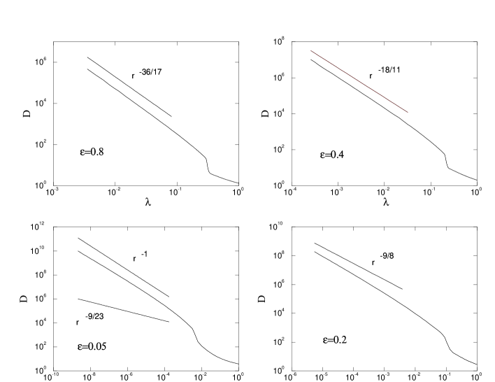
Figure 2: Density profiles obtained for $\epsilon=$0.8, 0.6, 0.4 and 0.05 by our hydrodynamical code, as a fonction of the self–similar radius $\lambda=r/r_{*}(t)$. The straight line in each graph is the power law predicted by the analytical calculations performed in this paper.

In figure (1), we plot the mass, density, velocity and pressure profiles obtained for the $\epsilon=1$ run. We compare our results with the semi-analytical profiles obtained by Bertschinger (1985). Note that both results agree remarkably well. Moreover, the computed shock front position is recovered within 3% accuracy. In figure (2), we plot the density profiles obtained for $\epsilon$ = 0.8, 0.6, 0.4 and 0.05. The straight line shows in each graph the corresponding asymptotic power law derived analytically in the last section. The numerical results agree perfectly well with the analytical ones. The $\epsilon=0.05$ case illustrates the change of behavior in the halo dynamics ($\epsilon\leq 1/6$). The power law $\rho\propto 1/r$ is very well recovered. We list in table (1) the shock front position $\lambda_{s}$ computed by our hydrodynamical code. Note that for lower $\epsilon$, the shock front is located at a much deeper radius.

5 DISCUSSION

We now discuss possible applications of our results on cosmic structures formation theory. We discuss here three major consequences of our work : an origin for segregation between gas and dark matter in X-ray clusters (David et al. 1996), an explanation of the Navarro et al. (1996) density profile and a justification for the stable clustering hypothesis.

5.1 Mass Distribution in the Core of X-Ray Clusters

The first application of the present work is to propose an interpretation of Navarro et al. (1996) dark matter density profile found with high resolution N-body simulations (see eq. [1]). This profile scales as $r^{-1}$ in the center of the cluster, as $r^{-2}$ for a large range of intermediate radii and as $r^{-3}$ in the outer regions. The outer regime, located roughly at the Virial radius, is likely to be the relaxation layer where shell crossings dominate, which leads to a profile steeper than isothermal. The intermediate power law ($r^{-2}$) is expected from the analytical approach for $\epsilon\leq 2/3$ and for purely radial orbits. Moreover, Tormen, Bouchet & White (1996) recently studied the distribution function in velocity space of simulated dark matter halos. They calculate for that purpose the factor $\beta(r)=1-\sigma^{2}_{t}/2\sigma^{2}_{r}$ where $\sigma_{t}$ and $\sigma_{r}$ are respectively the tangential and the radial velocity dispersion at a given radius. $\beta=1$ corresponds to purely radial orbits; $\beta=0$ to isotropic orbits and $\beta=-\infty$ to purely circular orbits. In the region where the density scales as $r^{-2}$, they found $\beta\simeq 1$, while in the central region, where the density scales as $r^{-1}$, they found $\beta\simeq 0$. In this paper, we show that for $\beta=1$, the flattest stable density profile is $r^{-2}$, and for the gas, which has $\beta=0$, the flattest stable density profile is $r^{-1}$. The results presented in this paper suggest that the change of slope in the density profile may be due to a change of dimensionality in the dark matter velocity space.

5.2 Segregation between Gas and Dark Matter

We showed that for $\epsilon\leq 2/3$, the density profiles obtained in the pure dark matter case differ from those obtained in the pure gas collapse. In cosmic structures, we expect both fluids (gas and dark matter) to be dynamically important. Therefore, the coupled dynamics has to be studied in order to have definitive answers. We have not been able to solve here analytically the coupled case, mainly because self-similarity is broken by the presence of two distinct fluids. The total mass profile is however expected to have a power law, between the pure gas and the pure dark matter profiles with $3/(1+3\epsilon)<\gamma<1$. The exact value of $\gamma$ depends on the value of $\Omega_{B}$, the universal gas fraction. In Chièze et al. (1996), we study the case of the single spherical Fourier mode. It can be shown that this corresponds to $\epsilon=4/9$. As expected, we obtain a segregation which depends on the chosen value of $\Omega_{B}$. Bertschinger (1985) studied the case $\epsilon=1$ in the coupled case, assuming a very low value for $\Omega_{B}$. As expected, he found no segregation. Our belief is that there is always a segregation between gas and dark matter for $\epsilon\leq 2/3$, and no segregation for $\epsilon\geq 2/3$. This would be due to the fact that the dark matter evolution is not strictly stationnary in the halo. This results in a systematic delay of gas shells relative to dark matter shells. Following Hoffman & Shaham (1985), it is possible to find the most probable initial density profile around a peak in the initial Gaussian random field. This leads to a power law initial perturbation which is roughly proportional to the linear two–point correlation function with $\epsilon=(n+3)/3$. We propose here that power spectra with $n\leq-1$ lead to segregation between gas and dark matter, with a dark matter density profile $\rho\propto r^{-2}$ and a gas density profile slightly shallower. However, if $n\geq-1$, gas and dark matter are expected to have similar density profiles with $\rho\propto r^{-9\epsilon/(1+3\epsilon)}$. This rather strong prediction has to be tested in 3D hydrodynamical simulations. Anninos & Norman (1996) found no significant segregation in their 3D simulations. They used a standard CDM power spectrum where $-1<n<0$ on clusters scales. Moreover, they found that the halo density profiles are well fitted by a $r^{-9/4}$ power law, both for gas and dark matter.

5.3 Stable Clustering Hypothesis

The last consequence of our work concerns one of the most powerful analytical prediction in gravitational dynamics, namely the stable clustering ansatz (Peebles 1980). This hypothesis states that on small scales the relative pair velocity cancels exactly the Hubble flow. For scale-free power spectra, this leads to the non-linear two-point correlation function $\xi\propto r^{-\gamma}$ with $\gamma=(9+3n)/(5+n)$. This regime is valid for $\xi\gg 1$ and has been extensively tested by N-body simulations (Jain 1996). Padmanabhan et al. (1995) try to find another derivation of the stable clustering hypothesis using the secondary infall model (which is the main topic of our paper). Instead of the linear two-point correlation function, they used for the initial spherical perturbation the smoothed r.m.s. density contrast. This leads to $\epsilon=(n+3)/6$. Using the solution of Fillmore & Goldreich (1984), the resulting halo profiles are (Jain 1996)

$$n\geq 1~{}~{}~{}~{}\rho\propto r^{-(9+3n)/(5+n)}$$

$$n<1~{}~{}~{}~{}\rho\propto r^{-2}$$

The next step is to assume that the two-point correlation function in the highly non-linear regime is dominated by the density field of such spherical halos. This has led Jain (1996) to conclude that the stable clustering hypothesis might be invalid for $n<1$. However, Fillmore & Goldreich (1984) results apply only for purely radial orbits. Therefore, the stable clustering regime might be recovered within a fully 3D density field. We saw in section 5.1 that recent N-body experiments suggest that on very small scales the distribution of dark matter particles is nearly isotropic in velocity space. Therefore, to derive the halo profiles using the initial conditions of Padmanabhan et al. (1995), one has to use the new solutions we found in this paper. This reads

$$n\geq-2~{}~{}~{}~{}\rho\propto r^{-(9+3n)/(5+n)}$$

$$n<-2~{}~{}~{}~{}\rho\propto r^{-1}$$

Therefore, assuming that the two-point correlation function is dominated in the highly non-linear regime by the density profiles of quasi-spherical halos with an isotropic distribution of particles in velocity space, one could justify the stable clustering hypothesis for $n\geq-2$. Significant deviation could be detected for $n=-2.5$, but this rather flat power spectra might be difficult to study using N-body simulations.

5.4 Conclusions

In this paper, we derive analytically gas and dark matter self-similar solutions for the gravitational collapse of a spherical perturbation embedded in an expanding Universe. The gas self-similar solutions can be easily extended to dark matter particles with an isotropic distribution in velocity space. The behavior of the gas differs from the dark matter one, leading to different results for each fluid. We find three possible consequences of our work : a possible segregation between gas and dark matter for a certain class of initial conditions ($\epsilon\leq 2/3$), a possible explanation for a dark matter density profile $\rho\propto r^{-1}$ in the central region of cosmic structures, and a possible justification of the stable clustering hypothesis for power spectra with $n\geq-2$.

$\epsilon$	1	0.8	0.6	0.4	0.2	0.05
$\lambda_{s}$	0.36	0.33	0.29	0.23	0.13	6.2$\times 10^{-3}$
$\Delta\lambda_{s}$	0.01	0.01	0.01	0.01	0.02	3.0$\times 10^{-3}$

Table 1: Self similar radius of the shock front and the corresponding uncertainties due to finite resolution obtained for different values of $\epsilon$ by our hydrodynamical code.

Figure 1: Density, pressure, velocity and mass profiles obtained in the $\epsilon=1$ case for the pure gas collapse, as a fonction of the self–similar radius $\lambda=r/r_{*}(t)$ (see text). Solid lines are the results obtained by Bertschinger (1985) using a semi-analytical method. Open circle are the results obtained by our hydrodynamical code. Both results agree perfectly well.

References

- Anninos & Norman (1996) Anninos, P.A., & Norman, M.L., 1996, ApJ, 459, 12
- Bertschinger (1985) Bertschinger, E., 1985, ApJS, 58, 39
- Binney & Tremaine (1987) Binney J., & Tremaine S., 1984, Galactic Dynamics, Princeton University Press
- Chièze, Teyssier and Alimi (1996) Chièze, J.-P., Teyssier, R., & Alimi, J.-M., 1996, submitted to ApJ.
- David, Jones & Forman (1995) David, L.P., Jones, C., & Forman, W., 1995, ApJ, 445, 578.