PKS 0116+082: An Optically Variable Compact Steep-Spectrum Source in an NLRG

Abstract

Polarimetry of the narrow-line radio galaxy PKS 0116+082 at the W.M. Keck telescope shows that it has high and variable optical polarization, presumably due to synchrotron radiation. It is not a BL Lac object because it has strong narrow lines, and it is not an OVV quasar because it has no broad lines and the extended galaxy is prominent. VLA and VLBA images show that it is a compact steep-spectrum radio source with most of the emission coming from a region less than 100 milli-arcsec in size. Of the 25 compact steep-spectrum or gigahertz peaked-spectrum sources measured polarimetrically, four have high optical polarization. One of these has been observed only once but in the other three the polarization is variable. This gives an intriguing hint that variability may be a general property of these objects.

1 Introduction

We have been measuring the polarization of radio galaxies with the W. M. Keck telescope, to study the alignment effect, the composition and disposition of material around the nucleus, the redshift dependence of the polarization, and the possible unification of narrow- and broad-line radio galaxies (NLRG and BLRG). For a general review of these topics see McCarthy (1993). As part of our study we observed the galaxy associated with the radio source PKS 0116+082 (J0119+0829). This source was identified with a distant galaxy by Spinrad et al. (1967) with $z=0.594$ and $m_{v}=20.7$, and spectroscopically is an NLRG. The optical radiation shows high polarization, as measured by Tadhunter et al. (1992) who found $p=5.4\%\pm 0.6\%$ at position angle $\theta=75\arcdeg\pm 3\arcdeg$, in the $V^{\prime}$ band (approximately 4885 – 6235 Å).

The radio source has not been well-studied; e.g., it has no VLA or VLBI images in the literature. However, it does display strong interplanetary scintillations, and therefore must be compact on a scale of one arcsecond. Harris & Gundermann Hardebeck (1969) showed that most of the source must lie within $0.05^{\prime\prime}$ at 408 MHz, and Readhead & Hewish (1974) showed that at least 0.65 of the flux comes from within $0.45^{\prime\prime}$ at 81.5 MHz. This object clearly is different from most other high-redshift radio galaxies (HZRG), in which most of the radio flux comes from extended radio lobes that have conspicuous hot spots near their outer edges (FRII morphology).

PKS 0116+082 may have flux variations of order 20% at centimeter wavelengths (Gregory & Condon (1991); Griffith et al. (1995)), but there is no evidence for large or rapid fluctuations. The spectrum is straight from 100 to 10,000 Mhz, with an index $\alpha=-0.52$ ($F_{\nu}\sim\nu^{\alpha}$; Kühr et al. (1981)). There is no suggestion of flattening at high frequencies, although there may be a steepening below 100 MHz. This index puts the source on the boundary between “steep” and “flat” spectrum objects. It appears to belong to the category generally designated as “compact steep-spectrum” (CSS; see e.g., O’Dea, Baum & Stanghellini (1991)). In these objects nearly all the radio emission arises within the host galaxy, although the radio image typically resembles that of the larger sources. A small fraction of CSS objects has complex or “two-dimensional” structure (Sanghera et al. (1995)), as does PKS 0116+082 (see below). It is thought that this compact complex structure arises from interactions between a radio-emitting relativistic jet and a dense interstellar medium near the nucleus of the galaxy (e.g., Wilkinson et al. (1991)).

Although there are no published VLA images of PKS 0116+082, this object indeed has been observed with the VLA, on several occasions. W. Coles and R. Grall observed it in 1990 May and June, and have kindly shared their original data with us. We show the first VLA images below. In addition, A. Beasley was able to obtain a VLBA³ snapshot for us and that is presented below also. These results show that the radio designation CSS is correct.

Our optical observations, described below, show that the optical polarization is strongly variable. This seems surprising because PKS 0116+082 is not BL Lac-like with very weak lines, nor is it quasar-like with broad emission lines and little or no starlight. However, little is known about the polarization of CSS objects, and the similar gigahertz peaked-spectrum (GPS) objects. In Section 4 we discuss the relation of PKS 0116+082 to other CSS/GPS objects.

In this paper we assume $\rm{H_{o}}=65~{}km~{}sec^{-1}~{}Mpc^{-1}$ and $\rm{q_{o}}=0.5$.

2 Optical Observations

a) Observations

We measured the polarization of PKS 0116+082 using the Low-Resolution Imaging Spectroscope (LRIS, Oke et al. (1995)) on the 10-m telescope at the W.M. Keck Observatory. The instrument contains a beamsplitter giving simultaneous measurements in orthogonal linear polarizations, and uses a half-wave plate set successively to four position angles, 0$\arcdeg$, 45$\arcdeg$, 22.5$\arcdeg$, and 67.5$\arcdeg$ as described by Goodrich (1991). Further aspects of the polarimeter are given by Goodrich, Cohen & Putney (1995), and in Appendix A. Table 1 gives the journal of observations. For spectroscopy we used a 300 g/mm grating blazed at 5000Å, which gives a resolution of 10Å with the 1^′′ slit and 15Å with the 1.5^′′  slit. Flux calibration was done with various standard stars: GD 248, G 193–74, G 191B2B, Feige 34, and Feige 110. Assorted clouds and highly variable seeing made most of the nights far from photometric.

For epochs 4a and 4b (Table 1) we replaced the grating in LRIS with a plane mirror and made imaging polarimetric observations through a Johnson $B$ filter. Unpolarized standard stars (e.g., Schmidt, Elston & Lupie (1992)) could not be used for primary calibration because they are too bright, and we tested the imaging polarimetry with stars 137 and 139 in the field Landolt 95 (Landolt (1992)). These stars have $B$ magnitudes 15.86 and 13.12 respectively. In high and variable seeing we measured, through the polarimeter, a flux ratio of $2.78\pm 0.02$ mag, which is in good agreement with Landolt’s values. We observed this field both with and without the UV calibration polarizer, and the polarization of the stars was measured by summing the appropriate fluxes in a square 3^′′ on edge and then calculating the Stokes parameters. With the polarizer stars 137 and 139 gave $p=99.5\%\pm 0.2\%$ and $99.9\%\pm 0.1\%$, respectively. Without the polarizer they gave $p=0.0\%\pm 0.16\%$ and $0.2\%\pm 0.04\%$, respectively. The errors are calculated from photon statistics. The galactic latitude of Landolt 95 is $-37\arcdeg$, sufficiently high that it is unlikely that interstellar polarization had any appreciable effect on these measurements. While there is no guarantee that the Landolt standards have low polarization, it is unlikely that they would be significantly polarized at a level and angle which would cancel any instrumental polarization. It is more likely that both the instrumental polarization and the polarization of the Landolt stars are near zero. The system is working properly at the extremes of 0% and 100% polarization.

The seeing was poor and variable during the 1995 December run, particularly for the observations of Landolt 95. Nonetheless, the polarimetry gives good results. This is because a dual-beam polarimeter is robust against seeing and transparency variations, provided an appropriate reduction algorithm is used. See Appendix A for a discussion of this point.

b) Spectropolarimetry Results

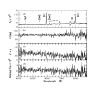
Figure 1: PKS 0116+082, 1995 December 17. (a) Total Flux. The atmospheric absorption bands (A, B, water vapor) have not been removed. (b) Position Angle $\theta$ (c) Fractional Linear Polarization, calculated as the “rotated Stokes parameter” (d) Polarized Flux = product of (a) and (c). The Total Flux (a) is shown at the original dispersion, 2.49 Å per pixel. Frames (b), (c) and (d) are calculated from fluxes which were binned by 4 pixels. Note the high continuum polarization in the blue, and the lack of polarization in the emission lines.

We have evidence that the polarization in PKS 0116+082 is variable (Section 2d) and hence do not combine data from different epochs. In Figure 1 we show the flux and polarization data for epoch 5a, which has the highest signal-to-noise ratio (S/N). The spectrum in Figure 1a is that of a typical NLRG. Gelderman & Whittle (1994) studied the optical spectra of a sample of 19 CSS sources, with the view of comparing them with other categories of objects and testing the idea that the small size is connected with an interaction between the interstellar medium and a relativistic jet. In all but one of Gelderman and Whittle’s objects [OIII]5007/H$\beta>>1$ as in Figure 1a, but in those objects where both [OII] and [OIII] are seen only one of ten has [OII]3727/[OIII]$5007>1$. PKS 0116+082 appears to have somewhat lower ionization than the typical CSS source.

In Figure 1b,c,d the fluxes were binned by 4 pixels to improve the S/N, and then the polarization parameters were calculated. Figure 1b shows the position angle $\theta$ which is independent of $\lambda$ from 4200 to 7600 Å  and has a mean value $\langle\theta\rangle=102.4\arcdeg\pm 0.6\arcdeg$. Figure 1c shows the “rotated Stokes parameter” $q^{\prime}$ which is an estimate of the true linear polarization $p$ obtained by rotating $q$ and $u$ by –204.8$\arcdeg$ (see Appendix A). The polarized flux (Fig 1d, the product of Figs 1a and 1c) is smooth and rises to the blue with a spectral index $\alpha\approx-1.5$. Note that the narrow lines do not appear in the polarized flux, indicating that they are unpolarized. This can also be seen in Figure 1c where $p$ drops to a low level in the [OII] line. The formal polarization of the [OII] line is $p([\rm{OII}])=0.4\%\pm 0.6\%$.

In Figure 1a several prominent galactic absorption lines are seen. We used a Keck spectrum of NGC 6702 as a template and found that the galaxy fraction is $29\%\pm 2\%$ at $\lambda_{\rm rest}=4600$Å, and about 12% near $\lambda_{\rm rest}=3727$Å. The AGN component (total – galaxy) has $p=4.9\%/0.71=6.9\%$ at $\lambda_{\rm rest}=4600$Å and $p=7.3\%/0.88=8.3\%$ at $\lambda_{\rm rest}=3727$Å. This suggests that $p$(AGN) rises to the blue, but the errors inherent in this calculation are fairly large, and the increase may not be real. In any event, the apparent increase in $p$ to the blue, seen in Fig. 1c, is largely due to the decrease in galaxy dilution.

The spectra of total and polarized flux show no significant broad H$\beta$ or Mg II emission, although the galaxy–subtracted spectrum (the AGN spectrum) gives a weak hint of broad H$\beta$. The best way to test for broad lines would be to look for H$\alpha$, at 1.05 microns.

c) Imaging Polarimetry Results

Figure 2 shows the $B$ band polarization image of PKS 0116+082, made by combining the data from epochs 4a and 4b. The data are binned 2x2 so that each pixel is 0.43^′′ square. Only those polarization vectors with $\rm{S/N}>2.0$ are shown. The strongest of the faint objects to the north has a formal debiased polarization $p=0.8\pm 0.9\%$, and the NW object has $p=0.1\%\pm 0.1\%$. These low values are consistent with these two objects being unpolarized, and give confidence that the system is working properly.

Note in Figure 2 that the polarization is uniform across the bright central part of the galaxy, as expected for a point source broadened by seeing. The PSF’s of PKS 0116+082 and the NW object are approximately equal, with FWHM=1.1^′′. This galaxy does not show the polarized extensions which are common in other HZRG. (See e.g., Tadhunter et al. 1992; di Serego Allighieri, Cimatti & Fosbury (1994); Januzzi et al. (1995).) The central square 2.4^′′ of PKS 0116+082 has $p=15.9\%\pm 0.2\%$ and $\theta=93.2\arcdeg\pm 0.2\arcdeg$. Both $p$ and $\theta$ are substantially different from their 1991 values, as reported by Tadhunter et al. (1992). This source is clearly variable, and in the next section we present all our data and discuss the variability.

d) Polarization Variability

In Table 2 we list our polarization measurements, and also the values given by Tadhunter et al. (1992) from their observations in 1991. The values for the imaging data were obtained by summing the fluxes in a box which simulates the spectral extraction window, and then calculating the Stokes parameters. The values for the spectroscopic data were made by similarly summing in wavelength to simulate $B$ and $V$ bands. Clearly these simulations are not exact, but tests of small changes in the windows produced only small changes in $p$ and $\theta$, less than the stated errors. The observations for epoch 2 were taken through clouds and the data below about 4600Å are not reliable. Our spectroscopic observations in 1994 were taken with a 1^′′ slit and those in 1995 with a 1.5^′′ slit. Dilution of the polarization by starlight or by any extended unpolarized component would cause $p$ to be smaller in 1995 than in 1994, contrary to what we observed. Further, slit width combined with dilution cannot change $\theta$ because Figure 2 shows that $\theta$ is essentially constant across the central region.

Table 2 shows that $p$ had about the same values in 1991 and 1994 and that there is little significant difference between the $B$ and $V$ band values. However, the temporal changes in $\theta$ are highly significant. In 1995 the values of $p$ and $\theta$ from measurement sets one hour apart (a and b) show changes; but these, we suspect, show that the errors (calculated from the photon statistics) are underestimated. However, the decrease in $p$ from epoch 4 to epoch 5, one day later, is surely significant; and the change in $\theta$ is also significant, but at a lower level.

The high value of $p$ from the imaging data, especially when compared with the spectral data for the following night, calls for a rigorous test of the system and the reduction procedure before the results can be fully accepted. A strong test is to compare the imaging data with spectral data taken on other occasions. We observed six objects in imaging mode on 1995 December 16. Four of the six have values of $(p,\theta)$ which agree with our spectropolarimetry to within $(0.4\%,2.3\arcdeg)$. One has $\Delta p\approx 0.3\%$ and $\Delta\theta\approx 6\arcdeg$. The sixth, PKS 0116+082, is much more discordant. We conclude that the data are trustworthy, and that the polarization of PKS 0116+082 changed strongly in one day.

Additional evidence of variability comes from the equivalent widths. Table 2 lists the rest-frame equivalent widths W_λ of the [OII] $\lambda 3727$ lines, in Angstroms. The 1995 values are significantly smaller than those from 1994. The differing slit widths in principle could affect W_λ because the starlight and [OII] emission could be extended but the UV continuum might be point-like. However we think this effect is small because seeing could similarly cause changes in W_λ, but no changes are seen between epochs 5a and 5b. It is clear that W_λ([OII]) decreased from 1994 to 1995, while $p$ increased.

From the polarization and the [OII] equivalent width we calculate $F^{\prime}_{c}$, the AGN continuum flux relative to the integrated [OII] flux (times 10,000), and $p_{c}$, the polarization of the AGN continuum at 3727Å. In doing this we assume that the [OII] flux is constant and that the galaxy component is constant and unpolarized. The appropriate formulae are

$$p_{c}={p\over{1-g}};~{}~{}~{}~{}~{}~{}~{}F^{\prime}_{c}\sim{F_{c}\over\rm[OII]}={{1-g}\over\rm W}$$

where $g$ is the galaxy fraction at 3727Å  and W is the equivalent width of [OII]. For earlier epochs when the galaxy fraction could not be accurately measured, we replace $g$ with $g_{5}(\rm{W/W_{5}})$, where $g_{5}$ and $\rm{W_{5}}$ are measured at epoch 5a. $F^{\prime}_{c}$ and $p_{c}$ are given in Table 2, columns 7 and 8. From 1994 to 1995 the AGN flux increased by about 30%, and the polarization from about 6% to 9%.

Note that the implied equivalent widths of the emission lines are well within the normal observed range for AGN (e.g., Dahari & De Robertis (1988)); there is no evidence for a deficit of ionizing photons from the line strengths. This is especially true given the steepness of the galaxy-corrected continuum, $\alpha=0.72$.

3 Radio Observations

PKS 0116+082 was observed for an unrelated project at the VLA by W. Coles and R. Grall in 1990 May and June at three frequencies, 1.7, 5.0, and 8.5 GHz, in A configuration with 50 MHz bandwidth, in single scans of duration 70, 90, and 100 sec at the three frequencies, respectively. Coles and Grall have kindly shared their original data with us, and we produced images from them. The brief snapshots have poor dynamic range, but the resulting images are adequate to obtain a reasonable idea of the shape of the source and its orientation. Two 8.5 GHz images are shown in Figure 3. The “tapered” map (giving maximum sensitivity to extended emission) in Figure 3a shows a weak component to the east extending about $2^{\prime\prime}$. The “uniformly-weighted” map in Fig. 3b (giving maximum angular resolution at the expense of dynamic range) shows a faint extension to the west and, in addition, this image shows a more prominent extension to the north-west, close to the center. Model-fitting two circular Gaussians to the inner extension gives component strengths of 0.52 and 0.14 Jy. Their sizes are not well-constrained but they are separated by $\sim$225 milli-arcsec (mas) ($\sim$1 beamwidth) in position angle $-47\arcdeg$. The 5.0 GHz observations also show both an eastern and a (north)western extension, but the inner double is not well resolved. The observations at 1.7 GHz clearly show only the eastern extension. These results show that PKS 0116+082 is compact at centimeter wavelengths, with nearly all the flux arising within 1 arcsec. This confirms the results from interplanetary scintillations.

PKS 0116+082 was observed at the VLBA by A. Beasley at 1.7 GHz on 1996 March 14. The observation consisted of one 5-minute snapshot, and the resulting image, shown in Fig. 4a, has only a modest dynamic range. The source was then included by RCV in an unrelated multi-snapshot VLBA survey at 5.0 GHz, observed on 1996 August 22. The image, which is essentially thermal noise limited, is shown in Fig. 4b.

The images show an elongated curved structure, with an overall length of about 75 mas, or 0.5 kpc. The nucleus is probably in the northernmost, most compact component. This feature has an inverted spectrum and is not the strongest one even at 5.0 GHz, presumably due at least in part to synchrotron self-absorption. The brightest component at both frequencies occurs south of the gap, and seems to mark the onset of a region of strong curvature, in which the jet definitely becomes resolved transversely. Afterwards, the jet points almost directly at the knot seen with the VLA (Fig. 3b) at a projected distance of 225 mas.

a) A New Radio Position

The 8.5 GHz VLA observations allow us to calculate a new radio position for the source, given in Table 3. This position was obtained by model-fitting to the pre-selfcalibrated VLA data, which were calibrated with the astrometric calibrator J0149+059 (Johnston et al. (1995)). Model-fitting errors are about 0.02^′′ and the phase transfer errors are probably of similar magnitude; we estimate the positional errors in both RA and Dec to be about 0.035^′′. Table 3 also contains the Spinrad et al. (1967) value for the optical position, precessed to J2000 coordinates. The radio and optical positions agree to within the stated error in the optical position.

4 Discussion

a) Classification of PKS 0116+082

PKS 0116+082 is in an NLRG displaying rapid optical polarization variability. The two classes of objects with such variability are BL Lac objects and optical violently variable (OVV) quasars, but PKS 0116+082 cannot be placed in either one. The definitions of these classes are not tight because observers emphasize different characteristics, which themselves generally have a broad distribution. Furthermore, some objects have ambiguous classifications because their variability carries them from one class to another. We shall borrow from the discussion of Januzzi, Smith & Elston (1993) who, in a discussion of X-ray selected BL Lac objects, reviewed the history of the definitions of some of the AGN classes. A BL Lacertae object, according to Januzzi et al., is an object with (1) strong and rapid variability, (2) a “featureless” optical spectrum (W${}_{\lambda}<5$Å), and (3) high linear polarization. A highly-polarized quasar (HPQ) is a quasar with optical polarization $p>3\%$. An OVV quasar displays rapid and large changes in flux density. It appears that all OVV quasars are also HPQ’s, but the converse is not true. A blazar is any object which is violently variable in flux and has high and variable optical polarization. Blazar is a general term which includes BL Lacs and OVVs even though these typically have very different luminosities.

The important feature of PKS 0116+082 is that it has strongly variable optical polarization. However it does not appear to have strong radio variability, so it is not a blazar. It is not a BL Lac because it has strong narrow lines and it is not a quasar because it is clearly extended, and furthermore any broad lines are very weak. It cannot be classified in the conventional way.

b) Origin of the Polarization

The optical light from AGN can be polarized by selective absorption in aligned dust grains, by scattering from electrons or dust, and by the synchrotron effect. Dust absorption appears to be ruled out in PKS 0116+082 because the high polarization (16%) is extreme for dust absorption, and because polarization due to this mechanism cannot vary on short time scales. Similarly, although polarization caused by scattering off dust or electrons can easily reach the high values seen in PKS 0116+082, it cannot easily have a position angle which varies on short time scales. We therefore propose that the polarization in PKS 0116+082 is due to synchrotron radiation. The lack of polarization in the emission lines (Section 2b) is consistent with this interpretation.

The optical synchrotron source must lie well inside the radio synchrotron source, because it requires a combination of higher density and stronger magnetic field. The variation in one day implies that it is not larger than about $3\times 10^{15}$ cm in extent. This estimate is too small if the optically emitting synchrotron material itself has an outward bulk relativistic motion.

c) Relation to Other CSS/GPS Sources

CSS radio sources are compact and have a steep spectrum. The GPS radio sources are similar except that their spectrum has a peak around 1 GHz. The peak is presumably due to synchrotron self-absorption, and the only distinction between the two classes seems to be that the GPS sources have higher optical depth to synchrotron radiation. We can consider the CSS and GPS sources together.

About 150 CSS/GPS sources are known (Dallacassa & Stanghellini (1990), O’Dea, Baum & Stanghellini (1991)), and we have found optical polarization measurements for 25 of them in the literature (Impey & Tapia (1990), Impey, Lawrence & Tapia (1991), Tadhunter, Shaw & Morganti (1994), Xu (1995), and our unpublished Keck data). 8/25 are definitely polarized ($p\geq 3\sigma$) and 4/8 are highly polarized ($p\geq 3\%$). Most of the measured objects are quasars (22/25) and the remaining 3 are NLRG. Of the highly-polarized objects, 2 are quasars and 2 are NLRG. The fraction of HPQ among the quasars (2/22) appears to be smaller than the HPQ fraction (0.3) found by Impey and Tapia, but most of the quasars in our list were only observed once and the fraction would surely increase if a serious measurement campaign were made.

The two HPQs are 3C 216 and CTA 102. 3C 216 (z=0.67) originally was called a BL Lac object but then was labelled a quasar by Smith & Spinrad (1980) because it showed substantial [OII]$\lambda$3727 and, perhaps, broad MgII $\lambda$2800. Lawrence et al. (1996), with a better spectrum, list the equivalent widths of [OII]$\lambda 3727$ and [OIII]$\lambda 5007$ as 15.5 and 13.0 Å, respectively, which are larger than the usual BL Lac limit, 5Å. The FWHM of MgII and H$\beta$ are both 1800 km sec^-1 which is intermediate between “narrow” and “broad”. At radio wavelengths 3C 216 is a CSS object containing superluminal components (Barthel, Pearson & Readhead (1988)) but, like PKS 0116+082, it is not a rapid variable and would not be called a blazar. Its optical polarization is variable (Kinman (1976)), with maximum 21%.

CTA 102 (z=1.037) also has variable optical polarization (Impey & Tapia (1990)) with maximum 10.9%. At centimeter and meter wavelengths its flux has slow variations. The existence of superluminal motion in CTA 102 has been debated (Wehrle & Cohen (1989), Rantakyro et al. (1996)), but there is no doubt that CTA 102 contains a powerful radio jet. It is also a $\gamma$–ray source (Thompson et al. (1995)).

The two highly-polarized NLRG are PKS 0116+082 and PKS 1934–638. Tadhunter, Shaw & Morganti (1994) showed that PKS 1934–638 ($z=0.183)$ has strong optical polarization in the $B$ band, 4% in a small aperture and perhaps as much as 7% for the featureless continuum alone. It has only been observed once, as far as we are aware, so that its variability is unknown. Fosbury et al. (1987) discussed its spectrum; it has strong narrow lines which on analysis show that the electron density is higher than usual for NLRG. The radio morphology is double, with an exceptionally large ratio of separation to size. There is no superluminal motion (Tzioumis et al. (1989)).

PKS 0116+082 and PKS 1934–638 have similar optical spectra and both are highly-polarized. They are compact at radio wavelengths but the detailed small-scale structure is different. PKS 0116+082 is complex, whereas PKS 1934–638 is a stationary double with a large ratio of separation to size; these differences may reflect the density and complexity of the ISM near the galactic nucleus. All three of the well-measured highly polarized CSS/GPS objects show strongly variable polarization. It will be interesting to measure the fourth object, PKS 1934–638, to see if it, too, is variable.

d) Nature of PKS 0116+082

We first ask if the unusual nature of PKS 0116+082 can result from an accidental close alignment of two objects; one a CSS source in an NLRG, and the other an optically variable object either in front of or behind the NLRG. The spectrum contains no hint of a second redshift system, so the variable object would have to be lineless; ie. a BL Lac object. We think this is highly unlikely because both CSS/GPS and BL Lac objects are rare. The similarity of PKS 0116+082 and PKS 1934–638 argues for a common mechanism, which makes the probability of chance alignments between the two rare classes vanishingly small.

The synchrotron origin for the polarization implies that the nucleus contains high-energy electrons in a magnetic field. The rapid variations mean that we probably are getting a direct view of this nuclear source rather than seeing it by reflection or through a cloud which would quench the rapid variations. On the other hand, many HZRG are believed to contain an opaque torus that confines the nuclear optical and UV light to oppositely directed “cones” of emission (e.g., IRAS 09104+4109, Hines & Wills (1993)). If PKS 0116+082 has such a torus then either we are looking close to the axis, or the torus has a “hole” through which we have a view of the central continuum source. In the former case we should also see any broad-line region (BLR) which exists near the nucleus, but we see little evidence for broad lines. In the latter case the hole could probably be arranged to exclude a BLR, but this seems contrived. We note that spectra of PKS 1934–638 (Fosbury et al. (1987)) also give no evidence of broad H$\alpha$ or H$\beta$. We suggest that the lack of observed broad lines in PKS 0116+082 is best interpreted as meaning that in fact there is no BLR, or at least that it is unusually weak. In this case it does not fit into the quasar/BLRG/NLRG unification scheme (e.g., Barthel (1989)).

We assumed above that the radio nucleus of PKS 0116+082 is the northern compact component, and described the structure as “core-jet” with a pronounced curvature beginning about 60 mas (400 pc, projected) from the nucleus. The one-sided nature of the jet is usually regarded as a sign of relativistically boosted synchrotron radiation, and this leads to limits on the Lorentz factor of the flow, $\gamma$, and the angle to the line of sight, $\phi$. For example, if the front-to-back ratio is 20 or more, then $\gamma>1.3$ and $\phi<50\arcdeg$, approximately. The strong curvature is also a sign of an end-on view, in which a modest curvature can be strongly amplified by projection. These factors argue that the radio jet is not close to the plane of the sky, say $\phi<50\arcdeg$. This reinforces the possibility that we are looking inside any central torus, and should see a broad emission-line region if it were there.

The three CSS/GPS objects with variable polarization are united by radio morphology and spectrum, but optically they include both quasars and narrow-line radio galaxies. Furthermore, in the case of PKS 0116+082, it appears doubtful that the RG/quasar unification-by-aspect is at work. Since the polarized CSS/GPS objects transcend both galaxies and quasars, and because their number is so small, it does not seem useful to try to define a new subclass for them. Further polarimetric observations would be useful in this regard.

5 Conclusions

1) PKS 0116+082 shows rapid variations in optical polarization, including a change from 16% to 9% in one day. The position angle has varied from $10\arcdeg$ to $103\arcdeg$ over a one-year period. Although our observations were typically not in photometric conditions, we were able to scale the polarized flux by assuming that the [OII]$\lambda 3727$ flux and the host galaxy flux are constant. From 1994 to 1995 the AGN continuum flux increased by about 30%, while the AGN polarization increased from about 6% to 9%.

2) PKS 0116+082 is a CSS radio source in an NLRG. The radio structure is compact and complex. We show the first VLA and VLBI images of this object.

3) The radio flux appears to have only modest variations. PKS 0116+082 is not a BL Lac object because it has strong narrow lines and it is not a HPQ because the host galaxy is prominent and there are no readily visible broad lines.

4) Of the approximately 150 known CSS/GPS sources, 25 have been observed polarimetrically. Four are known to be highly polarized at optical wavelengths. Three of the four have variable polarization and the fourth has been observed only once.

5) Our current data give little evidence for broad H$\beta$ or Mg II emission in the total or polarized flux from PKS 0116+082, although optical synchrotron radiation is seen. The most likely explanation for this is that any broad-emission-line region is exceptionally weak.

APPENDIX

Appendix A The LRIS Polarimeter

The LRIS polarimeter is a dual-beam instrument of the type first described by Miller, Robinson & Goodrich (1988) and further discussed by Goodrich (1991) and Goodrich, Cohen & Putney (1995). Our aim in this Appendix is to discuss the particular algorithm we use for reductions, and to demonstrate the robustness of the system. We use the Stokes Parameters I,Q and U and assume that the circular polarization parameter V is zero.

The polarimeter lies directly under the slit mask of the LRIS. For imaging the mask is removed and a mirror is substituted for the grating. The beam goes successively through a calibration wheel, a rotatable super-achromatic half-wave plate, and a calcite beamsplitter. The beamsplitter produces parallel orthogonally-polarized beams separated by $73^{\prime\prime}$ that go to the camera and make two images (spectra) on the CCD. The field of view is about 35^′′ square.

The fundamental assumption we make in analyzing the images is that the CCD counts are proportional to the linear Stokes parameters $\rm{I_{x}}$ and $\rm{I_{y}}$ at the top of the atmosphere, where $\rm{I_{x}}\equiv(I+Q)/2,\rm{I_{y}}\equiv(I-Q)/2$, and x and y are respectively the polarization directions of the ordinary and extraordinary (o and e) rays emerging from the beamsplitter. We then assume that the proportionality constants can be factored as follows. When the fast axis of the waveplate is set to $0\arcdeg$ (ie. parallel to the x-axis) we have

$$\rm{B_{0}=t_{0x}g_{0b}I_{x}}$$

$$\rm{T_{0}=t_{0y}g_{0t}I_{y}}$$

where B and T are the CCD counts in the images made by the o and e rays, respectively; t is the transmission coefficient to the beamsplitter and includes atmospheric opacity, telescope magnification, and the effects of seeing and guiding; and g is the overall gain in the optical path from the beamsplitter to the extracted CCD counts, including the effects of flat-fielding and sky subtraction. The subscript 0 stands for the angular orientation of the waveplate, and the subscripts b and t stand for the o and e rays and for the bottom and top spectra seen in the image displayed by VISTA.

After an exposure is made at $0\arcdeg$ we make another at $45\arcdeg$, giving

$$\rm{B_{45}=t_{45y}g_{45b}I_{y}}$$

$$\rm{T_{45}=t_{45x}g_{45t}I_{x}}$$

where we have assumed that the waveplate and the beamsplitter are perfect, so that a $45\arcdeg$ rotation interchanges $\rm{I_{x}}$ and $\rm{I_{y}}$. We now assume that there is no polarization dependence in the transmission coefficients: $\rm{t_{0x}=t_{0y}}$ and $\rm{t_{45x}=t_{45y}}$ , and that the instrumental gains do not change during the two exposures: $\rm{g_{0b}=g_{45b}}$ and $\rm{g_{0t}=g_{45t}}$. The four images or spectra can now be combined to give the following three independent quantities, in addition to the total intensity $\rm{I=I_{x}+I_{y}}$.

$$\Omega\equiv\sqrt{B_{0}T_{0}\over B_{45}T_{45}}={t_{0}\over t_{45}}$$

$$G\equiv\sqrt{B_{0}B_{45}\over T_{0}T_{45}}={g_{b}\over g_{t}}$$

$$q\equiv{{I_{x}-I_{y}}\over{I_{x}+I_{y}}}={{{\sqrt{B_{0}T_{45}}-\sqrt{B_{45}T_{0}}}\over{\sqrt{B_{0}T_{45}}+\sqrt{B_{45}T_{0}}}}}$$

Eq. (5) can also be written in the suggestive forms

$$q={{B_{0}-GT_{0}}\over{B_{0}+GT_{0}}}={{B_{0}-\Omega B_{45}}\over{B_{0}+\Omega B_{45}}}$$

The Stokes Parameter $u$ is similarly found, with waveplate settings at $22.5\arcdeg$ and $67.5\arcdeg$. Formulae 3–6 are the same as those described by Miller, Robinson & Goodrich (1988) although the symbols are different; our $\Omega$ is their $\omega$. Walsh (1992) describes a similar polarimeter and derives our Eq. (5) (his Eq. 7) but he does not explicitly discuss G or $\Omega$.

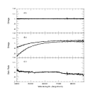
Figure 5: (a) $\Omega$ (Eq. 3) for Hiltner 102, 1994 August, four $20^{s}$ exposures taken in clear skies (b) $\Omega$ for Hiltner 102, 1994 October, four $15^{s}$ exposures taken through cirrus (c) G (Eq. 4) for Hiltner 102, 1994 August, four $20^{s}$ exposures.

The quantity $\Omega$ is the ratio of the transmission coefficients in the two exposures and is useful as a check on the observing conditions. Figure 5 shows $\Omega$ for the standard star Hiltner 102; Figure 5a was taken in good conditions and Figure 5b through cirrus. In both panels there are two curves, for the $q$ and $u$ observations. In the top panel the curves overlap. The middle panel is unusual in the wide separation between the two curves and the strong wavelength dependence, due to the changing atmosphere. In all cases $q$ and $u$ are taken successively and for the middle panel the total elapsed time was $147^{s}$. Figure 6 shows an imaging $\Omega$ for an exceptionally bad case, when the seeing was changing rapidly. The two exposures which are combined to make Figure 6 are each $5^{s}$ in duration and are separated by $65^{s}$. In the center $\Omega=3.3$, which shows that the seeing became much worse between the two exposures.

The quantity G is the gain ratio between the two beams and can be monitored as a check on the system and on the quality of spectral extraction. It has been observed to show variations during a night. Figure 5c shows a typical curve of G.

The normalized Stokes Parameter $q$ is given in Eq. 5 in terms of geometric means that explicitly show how the $t$’s and $g$’s cancel from each term in the numerator and denominator. The system is self-calibrated $at~{}each~{}pixel~{}in~{}an~{}image$ or $at~{}each~{}wavelength~{}in~{}an~{}extracted~{}spectrum$. The calculation is robust against seeing or opacity changes because each point has its own values of G and $\Omega$. For example, in spite of the poor sky so evident in Figs 5b and 6, the values of q and u obtained with those data were clean and were used as a check on the polarimeter performance.

When the seeing is changing (Fig 6) the calculated $q$ at each point involves a peculiar average over two different seeing disks. It is not necessary, however, to convolve the two images to the same psf to get reliable results. Note that Eq 5 involves small differences between large numbers, so that some care must be taken with the data. In particular, G and $\Omega$ should be calculated internally with the $q$ or $u$ data, and should not be taken from other exposures to be used with Eq. 6.

The electric vector of the incident light has a position angle $\theta=0.5\rm{arctan}(u/q)$. For a noise-free situation the fractional linear polarization $p$ is calculated as $p=\sqrt{q^{2}+u^{2}}$, but this gives a biased result when the S/N is low (S/N $<5$). In such cases various de-biasing schemes are available (see Simmons & Stewart (1985)). Our data on AGN usually show that $\theta$ varies slowly with $\lambda$ and so a good approximation to $p$ can be obtained by rotating $(q,u)$ by $-2\Theta$, where $\Theta$ is a smooth approximation to $\theta$. This gives $(q^{\prime},u^{\prime})$ where $q^{\prime}\approx p$ and $u^{\prime}\approx 0$. $|q^{\prime}|$ is biased low by approximately $cos2(\Theta-\theta)$. In our experience this often is preferable to debiasing the square-root formula (Stockman & Angel (1978)).

When the S/N is low the calculated values of $|q|$ and $|u|$ (Eq. 5) themselves are biased high (Clark et al. (1983)). In this case it is important to average the flux values to improve the S/N, and not to average the $(q,u)$ values.

Table 1: Journal of Observations.

Epoch	UT Date	Type	Exp	$\Delta\lambda$ (Å)	Slit	Comments
1	28/10/94	SPOL	4800	4000–9000	1	Clear
2	29/10/94	SPOL	6400	4000–9000	1	Cloudy
3	31/12/94	SPOL	2880	3900–8900	1	poor seeing
4a	16/12/95	IPOL	3600	$B$ Band		seeing $\sim 1.1^{\prime\prime}$
4b	16/12/95	IPOL	3600	$B$ Band		seeing $\sim 1.0^{\prime\prime}$
5a	17/12/95	SPOL	3600	3900–8900	1.5	seeing $\sim 0.8^{\prime\prime}$
5b	17/12/95	SPOL	3600	3900–8900	1.5	seeing $\sim 1.5^{\prime\prime}$

Table 2: Observations of PKS 0116+082.

Epoch	$p(\%)$	$\theta$ (deg)	$p(\%)$	$\theta$ (deg)	Wλ	$F_{c}^{\prime}$	$p_{c}$	Comments
Aug 91			$5.4\pm 0.6$	$75\pm 3$				Tadhunter $V^{\prime}$
1	$5.6\pm 0.3$	$13.5\pm 2.0$	$4.9\pm 0.2$	$8.4\pm 1.4$	124	69	6.0
2			$5.2\pm 0.2$	$10.5\pm 2.1$	118	73	6.3	cloudy
3	$5.8\pm 0.7$	$28.7\pm 2.4$	$4.3\pm 0.3$	$30.6\pm 1.9$	122	70	5.4
4a	$16.7\pm 0.1$	$94.9\pm 0.2$						IPOL $B$ Band
4b	$15.6\pm 0.2$	$91.0\pm 0.3$						IPOL $B$ Band
5a	$8.5\pm 0.3$	$102.0\pm 1.2$	$7.3\pm 0.2$	$102.1\pm 0.8$	99	89	8.8
5b	$8.9\pm 0.2$	$100.9\pm 2.0$	$7.0\pm 0.4$	$103.0\pm 1.6$	99	89	8.5	Seeing 1–2′′

Table 3: Positions of PKS 0116+082.

	RA (J2000)	$\pm$	Dec (J2000)	$\pm$
Radio	$01^{h}19^{m}01^{s}.275$	$0^{s}.003$	$+08\arcdeg 29^{\prime}54^{\prime\prime}.69$	$0^{\prime\prime}.035$
Optical	$01^{h}19^{m}01^{s}.28$	$0^{s}.03$	$+08\arcdeg 29^{\prime}54^{\prime\prime}.7$	$0^{\prime\prime}.5$

Figure 2: Polarization image for PKS 0116+082, 1995 December 16. Contour levels are 0.5,1,2,4,8,16,32,64% of the peak. The pixels are 0.43^′′ square, and only those vectors with $\rm{S/N}>2$ are plotted. The peak polarization vector near the flux peak has $p=17.3\%\pm 0.2\%$ at $\theta=96.7\arcdeg\pm 0.4\arcdeg$.

Figure 3a: VLA images of PKS 0116+082 at 8.5 GHz, observed on 1990 June 15. a) A tapered image, with a restoring beam of 0.83 by 0.76 arcsec in PA $-69\arcdeg$, emphasizing the extended emission. The contour levels increase in factors of 2, starting at 2.25 mJy/beam (3 times the r.m.s. noise in the image), with a peak of 794 mJy/beam.

Figure 3b: VLA images of PKS 0116+082 at 8.5 GHz, observed on 1990 June 15. b) Uniformly weighted image, giving maximum resolution, with a restoring beam of 0.38 by 0.28 arcsec in PA $57\arcdeg$, and contour levels starting at 3.26 mJy/beam and a peak of 630 mJy/beam.

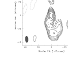
Figure 4a: Naturally weighted VLBA images of PKS 0116+082. a) at 1.7 GHz, observed on 1996 March 14, with a restoring beam of 9.5 by 4.2 milliarcsec in PA $4\arcdeg$. The contour levels increase in factors of 2, starting at 3.0 mJy/beam (3 times the r.m.s. noise in the image), with a peak of 362 mJy/beam.

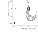
Figure 4b: Naturally weighted VLBA images of PKS 0116+082. b) at 5.0 GHz, observed on 1996 August 22 with a restoring beam of 4.0 by 2.0 milliarcsec in PA $6\arcdeg$. The contour levels increase in factors of 2, starting at 1.0 mJy/beam (3 times the r.m.s. noise in the image), with a peak of 183 mJy/beam.

Figure 6: $\Omega$ (Eq. 3) for star 139 in the field Landolt 95, 1995 December. The calculation uses two $5^{s}$ exposures separated by $75^{s}$. Contours 0.3, 0.5, 0.8, 1.5, 2.5, 3.3. The effect of a strong seeing change between the two exposures can be seen.

References

- Barthel (1989) Barthel, P.D. 1989, ApJ, 336, 606
- Barthel, Pearson & Readhead (1988) Barthel, P.D., Pearson, T.J., & Readhead, A.C.S. 1988, ApJ, 329, L51
- Clark et al. (1983) Clark D., Stewart, B.G., Schwartz, H.E., & Brooks, A. 1983, A&A, 126, 260
- Dallacassa & Stanghellini (1990) Dallacassa, D., & Stanghellini, C. 1990, in Compact Steep-Spectrum GHZ-Peaked Spectrum Radio Sources, ed C. Fanti, R. Fanti, C.P. O’Dea & R.T. Schillizi, Workshop held in Dwingeloo – The Netherlands on June 18-19, 1990 (CNR Istituto di Radioastronomia, Bologna), p224
- Dahari & De Robertis (1988) Dahari, O., & De Robertis, M. M. 1988, ApJS, 67, 249
- di Serego Allighieri, Cimatti & Fosbury (1994) di Serego Alighieri S., Cimatti, A., & Fosbury, R.A.E. 1994, ApJ, 431, 123
- Fosbury et al. (1987) Fosbury, R.A.E., Bird, M.C., Nicholson, W., & Wall, J.V. 1987, MNRAS, 225, 761
- Gelderman & Whittle (1994) Gelderman, R., & Whittle, M. 1994, ApJS, 91, 491
- Goodrich (1991) Goodrich, R.W. 1991, PASP, 103, 1314
- Goodrich, Cohen & Putney (1995) Goodrich, R.W., Cohen, M.H., & Putney, A. 1995, PASP, 107, 179
- Griffith et al. (1995) Griffith,M.R., Wright, A.E., Burke, B.F., & Ekers, R.D. 1995, ApJS, 97, 347
- Gregory & Condon (1991) Gregory, P.C., & Condon, J.J. 1991, ApJS, 75, 1011
- Harris & Gundermann Hardebeck (1969) Harris, D.E., & Gundermann Hardebeck E. 1969, ApJS, 19, 115
- Hines & Wills (1993) Hines, D.C. & Wills B.J. 1993, ApJ, 415, 82
- Impey & Tapia (1990) Impey, C.D., & Tapia, S. 1990, ApJ, 354, 124
- Impey, Lawrence & Tapia (1991) Impey, C.D., Lawrence, C.R., & Tapia, S. 1991, ApJ, 375, 46
- Januzzi, Smith & Elston (1993) Januzzi, B.T., Smith, P.S., & Elston, R. 1993, ApJS, 85, 265
- Januzzi et al. (1995) Januzzi, B.T., Elston, R., Schmidt, G.D., Smith, P.S., & Stockman, H.S. 1995, ApJ, 454, L111
- Johnston et al. (1995) Johnston, K.J. et al. 1995, AJ, 110, 880
- Kinman (1976) Kinman, T.D. 1976, ApJ, 205, 1
- Kühr et al. (1981) Kühr, H., Witzel, A., Pauliny-Toth, I.I.K., & Nauber, U. 1981, A&AS, 45, 367
- Landolt (1992) Landolt, A.U. 1992, AJ, 104, 340
- Lawrence et al. (1996) Lawrence, C.E., Zucker, J.R., Readhead, A.C.S., Unwin, S.C, Pearson, T.J., & Xu, W. 1996, ApJS, 107, 541
- McCarthy (1993) McCarthy, P.J. 1993, ARA&A, 31, 639
- Miller, Robinson & Goodrich (1988) Miller, J.S., Robinson, L.B., & Goodrich, R.W. 1988, in Instrumentation for Ground-Based Astronomy, ed. L.B. Robinson (New York, Springer), p157
- O’Dea, Baum & Stanghellini (1991) O’Dea, C.P., Baum, S.A., & Stanghellini, C. 1991, ApJ, 380, 66
- Oke et al. (1995) Oke, J.B., Cohen, J.G., Carr, M., Cromer, J., Dingizian, A., Harris, F.H., Labreque S., Lucinio, R., Schaal, W., Epps, H., & Miller, J. 1995, PASP, 107, 375
- Rantakyro et al. (1996) Rantakyro, F.T., Baath, L.B., Dallacasa, D., Jones, D.L., & Wehrle, A.E. 1996, A&A, 310, 66
- Readhead & Hewish (1974) Readhead, A.C.S., & Hewish A. 1974, MmRAS, 78, 1
- Simmons & Stewart (1985) Simmons, J.F.L., & Stewart, B.G. 1985, A&A, 172, L11
- Sanghera et al. (1995) Sanghera H.S., Sakia, D.J., Lüdke, E., Spencer, R.E., Foulsham, P.A., Akujor, C.E., & Tzioumis A.K. 1995, A&A, 295, 629
- Schmidt, Elston & Lupie (1992) Schmidt, G.D., Elston, R., & Lupie, O.L. 1992, AJ, 104, 1563
- Smith & Spinrad (1980) Smith, H.E., & Spinrad, H. 1980, ApJ, 236, 422
- Spinrad et al. (1967) Spinrad, H., Liebert, J., Smith, H.E., & Hunstead, R. 1967, ApJ, 206, L79
- Stockman & Angel (1978) Stockman, H. S., & Angel, J. R. P. 1978, ApJ, 220, L69
- Tadhunter et al. (1992) Tadhunter, C.N., Scarrott, S.M., Draper, P., & Rolph, C. 1992, MNRAS, 256, 53p
- Tadhunter, Shaw & Morganti (1994) Tadhunter, C.N., Shaw, M.A., & Morganti, R. 1994, MNRAS, 271, 807
- Thompson et al. (1995) Thompson, et al. 1995, ApJS, 101, 259
- Tzioumis et al. (1989) Tzioumis, A.K. et al. 1989, AJ, 98, 36
- Walsh (1992) Walsh, J.R. 1992, in ESO/ST-ECF Data Analysis Workshop ed P.J. Grosbol and R.C.E. de Ruijsscher, ESO Conf. and Workshop Proc. No. 41, p53
- Wehrle & Cohen (1989) Wehrle, A.E., & Cohen, M.H. 1989, ApJ, 346, L69
- Wilkinson et al. (1991) Wilkinson, P.N., Tzioumis, A.K., Benson, J.M., Walker, R.C., Simon, R.S., & Kahn, F.D. 1991, Nature, 352, 313
- Xu (1995) Xu, W. 1995, Ph.D. Thesis, California Institute of Technology