Constraints on $\Omega_{0}$ and Cluster Evolution using the ROSAT LogN–LogS

Abstract

We examine the likelihoods of different cosmological models and cluster evolutionary histories by comparing semi-analytical predictions of X-ray cluster number counts to observational data from the ROSAT satellite. We model cluster abundance as a function of mass and redshift using a Press-Schechter distribution, and assume the temperature $T(M,z)$ and bolometric luminosity $L_{X}(M,z)$ scale as power laws in mass and epoch, in order to construct expected counts as a function of X–ray flux. The $L_{x}-M$ scaling is fixed using the local luminosity function while the degree of evolution in the X-ray luminosity with redshift $L_{X}\!\propto\!(1+z)^{s}$ is left open, with $s$ an interesting free parameter which we investigate. We examine open and flat cosmologies with initial, scale–free fluctuation spectra having indices $n=0$, $-1$ and $-2$. An independent constraint arising from the slope of the luminosity–temperature relation strongly favors the $n\!=\!-2$ spectrum.

The expected counts demonstrate a strong dependence on $\Omega_{0}$ and $s$, with lesser dependence on $\lambda_{0}$ and $n$. Comparison with the observed counts reveals a “ridge” of acceptable models in $\Omega_{0}-s$ plane, roughly following the relation $s\sim 6\Omega_{0}$ and spanning low-density models with a small degree of evolution to $\Omega=1$ models with strong evolution. Models with moderate evolution are revealed to have a strong lower limit of $\Omega_{0}\mathrel{\hbox{\hbox to0.0pt{\hbox{\lower 4.0pt\hbox{$\sim$}}\hss}\hbox{$>$}}}0.3$, and low-evolution models imply that $\Omega_{0}<1$ at a very high confidence level. We suggest observational tests for breaking the degeneracy along this ridge, and discuss implications for evolutionary histories of the intracluster medium.

1 Introduction

Rich galaxy clusters are the youngest virialized objects extant, and as such, they provide a unique source of information about our universe. Observations of clusters in the X-ray band provide useful information about large-scale structure and galaxy formation. Detailed X-ray images provide information about the structure of individual clusters, and surveys such as the ROSAT all-sky survey (RASS) provide data on the general cluster population. In particular, counts of clusters as a function of their X–ray flux — the logN–logS relation — provide an avenue for exploring cosmic evolution of clusters. Recently, several groups have pushed the logN–logS relation to fluxes nearly an order of magnitude fainter than previous determinations (Rosati et al.1995; Rosati & Della Ceca 1997; Jones et al.1997). In this paper, we compare these data to predictions of viable cosmological and evolutionary models for clusters, with the goal of defining the range of combined cosmology and X–ray evolution consistent with the current data. Because the data underconstrain the theory, a range of degenerate models emerge, but these can be distinguished by upcoming observational tests of the high redshift cluster population.

In order to proceed, we assume the distribution of clusters as a function of mass and redshift is accurately described by a Press-Schecter (1974) abundance function. To investigate the behavior of a wide class of structure formation models, we employ scale–free initial Gaussian perturbations with spectral indices $n$ equal to 0, $-1$, and $-2$ in the cluster mass regime. (The effect of curvature in the spectrum is discussed below.) We allow $\Omega_{0}$ to vary and investigate both open models without a cosmological constant ($\lambda_{0}\equiv\Lambda/3{\rm\ H_{o}}^{2}=0$) and flat models where $\Omega_{0}+\lambda_{0}=1$. We assume a value of ${\rm\ H_{o}}\!=\!50{\rm\ km\ s^{-1}\ Mpc^{-1}}$ throughout this work, in accordance with the traditional treatment of X–ray data, but most of our analysis is independent of this choice.

The Press-Schecter formalism predicts the number density of collapsed dark matter halos as a function of their mass and redshift. Since what we observe is the band-limited X-ray luminosity ($L_{X}(E)$), we need to find a way to relate these quantities to one another. Rather than adopt a specific “microphysical” model to describe the relationship between mass and bolometric luminosity, we assume that it can be adequately described by a power law in the mass regime of interest, and then fit the free parameters of the power law using the local X-ray luminosity function (XLF). The emissivity of the gas is modeled as a thermal Bremsstrahlung spectrum, which is integrated to determine the fraction of the bolometric luminosity falling in the appropriate energy band. We use the ROSAT Brightest Cluster Sample (BCS) compiled by Ebeling et al.(1997) to constrain the parameters of the fit.

Since X-ray luminosity is proportional to the squared density of ions in the intracluster medium (ICM), and since the early universe was denser than it is today, it is reasonable to expect that distant clusters may be stronger X-ray emitters despite having lower overall masses. Arguments based on self–similarity predict evolution in the bolometric X-ray luminosity of the form $L_{X}\propto M^{4/3}(1+z)^{7/2}$ (Kaiser 1986), implying strong positive evolution in the luminosity of objects at a fixed mass. However, self–similarity is not particularly well justified either obervationally or theoretically; models which invoke a minimum central entropy in the cluster gas fare better in many respects (Evrard & Henry 1991; Kaiser 1991).

The issue of evolution in the XLF has been hotly pursued among observers; whether or not any evolution exists, however, still seems an open question. Early work on the Extended Medium Sensitivity Survey (EMSS) cluster sample by Henry et al. (1992) and Gioia et al. (1990a) found intriguing evidence for evolution in the cluster population. These results sparked interest but were preliminary analyses that suffered from occasional misclassifications and the vagaries of small-number statistics. These same clusters were recently reanalyzed with new X-ray observations by Nichol et al. (1997), who found that the data were consistent with no evolution in the cluster population out to redshifts of about 0.3. The BCS set of 199 clusters mentioned above also shows no evidence of evolution in the XLF at low redshifts. More distant observations include those of Castander et al. (1995), Luppino & Gioia (1995), and Collins et al.(1997). Luppino and Gioia have been collecting high-redshift clusters from the EMSS sample and finding number densities higher than the standard $\Omega\!=\!1$ CDM model predicts, which could indicate either a low-density universe or the existence of a strong degree of evolution. Castander et al.have found a dearth of high-redshift clusters relative to a simple no-evolution prediction based on integration of the local XLF. Collins et al., however, compiled a sample of high-reshift clusters from the SHARC (Serindipitous High-redshift Archival ROSAT Cluster) survey, and found significantly higher numbers at $z>0.3$.

Given the lack of consensus in this debate, we allow for freedom in how luminosity scales with redshift at a fixed mass by writing $L_{X}\propto(1+z)^{s}$. The cosmological models described above are then examined under varying degrees of evolution in the X-ray luminosity, yielding four interesting free parameters for the models considered in this paper: $\Omega_{0}$, $\lambda_{0}$, $n$, and $s$. Armed with the above assumptions, we extrapolate the local cluster abundances to high redshifts and predict the surface densities of clusters at low fluxes. Comparing predictions to recent observational determinations of the cluster logN–logS (Rosati & Della Ceca 1997; Jones et al.1997) allows us to make statements about the relative probablilities of the models.

In §2, we describe the mathematical model used and the process of fixing a subset of parameters with local observations. In §3, we describe our method of predicting the logN–logS and the status of current measurements of this quantity. We also discuss the likelihoods of individual models and the cosmological constraints which can be obtained from analysis of the logN–logS alone. In §4, we go on to explore further ways of discriminating among cosmologies, by making use of the luminosity–temperature relation and redshift distributions of flux limited samples. Finally, in section 5, we sum up our results and suggest future directions for theory and observation in this rich field.

2 Fixing the Model

2.1 Theoretical Framework

The method described here is similar to that put forth in Evrard & Henry (1991, hereafter referred to as EH91). The first step in predicting the number of observable X-ray clusters at a given flux limit is to model the distribution of these objects. Given that X-ray clusters correspond to virialized dark matter (DM) halos, we assume that the population of these objects is well-described by a Press-Schechter distribution (e.g., Lacey and Cole 1993)

$$\frac{dn(M,z)}{dM}=-\sqrt{\frac{2}{\pi}}\frac{\bar{\rho}(z)}{M^{2}}\frac{d\ln\sigma}{d\ln M}\nu(M,z)\exp\left[\frac{-\nu^{2}(M,z)}{2}\right]$$ (1)

where $dn(M,z)$ is the number density of collapsed halos in the mass range $[M,M+dM]$ and $\bar{\rho}(z)$ is the mean background density at redshift $z$. The normalized fluctuation amplitude $\nu(M,z)$ is defined as $\delta_{c0}(z)/\sigma(M)$, where $\sigma(M)$ is the variance of the fluctuation spectrum filtered on mass scale $M$ and $\delta_{c0}(z)$ is the linearly evolved overdensity of a perturbation that has collapsed and virialized at a redshift $z$ (see Appendix A). We assume a scale–free power spectrum $P(k)\propto k^{n}$, so the variance can be written

$$\sigma(M)=\sigma_{15}M^{-\alpha}$$ (2)

where the subscript indicates that the normalization is to a mass of $10^{15}\hbox{$\,h_{50}^{-1}$}M_{\odot}$ (with $h_{50}\!=\!{\rm\ H_{o}}/50{\rm\ km\ s^{-1}\ Mpc^{-1}}$) and $\alpha\!=\!(n+3)/6$. Connection to the conventional normalization $\sigma_{8}$ within $8\hbox{$\,h^{-1}$}{\rm\ Mpc}$ spheres is straightforward

$$\sigma_{15}=[\frac{4\pi}{3}(16\hbox{$\,h_{50}^{-1}$})^{3}\hbox{$\rho_{c}$}\Omega_{0}/10^{15}\hbox{$\,h_{50}^{-1}$}]^{\alpha}\sigma_{8}=[1.19\Omega_{0}]^{\alpha}\sigma_{8}$$ (3)

where $\hbox{$\rho_{c}$}\!=\!3{\rm\ H_{o}}^{2}/8\pi G$ is the critical density. The power spectrum normalization deduced from cluster abundances follows the empirical fitting function

$$\sigma_{8}=c_{1}\Omega_{0}^{c_{2}}$$ (4)

where there is good, but not exact, agreement in the literature on the values of $c_{1}$ and $c_{2}$ (White, Efstathiou & Frenk 1993; Viana & Liddle 1996; Eke, Cole & Frenk 1996). For our calculations, we use $c_{1}=0.60$,

$$c_{2}(\Omega_{0})=0.36+0.31\Omega_{0}-0.28\Omega_{0}^{2}$$ (5)

for open models with $\lambda_{0}=0$, and

$$c_{2}(\Omega_{0})=0.59-0.16\Omega_{0}+0.06\Omega_{0}^{2}$$ (6)

for models with $\Omega_{0}+\lambda_{0}=1$. These fitting functions were taken from Viana & Liddle (1996). There is a random uncertainy on $\sigma_{8}$ of approximately $\pm^{37\%}_{27\%}$, the main component of which results from the cosmic variance in the local cluster population. Since this is taken into account in a different manner later in the paper (section 3.3), we treat the above value as exact.

We assume that the bolometric X-ray luminosity of clusters follows a power law in mass and redshift

$$L_{X}=L_{15}\ M^{p}\ (1+z)^{s}$$ (7)

over a range of $10^{13}$ to $10^{16}M_{\odot}$ in mass and $z\mathrel{\hbox to0.0pt{\lower 3.0pt\hbox{$\mathchar 536\relax$}\hss}\raise 2.0pt\hbox{$\mathchar 316\relax$}}2$ in redshift. Here, and throughout the paper unless specified otherwise, the mass $M$ is in units of $10^{15}\hbox{$\,h_{50}^{-1}$}{\rm M}_{\odot}$. Although assuming that this simple mass dependence holds over three orders of magnitude may seem unreasonable, the abundance of objects drops quite sharply outside a central range of about 1.5 decades for the flux limits that we are considering. High-mass objects are rare at any epoch, and low-mass objects quickly become invisible at larger redshifts; thus, any deviations from a power law outside this range will have little effect on our predictions. The intrinsic luminosity at fixed mass increases with redshift for $s>0$. For reasons which will be made apparent, we focus attention on such “positive luminosity evolution” models, though it is straightforward to extrapolate our results to models with negative luminosity evolution.

What values of the parameters $p$ and $s$ are expected? On dimensional grounds, we can write a scaling relation for the bolometric luminosity as

$$L_{X}\propto\int dV\rho^{2}T^{1/2}\propto M^{4/3}(1+z)^{7/2}I(M,z)$$ (8)

where the virial theorem $T\propto M^{2/3}(1+z)$ and the assumption of clusters as regions of fixed overdensity $\int dV\rho^{2}\sim M\bar{\rho}(z)\sim M(1+z)^{3}$ with constant gas fraction is used to produce the scalings on the right hand side. Here $I(M,z)$ is a form factor which retains the information on the mean internal density and temperature profiles of the clusters. Kaiser (1986) derived the above scaling under the assumption of self-similarity of the cluster population across both mass and epoch, so that $I(M,z)=const$. Although self–similarity may apply to the cluster popultion, it requires rather restrictive conditions — gravitational shock heating should be the dominant heating mechanism, cooling unimportant, variations in gas fraction must be small, clusters must have similar internal structure, and so on. EH91 presented empirical evidence against self-similar scaling in mass for $\Omega\!=\!1$ models from the shape of the luminosity function. (We return to this point below.) Kaiser (1991) and EH91 presented alternative models which invoked constant entropy either throughout the cluster gas or in the central core, respectively. The constant core entropy models of EH91 yield $p\!=\!11/6$ and $s\!=\!11/4$.

The approach taken here is to let the observations dictate appropriate values of $p$ and $s$. The value of $p$ then reflects a composite mean description summarizing the mass sensitivity of cluster internal structure, gas fraction, cooling flows, efficiency of star formation and other microphysics. Variance in this relation is discussed below. The evolution parameter $s$ encompasses time-dependent phenomena such as the changing overall density of the universe, the efficiency of radiative cooling, and heating of the ICM via gravitational collapse or supernova injection. Bower (1997) discusses the connection between cluster entropy and the evolution parameter. The value $s\!=\!11/4$ indicates that these processes are balanced; higher values indicate that heating mechanisms are dominant, while lower values indicate that cooling mechanisms are dominant.

The above discussion pertains to the bolometric cluster luminosity. In practice, the X–ray luminosity within some range of photon energies, denoted by energy band $E$, is required to connect with the observational data. The observed luminosity $L_{X}(E)$ is a fraction of the bolometric

$$L_{X}(E)=L_{X}\ f_{E}[T(M,z),z]$$ (9)

where the factor $f_{E}[T(M,z),z]$ is found by numerically integrating the Bremsstrahlung emissivity over the proper energy range. As in EH91, we use an approximation to the Gaunt factor of $g(E,kT)=0.9(E/kT)^{-0.3}$ in this calculation. The temperature of the cluster is related to the mass according to the equation $kT$(keV) = $3.96M^{2/3}(1+z)$, a scaling law that is well supported by three-dimensional hydrodynamic simulations (Evrard 1990a,b; Evrard, Metzler & Navarro 1996). Since the cluster temperature and emitted photon energy both scale as $(1+z)$ the redshift dependence for a fixed received energy band drops out and the X-ray luminosity fraction can be easily tabulated as a function of $M$ or $T$ alone. We use an energy range of $0.1-2.4{\rm\ keV}$ when comparing our model to the local luminosity function, and $0.5-2.0{\rm\ keV}$ when predicting cluster number counts.

2.2 Constraints from the local luminosity

Figure 1: The BCS XLF of Ebeling et al.(1997). A change in the slope of the abundance function is evident around an X–ray luminosity of $3\times 10^{44}\hbox{$\,$ erg s${}^{-1}$}$. The solid line is the least-squares fit to a Press-Schechter form as described in the text. The dotted lines are the curves that correspond to $L_{15}$ and $p$ values at the vertices of the one-sigma error ellipse derived from the covariance matrix of the fit. The BCS XLF extends over a larger luminosity range than is shown here, but the additional data points do not help to constrain the parameters further.

The free parameters of our mass-luminosity model are $L_{15}$, $p$ and $s$. Since the extent of redshift evolution is still in question, we allow $s$ to vary in the range $0.0\leq s\leq 6.0$. $L_{15}$ and $p$ can then be determined by inverting equation (7) and expressing the Press-Schechter abundance as $n(L_{X},z)dL_{X}$. The resulting function is then fit to the BCS XLF of Ebeling et al.(1997), using an average redshift of 0.1 for the entire sample. Figure 1 shows the results of fitting a standard CDM–like model ($\Omega\!=\!1$, $n\!=\!-1$, $\lambda_{0}\!=\!0$, and $s\!=\!3.5$) to these data, with resulting least-squares fit values of $p=3.38\pm 0.17$ and $L_{15}=2.50\pm 0.16\times 10^{44}\,h_{50}^{-2}\hbox{$\,$ erg s${}^{-1}$}$.

Figure 2: The best-fit values of $L_{15}$ and $p$ for open cosmological models, assuming an evolution parameter $s\!=\!3.5$. The error bars correspond to the formal 1-$\sigma$ uncertainty given by the diagonal elements of the covariance matrix. The overall shape of the curves and the level of uncertainty are similar in models which have different $s$ or include a cosmological constant. The dotted lines are the limits on $p$ that result if the observed luminosity-temperature relation is adopted as an additional constraint; this topic will be discussed in detail in §4.1. The numerical value of $L_{15}$, defined as the luminosity at mass $10^{15}\hbox{$\,h_{50}^{-1}$}{\rm M}_{\odot}$, scales as $h_{50}^{-2}$.

Values of $L_{15}$ and $p$ for any given cosmological model can be similarly determined to roughly 10% and 5% accuracy, respectively. Figure 2 displays the variation in $L_{15}$ and $p$ with $\Omega_{0}$ and $n$ at a constant value of $s\!=\!3.5$. The level of accuracy displayed is representative of all models. We analyze each model individually and employ its best-fit values for these parameters in subsequent calculations. All models provide good fits to the BCS XLF, with reduced chi-squared parameters of $\langle\chi^{2}\rangle\approx 1.2$ over seven degrees of freedom.

The behavior of $p$ in Figure 2 can be understood by examining the Press-Schechter abundance function, equation (1), and the variation of $\sigma_{8}$ with $\Omega_{0}$ in open and flat models, equations (5) and (6). For a given set of cosmological parameters the form of the underlying mass function is completely fixed. For masses smaller than $\hbox{$M_{\star}$}\!\equiv\!(\sqrt{2}\sigma_{15}/\delta_{c0})^{1/\alpha}$, equation (1) behaves like a power law: $n(M)\sim M^{-2+\alpha}$. If $M>\hbox{$M_{\star}$}$, however, we have $n(M)\sim\exp[-(M/\hbox{$M_{\star}$})^{2\alpha}]$. As $n$ increases, the exponential decay gets stronger and the power law gets more shallow, creating a stronger bend in the mass function at the transition region. In making the transformation from $n(M,z)$ to $n(L_{X},z)$, we find that $M\sim L_{X}^{1/p}$, so a larger $p$ will stretch out the luminosity function more and produce a shallower bend at $L_{X}(\hbox{$M_{\star}$})$. Indeed, this is what we see; larger values of $n$ systematically require larger values of $p$ to reproduce the observed bend in the XLF. The primary effect of increasing $\Omega_{0}$ is to decrease $\sigma_{8}$ and thus $\sigma(M)$, strengthening the exponential cutoff in the high-mass regime and again causing a sharper bend at $M_{\star}$; the result is the expected increase of $p$ with $\Omega$. The implications of this parameter and the meaning of the limits drawn in Figure 2 are discussed further in section 4.1.

The behaviour of $L_{15}$ follows from this analysis, but is more complex. Since the XLF has a discernable bend at about $2\times 10^{44}$ erg sec^-1, the value of $M_{\star}$ can be expected to have a strong influence on the derived normalization. Clearly a larger value of $n$ will lead to a smaller value of $M_{\star}$, since it only appears in the exponent $1/2\alpha$. On the surface it appears that increasing $\Omega_{0}$ should also cause $M_{\star}$ to drop, since it is proportional to $\sigma_{15}$, but this also has the effect of raising the value of $p$. Since $L_{X}(\hbox{$M_{\star}$})\propto L_{15}\hbox{$M_{\star}$}^{p}$, the required value for $L_{15}$ can be expected to display a minimum where the two effects are balanced. If $n$ is zero, the dependence of $M_{\star}$ on $\sigma_{8}$ is greatly weakened and the change in $p$ dominates the behaviour of $L_{15}$.

There are dependencies on $s$ and $\lambda_{0}$ as well, but these are slight compared to those described above. Increasing $s$ decreases $L_{15}$ according to the factor $(1+z)^{s}$ folded into the BCS fit, and does not affect $p$ at all. Introducing a cosmological constant decreases $L_{15}$ and $p$ for low density models, mainly because these universes require a larger $\delta_{c0}$ and therefore have a smaller $M_{\star}$.

The “1-$\sigma$ variations” shown in Figure 1 are the curves obtained by using the vertices of the covariance matrix error ellipse to modify $L_{15}$ and $p$. The uncertainties depicted in Figure 2 are the formal 1-$\sigma$ error bars given by the diagonal elements of the covariance matrix. Since the functional form of the XLF is nonlinear, these limits should be taken as a reasonable estimates of the variance rather than precise measurements of a confidence level.

Figure 3: The EMSS X-ray cluster distribution as reconstructed by Nichol et al.(1997) The solid line represents the same best-fit “standard CDM” model that was shown in Figure 1, and the dotted lines represent 1-$\sigma$ variations.

At this point we have six parameters that describe our models: $\Omega_{0}$, $\lambda_{0}$, $n$, $s$, $L_{15}$, and $p$. The first four are arbitrary, and the last two are determined from local observations. This is all the information we need to construct flux-limited statistics of the underlying Press-Schechter abundance for a given cosmology. We can make an additional test of the method by comparing our BCS-fitted distribution to the EMSS cluster sample (Henry et al.1992), recently reanalysed by Nichol et al.(1997), which has the advantage of being binned in redshift. The results of this comparison are presented in Figure 3, along with the same variations on the theoretical XLF that were displayed in Figure 1. The theory with $s\!=\!3.5$ and data are in good agreement, but the depth of sample is too shallow to provide significant leverage on $s$; models with $s=0.0$ or $s=6.0$ provide equally good fits. Putting good constraints on cluster evolution requires either a very large sample or a very deep sample, as we will see in the next section.

3 Predictions and Observations

3.1 The logN–logS

The model as stated above is sufficient to describe the underlying abundances of clusters for a variety of universes. We wish to compare these abundances to recent observations of the logN–logS statistic. Calculating number counts as a function of observed flux is done by integrating the number density of clusters over mass and redshift, with a lower limit on the mass integral coming from the minimum mass required to meet the flux level at each redshift.

The band-limited flux $S_{X}(E)$ is related to the observed, band limited X-ray luminosity by the usual relation

$$S_{X}(E)=\frac{L_{X}(E)}{4\pi r^{2}(1+z)^{2}}$$ (10)

where $r$ is the physical distance from the observer to the cluster determined by the cosmological parameters within the Robertson–Walker metric. For a universe with $\lambda_{0}=0$, this gives

$$S_{X}(E)=\frac{L_{15}H_{0}^{2}q_{0}^{4}(1+z)^{s}M^{p}f_{E}(M)}{4\pi c^{2}[q_{0}z+(q_{0}-1)(\sqrt{2q_{0}z+1}-1)]^{2}}$$ (11)

This equation allows the minimum mass satisfying a given flux limit to be calculated at each redshift.

Depending on the form of the observations that we are trying to imitate, we have the option of adding in at this point a correction for the finite cluster size and the point response function of the telescope, or some other factor that represents the efficiency of the flux recovery. This factor can either be a pure number or, if you are willing to invoke a model for the surface brightness, a function of the cluster’s angular diameter (e.g., EH91). As the observers have already made this correction in constructing the logN–logS, we calculate the total flux as given above.

The number of clusters per unit mass on the sky is calculated from the basic relation

$$dN=dn(M,z)dV=dn(M,z)\frac{r^{2}dr}{\sqrt{1-kr^{2}}}d\Omega$$ (12)

which can, with the appropriate function $r(z)$, be transformed into a function of redshift

$$\frac{dN}{dzd\Omega}=\frac{dn(M,z)}{H_{0}^{3}(1+z)^{3}q_{0}^{4}}\frac{[q_{0}z+(q_{0}-1)(\sqrt{2q_{0}z+1}-1)]^{2}}{\sqrt{1-2q_{0}+2q_{0}(1+z)}}$$ (13)

which again holds for $\lambda_{0}=0$. Integrating this function over redshift with lower mass limit given by equation (11) gives the number of visible clusters in the sky per steradian as a function of limiting flux $S_{X}(E)$. Similarly, we can construct a differential logN–logS or keep track of the total number in each redshift bin to predict redshift distributions.

The situation for $\Omega_{0}+\lambda_{0}=1$ universes is slightly more complicated in that the function $r(z)$ can not be expressed in simple analytic form. It can, however, be tabulated and used to calculate the volume element and observed flux to arbitrary accuracy. Appendix B contains the details of this derivation.

3.2 ROSAT Data and Comparisons

We use logN–logS data from two independent, serindipitous samples of X-ray clusters derived from deep, pointed ROSAT observations. The work of Rosati & Della Ceca (1997) includes 125 clusters over a total sky area of about 35 square degrees, and goes down to a flux limit of $2\times 10^{-14}$ ergs sec cm^-2. The work of Jones et al.(1997) includes 34 clusters and goes from $4\times 10^{-14}$ to $2\times 10^{-13}$ in $S_{X}$. Both groups employ different methods and assumptions which we now discuss.

Rosati & Della Ceca (1997) use a wavelet decomposition algorithm to identify extended sources in ROSAT PSPC fields, and employ the wavelet coefficients to reconstruct the total flux of each source. This technique is subject to large random errors on clusters of low signal-to-noise ratio, but is no worse off in these terms than fitting the cluster profile to a standard (e.g., King) model. There is also a bias inherent in reconstructing the area under a non-gaussian profile with a gaussian wavelet, but this is small compared to the sources of random error in the problem. In his doctoral thesis, Rosati (1995) presents details of the reconstruction process. He also implements a sophisticated correction for the sky coverage, which takes into account distortion in PSPC images at large off-axis angles and varies with the angular diameter and flux of the source. Uncertainties in the integral counts include Poisson noise, uncertainties in the sky coverage fraction, and the random errors inherent in reconstructing the flux of an image with low signal-to-noise ratio; the error bars used in the differential counts, however, are just Poisson.

The work of Jones et al.is derived from the WARPS cluster survey of Scharf et al.(1997), which uses the VTP analysis method (Ebeling & Wiedenmann 1993; Ebeling 1993) to detect sources. To account for any flux that might be hidden under the background level, they assume a standard $\beta$-model form with $\beta=2/3$, derive a normalization and core radius from the source profile, and integrate in the region of low signal-to-noise ratio to find an appropriate correction factor. The model is not used to determine the overall flux, just to make a second-order correction to the VTP count rates. Details of their flux correction procedure can be found in Ebeling et al.(1996). The error bars of this dataset are strictly Poisson and are claimed to dominate all other sources of error. Numbers used in this analysis were kindly made available by L. Jones prior to publication.

Both groups attempt to construct the logN–logS in a largely model independent fashion. The advantage of this approach is that it avoids building in biases based on questionable assumptions. The disadvantage is that it makes it difficult to assess sample completeness in a systematic fashion; it is unclear how large a population may be missing from the detected counts because of low surface brightness and/or large angular extent. Of course, comparing results of the independent groups is a simple gauge of systematic effects. The data, shown in Figure 4, indicate consistency within modest statistical errors. Given that it is easier to err in the direction of missing extended, low surface brightness sources, it is reasonable to interpret the current data as providing firm lower limits to the true cluster counts, and accurate estimates if no such population exists. Thus, a model which underpredicts the number of clusters can be excluded with somewhat greater confidence than one which overpredicts the observed counts.

Figure 4: The integrated cluster surface density above an X-ray flux limit $S$. The solid line respresents the best-fit values of $L_{15}\!=\!3.556$ and $p\!=\!2.174$, while the dashed lines represent 1-$\sigma$ variations around these values as described in the text and displayed in Figures 1 and 3.

Figure 5: The integrated cluster surface densities for models with $\lambda_{0}\!=\!0$, $n\!=\!-2$, and $s\!=\!3.5$, while $\Omega_{0}$ takes on the values 0.2, 0.4, 0.6, 0.8, and 1.0

Figure 6: The integrated cluster surface densities for models with $\lambda_{0}\!=\!0$, $\Omega_{0}\!=\!1.0$, and $n\!=\!-2$, while $s$ takes on the values 0.5, 1.5, 2.5, 3.5, 4.5, and 5.5.

Figure 7: The integrated cluster surface densities for models with $\lambda_{0}\!=\!0$, $n\!=\!-2$, and $s\!=\!1.0$, while $\Omega_{0}$ takes on the values 1.0, 0.8, 0.6, 0.4, and 0.2. Note that a lower value of $s$ greatly supresses the differences between low-density and high-density models, because high-redshift clusters become harder to observe.

Figure 4 gives an example of the integrated logN–logS for a universe with $\Omega_{0}=1$, $\lambda_{0}=0$, $s=3.5$, and $n=-2$. Superimposed are the observational data from Rosati & Della Ceca (1997) and the WARPS sample. The data are shown in their familiar cumulative form here, so the points of each sample are not statistically independent from one another. A crude judgement of goodness of fit can be made by comparing the model to the faintest points of each sample. This particular model underpredicts the number of clusters, to a moderate but still significant degree. This is true even for the logN–logS curves that arise from modifying $L_{15}$ and $p$ through the vertices of their one sigma error ellipse, shown as the dashed lines in the figure.

Figures 5 through 7 demonstrate the sensitivity of the counts to variations in $\Omega_{0}$ and $s$. Figure 5 displays the changes that occur as $\Omega_{0}$ decreases from 1.0 to 0.2 while $s$ is held constant at a value of $3.5$. Clearly, low $\Omega$ universes produce higher counts, a reflection of the slower evolution experienced by the cluster population in such models (Richstone, Loeb & Turner 1992) as well as the larger volume element per redshift interval. Figure 7 displays the logN–logS for the same five universes but with a mild evolution parameter $s\!=\!1.0$. Reducing $s$ has the effect of reducing the differences between universes with different density parameters as well as lowering the overall number of cluster, since a lack of positive luminosity evolution quickly dims the high-redshift population expected in open models. This extinction has a proportionally larger effect on the low $\Omega_{0}$ models, for which a given flux limit represents a deeper probe.

The effect of changing $s$ while holding $\Omega_{0}$ fixed is shown in Figure 6. The variation in counts seen here is a combination of two factors: first, a model with less positive evolution in the cluster luminosity will contribute fewer objects to the logN–logS at a given flux limit; and second, the overall normalization of the mass–luminosity relation will be larger if $s$ is smaller. (The second effect arises from the approximation that the entire BCS sample lies at an average redshift of 0.1, which introduces a dependence of $L_{15}$ and $p$ on $s$–see equation (7).) The two effects change in strength and work in opposite directions, so the variation shown in Figure 6 cannot be taken as universal. In particular, low-density models display a much stronger dependence on $s$ than models in which $\Omega_{0}\!=\!1$; this can be understood as an increase in the importance of the high-redshift population relative to the local sample.

3.3 Examination of the $\Omega_{0}-s$ plane

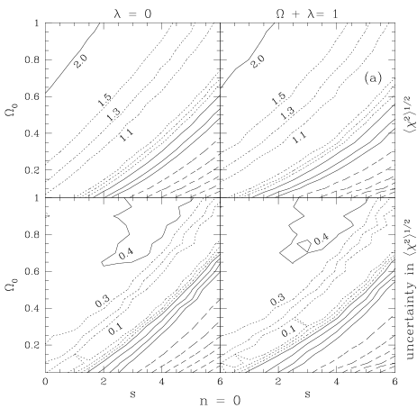
Figure 8: The square root of the reduced chi-squared parameter for all models is displayed, as well as the “uncertainty” in this parameter, the derivation of which is described in the text. In the upper row, dotted-line contours have been drawn corresponding to $\langle\chi^{2}\rangle^{1/2}$ = 1.07, 1.28, and 1.51, which represent formal probabilities of about 30%, 5%, and 0.3% that the data come from the same underlying distribution as the model and differ only through gaussian random variations. Solid-line contours have been drawn at $\langle\chi^{2}\rangle^{1/2}$ = 2.0, 3.0, and 4.0, which correspond to very small probabilities but may be useful in combination with the uncertainties. The dashed lines are drawn every time the likelihood parameter doubles thereafter, i.e. at levels of 8.0, 16.0, etc. In the lower row, the dotted-line contours are drawn at uncertainty levels of 0.1, 0.2, and 0.3; the solid lines at levels of 0.4, 0.6, 0.8, and 1.0, and the dashed lines at each doubling over 1.0. Note that although the uncertainties get very high in the region of low $\Omega_{0}$ and high $s$, the likelihood parameter is larger still by about a factor of 4. Figure (8a) displays models with $n\!=\!0$, Figure (8b) with $n\!=\!-1$ and Figure (8c) with $n\!=\!-2$.

Changing the cosmological parameters over the proposed range can produce massive overabundances or moderate underabundances. To assess the likelihood of each model we compare the predicted differential logN–logS (the number of clusters in a specified flux bin) to the data points and calculate the reduced chi-squared factor for that model. The full set of data used to constrain our parameter space includes the faintest 6 data points from the WARPS sample and ten points from Rosati’s, for sixteen degrees of freedom altogether. The use of differential data means that statistical errors are formally independent. We employ a chi-squared statistic because it provides a measure of the absolute goodness of fit for the models, assuming the error bars are Gaussian. Our results would be similar were we to employ a maximum likelihood approach. The main disadvantage of this approach is the difficulty in including the uncertainty in $L_{15}$ and $p$ for a particular model. We adopt an approximate procedure to solve this problem, which will be described shortly.

Figures 8(a-c) present the “likelihood” plots of all models having $n=0$, $-1$ and $-2$, respectively. The value displayed in the upper row for each model is the square root of the reduced chi-squared parameter $\langle\chi^{2}\rangle^{1/2}$, where the average is over all data points in the logN–logS. The dotted contours in the upper row mark models which deviate from the data at one, two, and three-sigma confidence levels. The main limitation in the ability of theory to predict abundances accurately at this level of analysis is the determination of $L_{15}$ and $p$. Although an accuracy of 5% to 10% is quite good (and quite possibly as good as we’re going to get, since this method is limited by the number of nearby clusters), varying these numbers within their confidence limits can still produce considerable changes in the predicted logN–logS (see Figure 4).

To account for this, we calculated the likelihood parameter, $\langle\chi^{2}\rangle^{1/2}$, for the four vertices of the standard error ellipse in $L_{15}$–$p$ space as well as for the best-fit model. The uncertainty shown is the difference in $\langle\chi^{2}\rangle^{1/2}$ between the best-fit case and the perturbed case which gave the smallest value of the likelihood parameter. The results are presented in the lower rows of Figures 8(a-c) and can be interpreted as a “one-sigma” uncertainty in the contours of the top row. Keep in mind that this variance is not symmetric; we present only the difference in the direction of greater likelihood. Since our aim here is to provide a reasonable indication of the uncertainty in the modeling, this heuristic error estimate seems sufficient. The data were presented in this manner to make it possible for the reader to estimate constraints at other confidence levels.

It is clear from Figures 8(a-c) that the results are not strongly affected by the value of $\lambda_{0}$. Introducing a cosmological constant increases the volume element per redshift bin throughout most of the integration range, which reduces the observed flux of each cluster, but it also increases the total surface density of clusters. As can be seen from a close examination of the figures, in most regions of the parameter space introducing a cosmological constant slightly raises the value of $\Omega_{0}$ required for a good fit. Since raising $\Omega_{0}$ lowers the number of clusters, we conclude that increased integration volume is the dominant effect for most models. In other words, setting $\lambda_{0}\neq 0$ tends to increase the surface density of clusters, and a higher value of $\Omega_{0}$ is needed to compensate.

Changing the spectral index $n$ has a quite strong effect on the derived mass-luminosity relationship (Figure 2), which as we will see can have important consequences. Because all of the models are constrained to agree with local abundances, however, $n$ has limited leverage on the distant cluster population. The main effect on the logN–logS is that models with larger $n$ have sharper exponential cutoffs in their mass distribution, resulting in a lower cluster surface density. The best-fitting models for $n\!=\!0$ thus have lower $\Omega_{0}$ and greater luminosity evolution to compensate.

The clearest relationship visible in Figures 8(a-c) is, of course, that between the density and evolution parameters, $\Omega_{0}$ and $s$. It seems from these results that if we wish to believe in the degree of evolution indicated by self–similar or constant entropy arguments — $s\!=\!3.5$ and $11/4$, respectively — then we obtain a useful lower bound of $\Omega_{0}\mathrel{\hbox to0.0pt{\lower 3.0pt\hbox{$\mathchar 536\relax$}\hss}\raise 2.0pt\hbox{$\mathchar 318\relax$}}0.3$. The lower end of this range is consistent with limits from the mean intracluster gas fraction of clusters, which give $\Omega_{0}h^{2/3}\!=\!0.28\pm 0.07$ (Evrard 1997) in the most straightforward interpretation.

Conversely, if the degree of luminosity evolution is instead very small — $s\mathrel{\hbox to0.0pt{\lower 3.0pt\hbox{$\mathchar 536\relax$}\hss}\raise 2.0pt\hbox{$\mathchar 316\relax$}}1$ — then the analysis strongly rules out a critical density universe. Recall that all the off-ridge models which have $\Omega_{0}\!=\!1$ underpredict the number of observed clusters (see Figures 5-7), and these should be treated more harshly given the possibility for survey incompleteness. It seems that if the universe does indeed have a critical density, we need at least a moderate degree of evolution in the cluster luminosity to fit the data well. The assumption of constant cluster entropy ($s=11/4$) put forward in EH91 would be sufficient to allow such models. The preferred region, however, indicates an even larger degree of evolution. This could come about if radiative cooling occurs on a much longer time scale than gravitational collapse (Bower 1997), or if a significant amount of energy is injected into the ICM by galaxies (e.g., Metzler & Evrard 1994).

	$\lambda_{0}=0$			$\Omega_{0}+\lambda_{0}=1$
Constraint	$n=0$	$n=-1$	$n=-2$	$n=0$	$n=-1$	$n=-2$
$\Omega_{0}=1.0$	$s\geq 3.5$	$s>3.0$	$s>2.5$	$s\geq 3.5$	$s>3.0$	$s>2.5$
$s=3.5$	$\Omega_{0}>0.20$	$\Omega_{0}>0.25$	$\Omega_{0}>0.35$	$\Omega_{0}>0.20$	$\Omega_{0}>0.25$	$\Omega_{0}>0.35$
$s=1.0$	$\Omega_{0}\leq 0.45$	$\Omega_{0}<0.60$	$\Omega_{0}\leq 0.75$	$\Omega_{0}\leq 0.45$	$\Omega_{0}<0.65$	$\Omega_{0}<0.80$
$s=0.0$	$\Omega_{0}<0.30$	$\Omega_{0}\leq 0.40$	$\Omega_{0}\leq 0.60$	$\Omega_{0}<0.35$	$\Omega_{0}\leq 0.45$	$\Omega_{0}\leq 0.65$

Table 1: A summary of the constraints that can be placed on $\Omega_{0}$ and $s$ using the information in Figures 8. All of these constraints are at the 95% confidence level, after accounting for the displayed uncertainty in the chi-squared parameter.

The results of this analysis are summed up in Table 1. The limits put down are at the 95% (about 2 $\sigma$) confidence level (i. e. there is only a 5% chance of the model randomly producing the observed data), after reducing the $\langle\chi^{2}\rangle^{1/2}$ parameter by the uncertainty indicated in Figures 8(a-c). The models are examined in intervals of 0.05 in $\Omega_{0}$ and 0.5 in $s$, so a $\geq$ or $\leq$ sign just means that the limiting model was at or very near the required confidence level of 95%. In addition, all of the disallowed models indicated here underpredicted the number of clusters, except for those which assumed $s\!=\!3.5$. The constraints thus allow for a one-sigma variation in $L_{15}$ and $p$ tailored to bring the model closer to the data, and can be treated as conservative conclusions.

4 Additional Constraints from the Cluster Population

4.1 The Luminosity-Temperature Relation

Because of the degeneracy between intrinsic luminosity evolution and cosmological evolution, the logN–logS alone limits models to the ridge seen in Figure 8. It is worthwhile to see what additional constraints can be placed on the parameter space by including additional observational information. One interesting question is what each model predicts for the X–ray luminosity—temperature correlation. So far, we have made use of the virial relationship $T\propto M^{2/3}$ only to tabulate the band fraction. Because the fraction $f_{E}(T)$ for the ROSAT bands is a weakly dependent function of temperature, our results up to this point would change very little if we were to adopt a different $T(M)$ behavior. If we are willing to promote virial equilibrium to a strong assumption, however, we can use it as an independent test of the parameter $p$. There is good theoretical support from numerical simulations for virial equilibrium within the non–linear portions of clusters (Evrard et al.1996) and modest empirical support for this assumption from analysis of the mean intracluster gas fraction (Evrard 1997). Comparison with the values derived from the BCS XLF fit then provides an added, non–trivial constraint on the models.

The virial scaling assumption $T\propto M^{2/3}(1+z)$ translates directly into a bolometric $L_{X}$–$T$ relation of the form

$$L_{X}\ \propto\ T^{3p/2}(1+z)^{s-3p/2}$$ (14)

The observed relationship is, roughly, $L_{X}\propto T^{2.8\pm 0.3}$. (Edge & Stewart 1991; Arnaud 1994). The quoted error in the slope is more generous than those reported in individual works, in order to allow for possible systematic uncertainties betwen different data sets. Consistency with the observed slope requires $p=1.9\pm 0.2$. This range, drawn in Figure 2 as dotted horizontal lines, incorporates the value $11/6$ appropriate for the constant central entropy model of EH91 (see also Bower 1997). A quick glance at the figure reveals that including this result puts a strong constraint on $\Omega_{0}$ and $n$. If $n=-1$, this range of values is found only in very low-density universes ($\Omega_{0}\mathrel{\hbox{\hbox to0.0pt{\hbox{\lower 4.0pt\hbox{$\sim$}}\hss}\hbox{$<$}}}0.1$). For models with $n=-2$, on the other hand, we find acceptable values of $p$ in the range $0.25\leq\Omega_{0}\leq 1.0$. If a cosmological constant is included, the allowed range in $\Omega_{0}$ shifts to slightly higher values.

The real perturbation spectrum is not likely a pure power law, but this analysis indicates models with effective spectral index $n\mathrel{\hbox{\hbox to0.0pt{\hbox{\lower 4.0pt\hbox{$\sim$}}\hss}\hbox{$<$}}}-1.5$ are favored in universes with reasonable values of the density parameter. Such “red” spectral values are also favored by the shape of the temperature abundance function (Henry & Arnaud 1991; Oukbir, Bartlett & Blanchard 1997). For reference, Huss, Jain & Steinmetz (1997) present a list of effective spectral indices ($n_{eff}\!\equiv\!\hbox{\rm d$\,$ln }P(k)/\hbox{\rm d$\,$ln }k$) for a number of popular cosmological models. A cold, dark matter model with $\Omega_{0}\!=\!0.3$, $\Lambda\!=\!0$ and $h\!=\!0.7$ has $n_{eff}\!=\!-1.74$, for example.

Room to maneuver around this conclusion can be gained by invoking a degree of scatter in the relationship between bolometric X-ray luminosity and binding mass. Scatter will tend to flatten the slope and increase abundance at the bright end of the predicted luminosity function, implying a bias toward overestimating $p$ and $L_{15}$ compared to the case with no scatter. The amount of scatter is not known a priori, but a likely lower bound can be obtained from gas dynamic simulations. The two sets of 18 cluster simulations of Metzler (1995) revealed a scatter of magnitude $\langle\delta(\log L_{X})^{2}\rangle=0.047$ for simulations involving dark matter and baryon fluids, and $\langle\delta(\log L_{X})^{2}\rangle=0.026$ for simulations which also included a model for the ejection of gas from galaxies into the ICM. We have checked that including scatter at the larger of the above values results in a fractional change in the best fit $p$ of at most $10\%$, comparable to the uncertainty from the BCS XLF fit. We conclude that such modest levels of scatter are not strongly affecting our results. Larger amounts of scatter would lead to downward revisions in our best fit values of $p$ in Figure 2, and so would somewhat relax constraints on the effective spectral index on cluster scales.

Another important prediction from equation (14) is that we expect redshift evolution in the bolometric luminosity at a fixed temperature proportional to $(1+z)^{s-3p/2}$. Since fitting the local relation requires $3p/2\!=\!2.8\pm 0.3$, the expectation is of an offset in the intercept of the $L_{X}-T$ relation of amplitude

$$\Delta(\log L_{X}(z))\,{|}_{T}\ =\ [s-(2.8\pm 0.3)]\,\Delta(\log(1+z))$$ (15)

independent of spectral index or cosmology. Both the original self–similar value $s\!=\!7/2$ and the constant central entropy value $s=11/4$ predict very little change in the intercept of the $L_{X}$–$T$ relation back to $z\!\simeq\!0.5$. The full range we investigate, $s\in[0,6]$, translates into shifts of factors ranging from about one–third to three at $z=0.5$.

Comparing a recent compilation of 15 distant clusters ($\langle z\rangle\simeq 0.33$) by Henry et al.(1997) with a similar sample of the nearby population ($\langle z\rangle\simeq 0.07$) by David et al.(1993) provides us with an early estimate of this shift. Comparing the intercepts of the two samples, we find $\Delta(\log L_{X})/\Delta(\log(1+z))\!=\!1.1\pm 1.1$ at the one-sigma level, which corresponds to a plausible range of $2.5\leq s\leq 5.3$. The observations rule out very low values of the evolutionary parameter $s$, and therefore eliminate the low $\Omega_{0}$ end of the allowed ridge in Figure 8.

4.2 Redshift Distributions

Figure 9: The cumulative and differential redshift distributions for the $\lambda\!=\!0$, $n\!=\!-2$ models described in the text. The effect of changing $\Omega_{0}$ and $s$ can be clearly seen here; increasing $\Omega_{0}$ sharply reduces the number of high-redshift clusters, while increasing $s$ brings the lower-mass objects above the flux limit.

Additional constraints can be found by examining the redshift distribution of the clusters, which can be expected to vary strongly with our choice of cosmology. Indeed, Oukbir & Blanchard (1997), employing methods similar to ours, found the redshift distribution in the EMSS sample (Gioia & Luppino 1994) to be well fit by either a low density model with mild evolution ($\Omega_{0}\!=\!0.2$, $s\!=\!0.5$ in our terminology) or an Einstein–deSitter model with more rapid evoluition ($\Omega_{0}\!=\!1$, $s\!=\!3.8$). These models lie along the ridge allowed by the ROSAT counts in our analysis.

As discussed in section 3.1, the redshift distribution is straightforward to calculate for a given model and flux limit. Although obtaining accurate redshifts for clusters is a time-consuming process, the shape of this statistic is not strongly dependent on small differences in the efficiency of flux reconstruction or the choice of model for cluster surface brightness. A confident flux limit and a well-understood sky coverage function, are, however, necessary to predict the normalization of these curves.

Figure 9 displays the differential and cumulative distributions at a flux limit of $5.5\times 10^{-14}$ erg sec^-1 cm^-2 in the band 0.5-2.0 keV, the parameters of the WARPS survey. Each category of models is represented by four specific choices within the region of plausible likelihood, all of which assume $n\!=\!-2$:

1. $\Omega_{0}=0.3$, $s=1.0$

2. $\Omega_{0}=0.3$, $s=2.75$

3. $\Omega_{0}=1.0$, $s=2.75$

4. $\Omega_{0}=1.0$, $s=6.0$

Models (i) and (iv) fit all of the logN–logS data quite well, lying near the center of the ridge described by Figure 8c, but model (i) predicts a decrease in the zero–point of the $L_{x}$–$T$ relation larger than observed. Models (ii) and (iii) are given as reference points, and to display the effects of moving perpendicular to the ridge in the $\Omega_{0}$–$s$ plane. These models are ruled out at about the 95% confidence level after subtracting the uncertainty in their likelihood parameters, but make the effect of changing the parameters clearer.

As you can see, the redshift distribution does not discriminate well between models which lie on the ridge in Figure 8c, but displays significant differences when the parameters are changed in other directions. Samples of size approaching 100 clusters are soon arriving (Rosati 1997, private communication) and these will provide stringent tests of the models by constraining the area under the high redshift tail of the distribution. In particular, if $\Omega_{0}\simeq 0.3$ as indicated by the mean intracluster gas fraction and $s$ is close to the $11/4$ fixed core entropy value (model ii), then we predict 10% of clusters above the WARPS survey flux limit should lie at $z\geq 0.75$.

5 Conclusions and Future Directions

We assume that the underlying number density of clusters as a function of mass is well described by the Press-Schechter function and model the scaling of cluster bolometric luminosity and temperature as power–laws in binding mass and epoch. For a given cosmological model, we determine the free parameters of the current mass-luminosity relation by fitting the predicted X–ray luminosity function to the BCS XLF (Ebeling et al. 1996), and integrate the abundance function out to high redshifts to compute counts.

A direct comparison by means of chi-squared analysis made to differential logN–logS data from two ROSAT surveys produces a ridge of acceptable models following roughly $s\simeq 6\Omega_{0}$. If $s$ is in fact about equal to 3 as expected from simple theoretical arguments (Kaiser 1986, EH91) then the universe seems to require at least a moderate density parameter $\Omega_{0}\mathrel{\hbox to0.0pt{\lower 3.0pt\hbox{$\mathchar 536\relax$}\hss}\raise 2.0pt\hbox{$\mathchar 318\relax$}}0.3$ in order to bring the cluster number counts down to observed levels. Conversely, a universe with critical density is inconsistent with a low evolution parameter $s\mathrel{\hbox to0.0pt{\lower 3.0pt\hbox{$\mathchar 536\relax$}\hss}\raise 2.0pt\hbox{$\mathchar 316\relax$}}2.5$; such models are strongly ruled out because they underpredict the number of clusters and are harder to save by invoking systematic errors in the surveys. Although changing the slope of the power spectrum and incorporating a cosmological constant also affected these results, these parameters contribute only slightly to the overall behaviour. An independent constraint from the local, observed $L_{X}$–$T$ relation limits singles out the $n\!=\!-2$ plane, further reducing the space of allowed models.

The logN–logS alone is a useful, but limited, discriminator of cosmological models. Because the local XLF is used to determine the mass-luminosity relationship, the predicted counts will always be limited in accuracy by the level of shot noise in the local cluster population. Assuming that the local XLF will not increase much in accuracy, this method has the potential to pin down a region in the $\Omega_{0}$-$s$ plane with a width of about $\pm 0.1$ in $\Omega_{0}$ and $\pm 1.0$ in $s$. This estimate was made under the assumption that the uncertainties arising from the XLF are the only significant ones; in practice this level of discriminating power could be achieved when the overall uncertainties on the logN–logS data have decreased to about one-third their current size.

One could try to improve the accuracy of this method by pushing observations down to a lower flux limit, but the returns are limited by the local XLF uncertainty. In order for a new data point at a fainter flux limit to be useful, it needs to have error bars significantly smaller than the uncertainty in the logN–logS from the local XLF. For example, the uncertainty on the integrated logN–logS at a flux limit of $10^{-15}\hbox{$\,$ erg s${}^{-1}$}$ is about 30%. We estimate that a data point with 10% error bars would make a useful contribution to the discriminating power of this method. Assuming simple Poisson errors, this level of precision could be achieved with a sample of about 100 clusters, over 1-2 square degrees of sky. Toy models show that such a point would strengthen the lower limit on $s$ for critical density universes, and greatly increase the lower limits on $\Omega_{0}$ for models with moderate $s$.

Independent observations can be used to narrow the allowed range in parameter space. Assuming clusters are in virial equilibrium, the shift in the zero–point of the $L_{x}$–$T$ relation limits the evolutionary parameter $s$. Current observations at $\langle z\rangle\sim 0.3$ (Henry et al.1997; Mushotzky & Scharf 1997) indicate $s$ lies in the range $2.5$ to $5$. Similar data at higher redshifts, with subsequently longer lever arm in equation (15), would be very useful in reducing the allowed range. Redshift distributions of X–ray flux limited samples provide additional independent constraints (Oukbir & Blanchard 1997; Bower 1997). The extent of the high redshift tail of the distribution is a sensitive indicator of which side of the $\Omega_{0}$–$s$ ridge the universe lies. If $\Omega_{0}\simeq 0.3$ as indicated by the mean intracluster gas fraction (Evrard 1997) and $s\geq 11/4$, then we predict at least 10% of clusters above the WARPS survey flux limit should lie at redshifts $z\geq 0.75$.

Appendix A Calculating $\delta_{c}(z)$

The critical overdensity $\delta_{c}(z)$ is defined as the linearly extrapolated overdensity of a perturbation that has just collapsed at redshift $z$. For universes with $\Omega_{0}=1$, this number is the canonical $\delta_{c}=1.686$; for open universes or flat universes with $\lambda_{0}\neq 0$ this overdensity will be somewhat smaller. Since the CDM power spectrum used in our analysis is normalized to the COBE microwave background measurements and therefore the power spectrum at the present day, the critical overdensity of a perturbation collapsing at redshift $z$ is further extrapolated to a redshift of zero using the linear growth factor appropriate to the cosmology. This quantity is labeled $\delta_{c0}(z)$. All the following relations are derived using the spherical collapse model.

For a flat universe with $\Omega_{0}=1$, we use the following relations

$$\delta_{c}(z) = \frac{3}{20}(12\pi)^{2/3}$$ (16)

$$\delta_{c0}(z) = (1+z)\delta_{c}(z)$$ (17)

For an open universe with $\Omega_{0}<1$ and $\lambda_{0}=0$ we use the relationship derived by Cole and Lacey (1993)

$$\delta_{c}(z) = \frac{3}{2}D(z)\left(1+\frac{2\pi}{\sinh(\eta)-\eta}\right)^{2/3}$$ (18)

$$\delta_{c0}(z) = \frac{D(0)}{D(z)}\delta_{c}(z)$$ (19)

$$D(0) = 1+\frac{3}{x_{0}}+\frac{3\sqrt{1+x_{0}}}{x_{0}^{3/2}}\ln(\sqrt{1+x_{0}}-\sqrt{x_{0}})$$ (20)

where $x_{0}\equiv\Omega_{0}^{-1}-1$, $\eta\equiv\cosh^{-1}(2/\Omega(z)-1)$, and $D$ represents the linear growth factor.

Finally, for a flat universe with $\Omega_{0}+\lambda_{0}=1$ we use an approximate parameterization to the Eke et al. (1996) results for $\delta_{c}(z)$

$$\delta_{c}(z)=1.68660[1+0.01256\log\Omega(z)]$$ (21)

The form of the parameterization was inspired by Kitayama and Suto (1997). This reference also contains the functional form of the exact solution, which is a hypergeometric function of type (2,1). To get $\delta_{c0}(z)$ for this type of universe we use the solution for the linear growth factor found in Peebles (1980), §13

$$D_{1}(x)=\frac{\sqrt{(x^{3}+2)}}{x^{3/2}}\int_{0}^{x}x^{3/2}_{1}(x_{1}^{3}+2)^{-3/2}dx_{1}$$ (22)

where $x=a/a_{e}$, and $a_{e}=[(1-\lambda_{0})/(2\lambda_{0})]^{1/3}$, the inflection point in the scale factor. In our analysis this function is integrated numerically to find the growth factor at redshifts $z$ and 0, and then $\delta_{c0}(z)$ again equals $\delta_{c}(z)D(0)/D(z)$.

Appendix B The Volume Element for $\lambda_{0}\neq 0$

The number of clusters in a given volume element dV centered at redshift $z$ and mass range dM is given by the Press-Schechter abundance times the differential volume

$$dN(M)=n(M,z)dVdM=n(M,z)\frac{r^{2}drd\Omega}{\sqrt{1-kr^{2}}}dM$$ (23)

To integrate this function over a range in redshift rather than in physical distance, we need to find $r(z)$ for a particular cosmology and make the transformation to the form

$$dN(M)=n(M,z)f(z)dz\,d\Omega\,dM$$ (24)

For a universe with $\Omega_{0}+\lambda_{0}=1$, $k=0$ and $f(z)=r^{2}dr/dz$. The function $r(z)$ can be tabulated by integrating along the null geodesic:

$$r=\int_{0}^{r}dr^{\prime}=\int_{a}^{a_{0}}\frac{da}{\dot{a}a}$$ (25)

We can then express the Friedmann equation in terms of today’s values of the cosmological parameters

$$\dot{a}=aH_{0}\sqrt{\frac{\Omega_{0}}{a^{3}}+\lambda_{0}}$$ (26)

and insert this into the geodesic integral to get $r(z)$ in a straightforward manner. The integral obtained has an exact solution in terms of elliptic integrals of the first kind, but expressing it in this manner requires the integral to be performed from $a=0$. In addition, for $\lambda_{0}$ greater than about 0.7, the elliptic integral must be evaluated outside of its defined domain. It is computationally more reliable to evaluate the integral numerically. For those who are interested, the “exact” solution is

$$\frac{r(z)}{r_{0}} = \ \ F\left(\cos^{-1}\left[\frac{1+(1-\sqrt{3})u_{0}}{1+(1+\sqrt{3})u_{0}}\right],\kappa\right)$$

$$\!\!\mbox{}-F\left(\cos^{-1}\left[\frac{1+(1-\sqrt{3})u_{z}}{1+(1+\sqrt{3})u_{z}}\right],\kappa\right)$$

where $u_{0}=(\lambda_{0}/\Omega_{0})^{1/3}$, $u_{z}=u_{0}/(1+z)$, $\kappa=\sqrt{2+\sqrt{3}}/2$, and $r_{0}=c/(H_{0}\Omega_{0}^{1/3}\lambda_{0}^{1/6}\sqrt[4]{3})$.

References

- [1] Arnaud, M. 1994, in Cosmological Aspects of X–ray Clusters of Galaxies, ed., W.C. Seiter, NATO ASI Series C, 441, 197.
- [2] Bower R. G. 1997, MNRAS, in press
- [3] Castander F. J. et al., 1995, Nat, 377, 39
- [4] Collins C. A., Burke D. J., Romer A. K., Sharples R. M., Nichol R. C., ApJL, submitted 10/96
- [5] David L. P., Slyz A., Jones C., Forman W., Vrtilek S. D., Arnaud K. A., 1993, ApJ, 412, 479
- [6] Ebeling H., 1993, Abell and ACO Clusters of Galaxies in the ROSAT All-Sky Survey: a Statistical Study, PhD thesis, MPE report 250
- [7] Ebeling H., Wiedenmann G., 1993, Phys. Rev. E, 47, 704
- [8] Ebeling H., Allen S. W., Crawford C. S., Edge A. C., Fabian A. C., Böhringer H., Voges W., Huchra J. P., 1995, Conference Proceedings of Röntgenstrahlung from the Universe, Würzburg
- [9] Ebeling H., Edge A. C., Fabian A. C., Allen S. W., Crawford C. S., Böringer H., 1997, ApJ Letters, April 20
- [10] Edge A. C., Stewart G. C., 1991, MNRAS, 252, 428
- [11] Eke V. R., Cole S., Frenk C. S., 1996, MNRAS, 282, 263
- [12] Evrard A. E., 1990a, ApJ, 363, 349
- [13] Evrard A. E., 1990b, in Oegerle W. R., Fitchett M. J., Danly L., eds, Clusters of Galaxies, Cambridge Univ. Press, Cambridge, 287
- [14] Evrard A. E. 1997, MNRAS, submitted (astro-ph/9701148)
- [15] Evrard A. E., Henry J. P., 1991, ApJ, 383, 95
- [16] Evrard A. E., Metzler C., Navarro, 1996, ApJ, 469, 494
- [17] Gioia I. M., Henry J. P., Maccacaro T., Morris S. L., Stocke J. T., Wolter A., 1990a, ApJ, 356, L35
- [18] Gioia I. M., Maccacaro T., Schild R. E., Wolter A., Stocke J. T., Morris S. L., Henry J. P., 1990b, ApJ Supplement Series, 72, 567
- [19] Henry J.P., Arnaud, K.A. 1991, ApJ, 372, 410
- [20] Henry J. P., Gioia I. M., Maccacaro T., Morris S. L., Stocke J. T., Wolter A., 1992, ApJ, 386, 408
- [21] Huss, A., Jain, B., Steinmetz, M. 1997, (astro-ph/9703014)
- [22] Jones L. R., Scharf C., Perlman E., Ebeling H., Wegner G., Malkan M., 1997, in preparation.
- [23] Kaiser N., 1986, MNRAS, 222, 323
- [24] Kaiser N., 1991, ApJ, 383, 104
- [25] Kitayama T., Suto Y., 1997, ApJ, in press
- [26] Lacey C., Cole S., 1993, MNRAS, 262, 627
- [27] Luppino G. A., Gioia I. M., 1995, ApJ, 445, L77
- [28] Metzler C., PhD thesis, University of Michigan
- [29] Mushotzky, R.F., Scharf, C.A. 1997 (astro-ph/9703039)
- [30] Nichol R. C., Holden B. P., Romer A. K., Ulmer M. P., Burke D. J., Collins C. A., 1997, ApJ, in press
- [31] Oukbir J., Blanchard A., 1997, A & A, in press
- [32] Oukbir J., Bartlett J. G., Blanchard A., 1997, A & A, in press
- [33] Peebles, P. J. E., 1980, The Large Scale Structure of the Universe, Princeton University Press, Princeton, 1980
- [34] Press W. H., Schechter P., 1974, ApJ, 187, 425
- [35] Richstone D., Loeb A., Turner E. L., 1992, ApJ, 393, 477
- [36] Rosati P., 1995c, PhD thesis, University of Rome
- [37] Rosati P., Della Ceca R., 1995b, Conference Proceedings of Röntgenstrahlung from the Universe, Würzburg
- [38] Rosati P. & Della Ceca R., 1997, in preparation
- [39] Rosati P., Della Ceca R., Burg R., Norman C., Giacconi R., 1995a, ApJ, 445, L11.
- [40] Scharf C., Jones L. R., Ebeling H., Perlman E., Malkan M., & Wegner G., 1997, ApJ, in press.
- [41] White, S.D.M., Efstathiou, G., Frenk, C.S. 1993, MNRAS 262, 1023.
- [42] Viana P. T. P., Liddle A. R., 1996, MNRAS, 281, 323
- [43] Vikhlinin A., Forman W., Jones C., McNamara B., 1996, BAAS, 188, #06.10