The Lyman Alpha Forest Within The Cosmic Web

Abstract

Observations indicate galaxies are distributed in a filament-dominated web-like structure; classic examples are the Coma and Perseus-Pisces superclusters. Numerical experiments at high and low redshift of viable structure formation theories also show filament-dominance; in particular, the gasdynamical simulations of Ly$\alpha$ clouds at redshifts $\sim 2-6$ that we concentrate on here. We understand why this is so in terms of rare events (peak patches) in the medium and the web pattern of filaments that bridge the gaps between the peaks along directions defined by their (oriented) tidal fields. We present an overview of these ideas and their practical application in crafting high resolution well-designed simulations. We show the utility of this by taking a highly filamentary subvolume found in a galactic-scale simulation, compressing its important large scale features onto a handful of numbers defining galactic-scale peak-patch constraints, which are then used to construct constrained initial conditions for a higher resolution simulation appropriate for study of the Ly$\alpha$ forest.

1 The Peak Patch Picture and the Cosmic Web Theory of Filaments

We approach the connected ideas we loosely call Cosmic Web theory (Bond, Kofman and Pogosyan 1996, BKP) and the Peak Patch Picture (Bond and Myers 1996, BM, refer here for pre-1995 work) through a historical path that includes an outline of the relevant terminology. In 1965, Lin, Mestel & Shu showed that a cold triaxial collapse implied an oblate “pancake” would form. In 1970, Zeldovich developed his famous approximation and argued that pancakes would be the first structures that would form in the adiabatic baryon-dominated universes popular at that time. Generally for a cold medium, there is a full non-linear map: ${\bf x}({\bf r},t)\equiv{\bf r}-{\bf s}({\bf r},t)$, from Lagrangian (initial state) space, ${\bf r}$, to Eulerian (final state) space, ${\bf x}$. The map becomes multivalued as nonlinearity develops in the medium. It is conceptually useful to split the displacement field, ${\bf s}={\bf s}_{b}+{\bf s}_{f}$, into a smooth quasilinear long wavelength piece ${\bf s}_{b}$ and a residual highly nonlinear fluctuating field ${\bf s}_{f}$. If the rms density fluctuations smoothed on scale $R_{b}$, $\sigma_{\rho}(R_{b})$, are $<{\cal O}(1/2)$, the ${\bf s}_{b}$-map is one-to-one (single-stream) except at the rarest high density spots. In the peak patch approach, $R_{b}$ is adaptive, allowing for dynamically hot regions like protoclusters to have large smoothing and cool regions like voids to have small smoothing. If $D(t)$ is the linear growth factor, then ${\bf s}_{b}=D(t){\bf s}_{b}({\bf r},0)$ describes Lagrangian linear perturbation theory, i.e. the Zeldovich approximation. The large scale peculiar velocity is ${\bf V}_{Pb}=-\bar{a}(t)\dot{{\bf s}}_{b}({\bf r},t)$. What is important for us is the strain field (or deformation tensor):

$$e_{b,ij}({\bf r})\equiv-{1\over 2}\big{(}{\partial s_{bi}\over\partial r_{j}}+{\partial s_{bj}\over\partial r_{i}}\big{)}({\bf r})=-\sum_{A=1}^{3}\lambda_{vA}{\hat{n}}_{vA}^{i}{\hat{n}}_{vA}^{j},{\rm~{}where}$$

$$\ \lambda_{v3}={\delta_{Lb}\over 3}(1+3e_{v}+p_{v}),\ \lambda_{v2}={\delta_{Lb}\over 3}(1-2p_{v}),\ \lambda_{v1}={\delta_{Lb}\over 3}(1+3e_{v}-p_{v}),$$

and $\delta_{Lb}=-e_{b,i}^{i}$ is the smoothed linear overdensity, which we often express in terms of the height relative to the rms fluctuation level $\sigma_{\rho}(R_{b})$, $\nu_{b}\equiv\delta_{Lb}/\sigma_{\rho}(R_{b})$. The deformation eigenvalues are ordered according to $\lambda_{v3}\geq\lambda_{v2}\geq\lambda_{v1}$ and ${\hat{n}}_{vA}$ denote the unit vectors of the principal axes. In that system, $x_{A}=r_{A}(1-\lambda_{vA}({\bf r},t))$ describes the local evolution. The Zeldovich-mapped overdensity is $(1+\delta_{Z})({\bf r},t)=|{(1-D(t)\lambda_{v3})(1-D(t)\lambda_{v2})(1-D(t)\lambda_{v1})}|^{-1}$, exploding when the largest eigenvalue $D(t)\lambda_{v3}$ reaches unity (fold caustic formation). In a Zeldovich map a pancake developes along the surface ${\hat{n}}_{v3}\cdot\nabla_{{\bf r}}\lambda_{v3}=0$.

The strain tensor is related to the peculiar linear tidal tensor by ${\partial^{2}\Phi_{P}\over\partial x^{i}\partial x^{j}}=-4\pi G{\bar{\rho}}_{nr}\bar{a}^{2}\,e_{b,ij}$, where $\Phi_{P}$ = peculiar gravitational potential, and to the linear shear tensor by ${\dot{e}}_{b,ij}$. The anisotropic part of the shear tensor has two independent parameters, the ellipticity $e_{v}$ (always positive) and the prolaticity $p_{v}$.

Doroshkevich (1973) and later Doroshkevich & Shandarin (1978) were among the first to apply the statistics of Gaussian random fields to cosmology, in particular of $\lambda_{vA}$, at random points in the medium. Arnold, Shandarin and Zeldovich (1982) made the important step of applying the catastrophe theory of caustics to structure formation. This work suggested the following formation sequence: pancakes first, followed by filaments and then clusters. This should be compared to the BKP Web picture formation sequence: clusters first, followed by filaments and then walls. BKP also showed that filaments are really ribbons, walls are webbing between filaments in cluster complexes, and that walls are not really classical pancakes. For the Universe at $z\sim 3$, massive galaxies play the role of clusters, and for the Universe at $z\sim 5$ more modest dwarf galaxies take on that role.

The Web story relies heavily upon the theory of Gaussian random fields as applied to the rare “events” in the medium, e.g., high density peaks. Salient steps in this development begin with Bardeen et al. (1986, BBKS), where the statistics of peaks were applied to clusters and galaxies, e.g., the calculation of the peak-peak correlation function, $\xi_{pk,pk}$. In a series of papers, Bond (1986-90) and Bond & Myers (1990-93) developed the theory so that it could calculate the mass function, $n(M)dM$. It was also applied to the study of how shear affects cluster alignments (e.g., the Binggeli effect), and to Ly$\alpha$ clouds, ‘Great Attractors’, giant ‘cluster-patches’, galaxy, group and cluster distributions, dusty PGs, CMB maps and quasars. This culminated in the BM “Peak-Patch Picture of Cosmic Catalogues”.

We briefly describe the BM peak patch method and how it is applied to initial conditions for simulations; an example is shown in Fig. 1. We identify candidate peak points using a hierarchy of smoothing operations on the linear density field $\delta_{L}$. To determine patch size and mass we use an ellipsoid model for the internal patch dynamics, which are very sensitive to the external tidal field. A byproduct is the internal (binding) energy of the patch and the orientation of the principal axes of the tidal tensor. We apply an exclusion algorithm to prevent peak-patch overlap. For the external dynamics of the patch, we use a Zeldovich-map with a locally adaptive filter ($R_{pk}$) to find the velocity ${\bf V}_{pk}$ (with quadratic corrections sometimes needed). The peaks are rank-ordered by mass (or internal energy). Thus, for any given region, we have a list of the most important peaks. By using the negative of the density field, we can also get void-patches. Some of the virtues of the method are: it represents a natural generalization of the Press-Schechter method to include non-local effects; is a natural generalization of BBKS single-filter peaks theory to allow a mass spectrum and solve the cloud-in-cloud (i.e., peak-in-peak) problem; allows efficient Monte Carlo constructions of 3D catalogues; gives very good agreement with $N$-body groups; has an accurate analytic theory with which to estimate peak properties, (e.g., mass and binding energy from mean-profiles, using $\delta_{L,crit}(e_{v})$, $\langle{e_{v}|\nu_{pk}\rangle}$); and handles merging, with high redshift peaks being absorbed into low redshift ones.

BKP concentrated on the impact the peak-patches would have on their environment and how this can be used to understand the web. They showed that the final-state filament-dominated web is present in the initial conditions in the $\delta_{Lb}$ pattern, a pattern largely determined by the position and primordial tidal fields of rare events. BKP also showed how 2-point rare-event constraints define filament sizes (see their Fig. 2). The strongest filaments are between close peaks whose tidal tensors are nearly aligned. Strong filaments extend only over a few Lagrangian radii of the peaks they connect. They are so visually impressive in Eulerian space because the peaks have collapsed by about 5 in radius, leaving the long bridge between them, whose transverse dimensions have also decreased. This is illustrated by the lower right panel of Fig. 1 in which the aligned galaxy peaks are connected by strong filaments. Strong vertical filaments are a product of the vertical alignment of the peaks’ tidal tensors, which simultaneously acts to prevent a strong horizontal filament between the top two peaks. The reason for this phenomenon is that the high degree of constructive interference of the density waves required to make the rare peak-patches, and to preferentially orient them along the 1-axis, leads to a slower decoherence along the 1-axis than along the others, and thus a higher density. 3-point and higher rare-event constraints of nearby peaks determine the nature of the webbing between the filaments, also evident in Fig. 1.

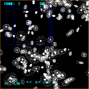
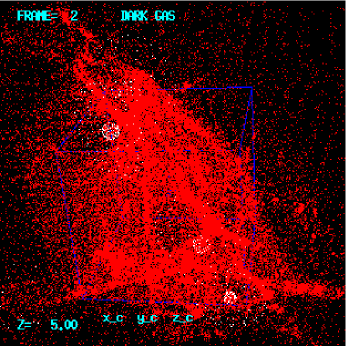
Figure 1: These plots show the reconstruction of a galaxy-galaxy filament present in our 40 Mpc “galaxy” simulation. The cosmology is a standard initially scale-invariant $\Omega_{nr}$=1 CDM model with $\Omega_{B}$=0.05, ${\rm h}$=0.5, normalized to $\sigma_{8}$=0.67. We use the cosmological SPH+P³MultiGrid code described in WB. We identified the peak-patches that should collapse by $z=4$ in the initial conditions (IC), as shown in the top left panel (which is 10 $h^{-1}$Mpc across, comoving). For each patch, the outer ellipsoid represents the alignment of the shear tensor and the inner sphere is an estimate of the final object size. In the lower left panel, we zoom in on the central filamentary web structure and overlay dark matter from a simulation of these IC (panel 2.5 $h^{-1}$Mpc across). The five peak patches (at $z=4$ with overdensity 180) and two voids that define this region were used as constraints for a new higher resolution IC (12.8 Mpc), which we also evolved numerically. These peaks are shown overlaid with dark matter from the new simulation in the right hand panels. The top right panel is a different orientation to the others that shows the filament more clearly, also shown in $n_{HI}$ in Fig. 2. These panels demonstrate that peaks represent an excellent way to compress the essential information about large scale filamentary behaviour.

2 Crafting High Resolution $N$-body/Hydrodynamical Simulations

Although it is usual to evolve ambient “random” patches of the Universe in cosmology, there are obvious advantages in spending one’s computational effort on the regions of most interest. Single peak constraints are very useful if cluster or galaxy formation is the focus, while multiple peak constraints are more useful if superclusters, or cluster substructure, or filaments and walls are the focus. We have seen that the essential features at a given epoch of the filamentary structure and the wall-like webbing between the filaments is largely defined by the dominant collapsed structures, and the peak patches that gave rise to them. A general method for building peak environments is suggested: construct random field initial conditions that require the field to have prescribed values of the peak shear (smoothed over the peak size at the peak position), for a subset from the size-ordered list of peaks that will have a strong impact on the patch to be simulated. Only a handful $N_{pk}$ of peaks and/or voids is usually needed to determine the large scale features, effectively compressing the information needed to $(3+1+6)N_{pk}$ numbers (${\bf r}_{pk},M_{pk},e_{pk,ij}$); peak velocities and the peak constraint are also usually added but these are not as important.

To illustrate how this works, we created a random (unconstrained) initial state for a CDM model in a 40 Mpc box, our “galaxy” simulation. We found peak patches according to the method described in BM and focussed on a specific subregion exhibiting a strong filament, choosing the peaks and voids that were expected to exert strong tidal influences within and upon the patch, as described in Fig. 1. The region chosen was just above the large central cluster of peaks in the top left panel of Fig. 1. We constructed a higher resolution set of “Ly$\alpha$ cloud” initial conditions for this patch, which the “galaxy” initial condition simulation could not resolve well enough to address the low column depth Ly$\alpha$ forest of interest to us.

By compressing the initial data in our target region to just the positions and shears of a few large peak patches, then forming a constrained realization and applying different random waves (optimally-sampled for the smaller region) than the original $40Mpc$ initial condition used, we know we will get high frequency structure wrong. But clearly the large scale features are the same. This is in spite of the tremendously complex filamentary structure just below our chosen sub-region. The peaks we chose were on the basis of rareness (size) and proximity to the patch (using an algorithm roughly based on correlation function falloff from each peak). The five peak-patches used for this companion Ly$\alpha$ simulation had the following masses (in units of $10^{11}{\rm\,M_{\odot}}$) and halo velocity dispersion (in units of $km\,s^{-1}$) as determined from the binding energy: $3.6,77$; $3.5,80$; $1.4,57$; $0.85,48$; $0.51,40$. These accord well with what our group finder finds in the simulation at this redshift. The two void-patches used had Lagrangian masses of $2.4$ and $0.72$, and were outside the high resolution interior. The approximate alignments of the shear tensors for the peak patches inside ensure that a strong filament exists. Fig. 2 shows how the filament looks in HI column density.

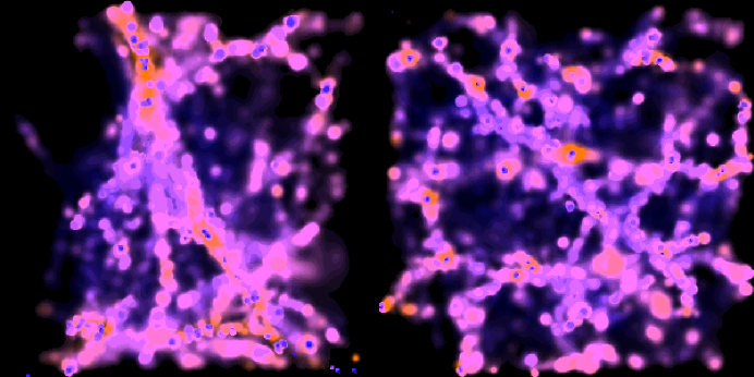
Figure 2: Left: A pseudo ray-traced rendering of the HI density for a region at $z$=4 constrained by the complex pattern of galaxy-scale peak and void shear-fields described in the text, encoding the main large scale structure features, and which ensures strong filamentary webbing arises in the patch. The colour scale codes the temperature variation, with the darker shades in the centre of objects representing high column cold gas. The region is $2.5\,h^{-1}Mpc$ across, comoving, and corresponds to the top right panel of fig. 1. Right: $n_{HI}$ for an ambient patch of the Universe at $z$=3 with control parameter $\nu_{b}$=0, simulation as described in WB. Note the filament dominance in both cases.

To do such complex regions, the standard periodic box approach to cosmological simulations is obviously not appropriate. Advantages of focussed non-periodic simulations include: (1) good mass resolution, allowing us to concentrate on the scale needed to adequately treat the objects that form (e.g. dwarf galaxies, $a_{L}=a_{Lattice,High\,Res}=100$ kpc), and corresponding high numerical resolution ($h_{sph,min}$, $h_{grav}$ $\sim 1$  kpc), can be achieved; (2) good $k$-space sampling is also possible. The competing demands of $k$-space sampling and resolution are further described in Fig. 3. Our method allows high resolution without compromising our long wave coverage by going beyond grid based FFTs, with a FastFT for high $k$ (which kicks out well before the fundamental mode is reached) that is superseded by two direct FTs, power-law then log $k$ sampling, with transitions among them determined by minimizing the volume per mode in $k$-space. Well-sampled $k$-space is especially important for Ly$\alpha$ cloud and galaxy formation as opposed to cluster formation because the density power spectrum for viable hierarchical theories has nearly equal power per decade (approaching flatness in Fig. 3): if just the FFT is used, as is often the case in cosmology even for non-periodic calculations, because there is only one fundamental $k$-mode along each box axis, the large scale structure in the simulation will be poorly modelled, and this can also have a deleterious effect on small scale structure.

There is no point adding long waves without maintaining accurate large scale tides and shearing fields during the calculation. We achieve this with a high resolution region of interest (grid spacing $a_{L}$, $50^{3}$ sphere) that sits within a medium resolution region ($2\,a_{L}$, $40^{3}$), in turn within a low resolution region ($4\,a_{L}$, $32^{3}$). The influence of ultra long waves is included by measuring the mean external tide acting on the low resolution region in the initial conditions, adopting simple models for the ultra-long wave dynamics based on that measurement (e.g. linear, Zeldovich, or homogeneous ellipsoid, as in BM) and applying it as an “external force” throughout the simulation. For this simulation, linear ultra long wave dynamics were adequate.

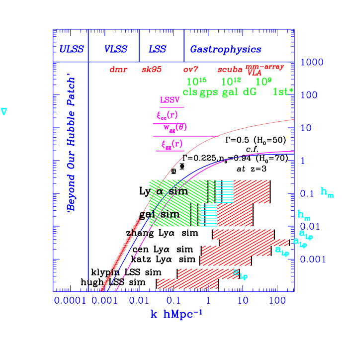
Figure 3: The two (linear) power spectra shown (scaled to redshift 3) were used in the simulations here and in WB. The upper curve at high $k$ is the standard untilted CDM model, but normalized to cluster abundances, $\sigma_{8}=0.67$. The other has the same cosmological age (13 Gyr) and $\Omega_{B}{\rm h}^{2}$ (0.0125) but $H_{0}=70$ with $\Omega_{\Lambda}=0.67$, slightly tilted to be COBE-normalized ($n_{s}=0.94$). (Also shown is a COBE-normalized CDM model, which misses the solid data point in the cluster-band (constraint from $dn_{cl}/dT_{X}$).) The bands in comoving wavenumber probed by various simulations are contrasted. Periodic simulations may use the entire volume, but the $k$-space restriction to lie between the fundamental mode (low-$k$ boundary line) and the Nyquist wavenumber (high-$k$ boundary line) in the IC can severely curtail the rare events in the medium that observations especially probe, and prevents tidal distortions of the simulation volume. We use 3 $k$-space sampling procedures (FFT and two direct FTs) with the boundaries defined by which has the smallest volume per $k$-mode. Even though a $256^{3}$ Fourier transform was used, notice how early the direct sampling takes over (with only 10000 modes). Using an FFT with the very flat spectra in the dwarf galaxy (dG) band can give misleading results. The 3 low-$k$ lines shown for our Ly$\alpha$ and galaxy simulations correspond to the high, medium and low resolution fundamental modes. We actually include modes in the entire hatched region, with the tidal fields associated with the longer waves included by a self-consistent uniform tide on the LR simulation volume. $h_{m}$ denotes our best resolution. $a_{Lp}$ denotes the physical (best) lattice spacing for the grid-based Eulerian hydro codes of Cen and Zhang et.al. ($z=3$). $k$-space domains for two large scale structure ($z=0$) simulations are also shown, a Klypin $256^{3}$ $PM$ calculation and a Couchman (hugh) $128^{3}$ $P^{3}M$ simulation.

In WB, instead of complex multipeak constraints for individual regions, we use importance sampling of shearing patches (patches with the smoothed shear tensor $e_{b,ij}(0)$ prescribed at the centre) to maximize the statistical information we can get from a crafted set of relatively modest constrained-field SPH calculations, defined by a set of control parameters, here the central $\nu_{b}$, $e_{v}$, $p_{v}$ smoothed over a galactic-scale $R_{b}$. This allows us to sample rare peak and void patches, difficult to sample even in large box simulations, especially if FFTs are used. These are in addition to patches with more typical rms density contrasts. We then combine the results to get the frequency distribution of, say, $N_{HI}$ for a random patch of the Universe using Bayes theorem, which decomposes it into the frequency distribution for $N_{HI}$ for our constrained patches given the control parameters, measured from the simulations, and the known probability distribution of the control parameters: schematically,

$P({{\tt random-patch}})=\int P({\tt constr-patch}|{\tt control})\ P({\it\tt control})\ d{\it\tt control-param}$.

Shearing patches with low $|\nu_{b}|$ ${{\raisebox{-3.01385pt}{$<$}}\atop{\raisebox{0.60275pt}{$\sim$}}}2$ often have relatively large shear ellipticity, $\langle e_{v}\,|\nu_{b}\rangle\approx 0.54|\nu_{b}|^{-1}$, which can give strongly asymmetric collapses for $\nu_{b}>0$, amplifying the smaller scale filamentary webbing by concentrating it in larger scale filaments or walls (which depends upon $p_{v}$). Fig. 2 shows that a $\nu_{b}=0$ shearing patch has its $n_{HI}$ filaments more spread out than the multipeak case we have described here, which is reminiscent of, but even more concentrated than, a $\nu_{b}=1.4$ calculation shown in WB.

Simulating a large number of controlled patches in parallel is a form of adaptive refinement, of which there is much discussion in these proceedings. In refined regions, the initial conditions are almost never modified with higher frequency waves, so the Lagrangian (i.e. mass) resolution remains fixed even though the Eulerian resolution may be superb. (This is especially vexing for voids.) When we refine a region by creating a high resolution realization with the information contained in peak patches, we optimally resample $k$-space to generate a new set of high frequency waves. It is clear that the cosmological codes of the future will have to simultaneously adapt in Eulerian and $k$ space, and the techniques explored here offer a promising path towards this goal.