DIRECT Distances to Nearby Galaxies Using Detached Eclipsing Binaries and Cepheids. I. Variables in the Field M31B

Abstract

We undertook a long term project, DIRECT, to obtain the direct distances to two important galaxies in the cosmological distance ladder – M31 and M33, using detached eclipsing binaries (DEBs) and Cepheids. While rare and difficult to detect, detached eclipsing binaries provide us with the potential to determine these distances with an accuracy better than 5%. The massive photometry obtained in order to detect DEBs provides us with good light curves for the Cepheid variables. These are essential to the parallel project to derive direct Baade-Wesselink distances to Cepheids in M31 and M33. For both Cepheids and eclipsing binaries the distance estimates will be free of any intermediate steps.

As a first step of the DIRECT project, between September 1996 and January 1997 we have obtained 36 full nights on the Michigan-Dartmouth-MIT (MDM) 1.3-meter telescope and 45 full/partial nights on the F. L. Whipple Observatory (FLWO) 1.2-meter telescope to search for detached eclipsing binaries and new Cepheids in the M31 and the M33 galaxies. In this paper, first in the series, we present the catalog of variable stars, most of them newly detected, found in the field M31B ($\alpha_{2000.0},\delta_{2000}=11.20\deg,41.59\deg$). We have found 85 variable stars: 12 eclipsing binaries, 38 Cepheids and 35 other periodic, possible long period or non-periodic variables. The catalog of variables, as well as their photometry and finding charts, are available using the anonymous ftp service and the WWW.

1 Introduction

The two nearby galaxies – M31 and M33, are stepping stones to most of our current effort to understand the evolving universe at large scales. First, they are essential to the calibration of the extragalactic distance scale (Jacoby et al. 1992; Tonry et al. 1997). Second, they constrain population synthesis models for early galaxy formation and evolution, and provide the stellar luminosity calibration. There is one simple requirement for all this – accurate distances.

Detached eclipsing binaries (DEBs) have the potential to establish distances to M31 and M33 with an unprecedented accuracy of better than 5% and possibly to better than 1%. These distances are now known to no better than 10-15%, as there are discrepancies of $0.2-0.3\;{\rm mag}$ between RR Lyrae and Cepheids distance indicators (e.g. Huterer, Sasselov & Schechter 1995). Detached eclipsing binaries (for reviews see Andersen 1991, Paczyński 1997) offer a single step distance determination to nearby galaxies and may therefore provide an accurate zero point calibration – a major step towards very accurate determination of the Hubble constant, presently an important but daunting problem for astrophysicists (see the papers from the recent “Debate on the Scale of the Universe”: Tammann 1996, van den Bergh 1996).

The detached eclipsing binaries have yet to be used (Huterer, Sasselov & Schechter 1995; Hilditch 1996) as distance indicators to M31 and M33. According to Hilditch (1996), there are about 60 eclipsing binaries of all kinds known in M31 (Gaposchkin 1962; Baade & Swope 1963; Baade & Swope 1965) and only one in M33 (Hubble 1929)! Only now does the availability of large format CCD detectors and inexpensive CPUs make it possible to organize a massive search for periodic variables, which will produce a handful of good DEB candidates. These can then be spectroscopically followed-up with the powerful new 6.5-10 meter telescopes.

The study of Cepheids in M31 and M33 has a venerable history (Hubble 1926, 1929; Gaposchkin 1962; Baade & Swope 1963; Baade & Swope 1965). In the 80’s Freedman & Madore (1990) and Freedman, Wilson & Madore (1991) studied small samples of the earlier discovered Cepheids, to build PL relations in M31 and M33, respectively. However, both the sparse photometry and the small samples do not provide a good basis for obtaining direct BW distances to Cepheids – the need for new digital photometry has been long overdue. Recently, Magnier et al. (1997) surveyed large portions of M31, which have previously been ignored, and found some 130 new Cepheid variable candidates. Their light curves are however rather sparsely sampled and in $V$ band only.

In this paper, first of the series, we present the catalog of variable stars, most of them newly detected, found in one of the fields in M31. In Sec.2 we discuss the selection of the fields in M31 and the observations. In Sec.3 we describe the data reduction and calibration. In Sec.4 we discuss the automatic selection we used for finding the variable stars. In Sec.5 we discuss the classification of the variables, also using well-defined algorithms whenever possible. In Sec.6 we present the catalog of variable stars. Finally, in Sec.7 we discuss the future follow-up observations and research necessary to fully explore the potential offered by DEBs and Cepheids as direct distance indicators.

2 Fields selection and observations

M31 was primarily observed with the McGraw-Hill 1.3-meter telescope at the MDM Observatory. We used the front-illuminated, Loral $2048^{2}$ CCD Wilbur (Metzger, Tonry & Luppino 1993), which at the $f/7.5$ station of the 1.3-meter has a pixel scale of $0.32\;arcsec/pixel$ and field of view of roughly $11\;arcmin$. We used Kitt Peak Johnson-Cousins $BVI$ filters. Some data for M31 were also obtained with the 1.2-meter telescope at the FLWO, where we used “AndyCam” with thinned, back-side illuminated, AR coated Loral $2048^{2}$ CCD. The pixel scale happens to be essentially the same as at the MDM 1.3-meter telescope. We used standard Johnson-Cousins $BVI$ filters.

Figure 1: Fields observed in M31 during Fall 1996 (squares), based on the photometric survey of M31 by Magnier et al. (1992) and Haiman et al. (1994). Only blue stars, with $B-V<0.4$, are shown. Also shown (circles) are Baade’s Fields I, II, III.

Fields in M31 were selected using the MIT photometric survey of M31 by Magnier et al. (1992) and Haiman et al. (1994). Fig.1 shows stars from this survey with $B-V<0.4$, i.e. blue stars belonging to M31. We selected six $11^{\prime}\times 11^{\prime}$ fields, M31A–F, four of them (A–D) concentrated on the rich spiral arm, one (E) coinciding with the region of M31 searched for microlensing by Crotts & Tomaney (1996), and one (F) containing the giant star formation region known as NGC206 (observed by Baade & Swope 1963). Fields A–C were observed during September and October 1996 5–8 times per night in the $V$ band, resulting in total of 130-160 V exposures per field. Fields D–F were observed once a night in the $V$ band. Some exposures in $B$ and $I$ bands were also taken. M31 was also occasionally observed at the FLWO 1.2-meter telescope, whose main target was M33.

In this paper we present the results for the most frequently observed field, M31B. We obtained for this field useful data during 29 nights at the MDM, collecting a total of 160 $900\;sec$ exposures in $V$, 27 $600\;sec$ exposures in $I$ and 2 $1200\;sec$ exposures in $B$. We also obtained for this field useful data during 14 nights at the FLWO, collecting a total of 4 $900\;sec$ exposures in $V$ and 17 $600\;sec$ exposures in $I$. The complete list of exposures for this field and related data files are available through anonymous ftp on cfa-ftp.harvard.edu, in pub/kstanek/DIRECT directory. Please retrieve the README file for instructions. Additional information on the DIRECT project is available through the WWW at http://cfa-www.harvard.edu/~kstanek/DIRECT/.

3 Data reduction, calibration and astrometry

3.1 Initial reduction, PSF fitting

Preliminary processing of the CCD frames was done with the standard routines in the IRAF-CCDPROC package. For all filters the flatfield frames were prepared by combining “dome flats” and exposures of the twilight sky. These reductions reduced total instrumental systematics to below 1%. The bad columns and hot/cold pixels were masked out using the IRAF routine IMREPLACE.

Stellar profile photometry was extracted using the Daophot/Allstar package (Stetson 1987, 1991). The analyzed images showed a significant positional dependence of the point spread function (PSF), which was well fit by a Moffat-function PSF, quadratically varying with $X,Y$. We selected a “template” frame for each filter using a single frame of particularly good quality. These template images were reduced in a standard way. A set of approximately 100 relatively isolated stars was selected to build the PSF for each image. The PSF star lists as well as lists of objects measured on template images were then used for reduction of remaining, “non-template”, images. For each individual image we first ran FIND and PHOT programs to obtain a preliminary list of stellar positions, then the stars from the “master” PSF list for a given filter were automatically identified, and the PSF was derived. Next for each frame we executed the Allstar program to obtain improved positions for the stars. These positions were used to transform coordinates of the stars included on the “master” list into the coordinates of the current frame. Allstar was then ran in the fixed-position-mode using as an input the transformed “master” list, and the resulting output file contained photometry only for stars measured on the “template” images. There are two classes of objects which may be missed: a) objects located outside ”template” images but inside the present image; and b) objects located inside the “template” field but not included on the master list. By carefully positioning the telescope the offsets between images were small, and in most cases did not exceed 15 pixels. We were, however, concerned about potential variables, such as novae, which could be un-measurable on “template” frames but measurable on some fraction of images. To avoid losing such objects we updated the master list by adding object found by Daophot/Allstar in the “non-fixed-position” mode, detected above $10\sigma$ threshold in the residual images left after subtracting the objects on the current “master” list. Next, Allstar was ran again in the “non-fixed-position” mode using the extended list of stars. Some additional fraction of faint “template” objects was usually rejected by Allstar at this step. As the end result of this procedure we had for each of processed frames (with exception of template images) two lists of photometry: one list including exclusively “template” objects and one including mixture of “template” and “non-template” stars.

Both lists of instrumental photometry derived for a given frame were transformed to the common instrumental system of the appropriate “template” image. As it turned out the offsets of instrumental magnitudes were slightly position dependent and changed by $<0.04\;{\rm mag}$ across a field. This effect was taken into account while transforming photometry to the instrumental system of “template” images. We traced down the source of this problem and found that it is caused by non-perfect modeling of variable PSF in the corners of the images. This means also that photometry derived from “template” images is affected by systematic, position dependent errors. The problem could be cured if it were possible to determine accurate aperture corrections for a large number of stars distributed uniformly over the whole field. Unfortunately this was not the case with our images of M31. The observed fields are very crowded and their images contain limited number of stars with very high S/N. To estimate the size of systematic errors in our photometry we analyzed a set of images of the open cluster NGC 6791 also taken with the MDM 1.3-meter telescope (Kaluzny et al. 1997). The images of NGC 6791 are moderately crowded and contain few hundred stars with S/N sufficiently high for the determination of aperture corrections. Based on examination of the derived aperture corrections and on comparison of profile photometry of NGC 6791 with the photometry of this cluster available in literature (Kaluzny & Rucinski 1995) we concluded that the systematic errors for stars located in corners of M31 fields are $<0.05\;{\rm mag}$.

Photometry obtained for $V$ and $I$ filters was combined into data bases. Two data bases were prepared for each of the filters. One included only photometry for the “template” stars obtained by running Allstar in a “fixed-position-mode”, and second included mixture of “template” and “non-template” objects and was obtained by running Allstar in the “non-fixed-position” mode. In this paper we search for variables only in the first database, i.e. for the “template” stars only.

3.2 Photometric calibration and astrometry

On the night of Sept. 14/15, 1996 we observed 4 Landolt (1992) fields containing a total of 18 standards stars. These fields were observed through the $BV$ filters at air-masses ranging from 1.12 to 1.75, and through the $I$ filter at air masses ranging from 1.12 to 1.53. The following transformation from the instrumental to the standard system was derived:

$$b-v=0.231+0.648(B-V)+0.15X$$ (1)

$$v=V+3.128-0.007(V-I)+0.13X$$ (2)

$$v-i=0.152+1.007(V-I)+0.08X$$ (3)

$$i=I+2.969-0.010(V-I)+0.05X$$ (4)

where lower case letters correspond to the instrumental magnitudes and $X$ is the air mass. It was possible to derive with confidence extinction coefficient for the $V$ filter only. Extinction coefficients for the $B$ and $I$ filters were assumed. In Fig.3 we show the residuals between the standard and calculated magnitudes and colors for the standard stars. The derived transformation satisfactorily reproduces the $V$ and $I$ magnitudes and $V-I$ colors. The $B-V$ transformation reproduces the standard system poorly, due to a rapid decline of quantum efficiency of the Wilbur CCD camera in the range of wavelengths corresponding to the $B$ band. We therefore decided to drop the $B$ data from our analysis of M31B, especially since we took only 2 $B$ frames for this field. We note that all frames of M31 used for calibration of $VI$ photometry were obtained in parallel with observations of Landolt standards and over the air masses not exceeding 1.25. Hence, the fact that we used assumed extinction for the $I$ band is unlikely to introduce any error of the zero point exceeding $0.01\;{\rm mag}$ into M31 photometry. In fact the dominant error of the zero points of the $VI$ photometry for M31 fields are uncertainties of aperture corrections and systematic errors of profile photometry for stars positioned in the corners of the images. We estimate that these external errors of $V$ and $I$ magnitudes are not worse than $0.05\;{\rm mag}$.

Figure 2: Residuals between the standard and calculated magnitudes and colors for 18 standard stars (Landolt 1992) observed on Sept. 14/15, 1996.

Figure 3: $V,V-I$ color-magnitude diagram for $\sim 3,700$ stars in the field M31B. The dashed line corresponds to the $I$ detection limit of $I\sim 21\;{\rm mag}$.

The $V,\;V-I$ color-magnitude diagram based on photometry extracted from the “template” images is shown in Fig.3. The dashed line corresponds to the $I$ detection limit of $I\sim 21\;{\rm mag}$ (see the next section). Stars near $V\sim 22$ and $V-I\sim 1.8$ represent the top of the evolved red giant population. The vertical strip of stars between $0.6<V-I<1.2$ and $V<20$ are the Galactic foreground stars. Stars bluer than $V-I<0.6$ are the upper main sequence, OB type stars, in M31.

We decided to verify our photometric calibration by matching our stars to the photometric survey of Magnier et al. (1992) (hereafter referred to by Ma92) and comparing their photometry. Looking at the upper panel of Fig.4, we can see that the $V$ band photometry matches satisfactorily, and for 92 matched stars with $V<20$ the average difference between “our” $V$ and the $V$ values measured by Ma92 is $0.013\;{\rm mag}$. On the other hand, there is a strong disagreement between the $V-I$ colors for 303 common stars (lower panel of Fig.4). We therefore decided to recheck our calibrations using a different set of calibration frames. During one of the photometric nights (Oct. 2/3, 1996) at the MDM observatory we took a set of calibration frames with the Charlotte $1024\times 1024$ thinned, backside illuminated CCD, which has a pixel scale of $0.5\;arcsec/pixel$. These calibration frames were reduced in the same way as described above for the Wilbur chip and the transformation from the instrumental to the standard system was derived. Comparing to the transformation for the Wilbur CCD, there was an offset of $0.04\;{\rm mag}$ in $V$ and $-0.016\;{\rm mag}$ in $V-I$. This shift of zero points, similar for $V$ and $I$ photometry, is mainly due to the uncertainties in the aperture corrections, which we believe are better derived for the Wilbur CCD, which has smaller pixels. Apart from this offset, we do not see anything resembling the strong trend between the $V-I$ residuals and the $V-I$ color, as seen in the lower panel of Fig.4. This discrepancy certainly deserves further attention.

Figure 4: Residuals between the standard $V$ and $V-I$ obtained for the same stars by us and by Magnier et al. (1992). The agreement for the $V$ values is very good, while there is a strong discrepancy in the values of $V-I$. For discussion see text.

Additional consistency check comes from comparing our photometry from the overlapping regions between the fields (Fig.1). We compared $\sim 170$ common stars in the overlap region between the fields M31B and M31C. There was an offset of $0.034\;{\rm mag}$ in $V$ and $0.024\;{\rm mag}$ in $I$, i.e. within our estimate of $0.05\;{\rm mag}$ discussed above.

Finally, as the last part of the calibration for this field, the equatorial coordinates were calculated for all objects included in the data bases for the $V$ filter. The transformation from rectangular coordinates to equatorial coordinates was derived using 236 stars identified in the list published by Magnier et al. (1992), and the adopted frame solution reproduces equatorial coordinates of these stars with residuals not exceeding $1.0\;arcsec$.

4 Selection of variables

Figure 5: Distributions in $V$ (continuous line) and $I$ (dashed line) of stars in the field M31B.

The reduction procedure described in Section 3 produces databases of calibrated $V$ and $I$ magnitudes and their standard errors. For the moment we are mostly interested in periodic variable stars, so we use only the “first” database, which includes only “template” stars and was obtained by running Allstar in a “fixed-position-mode”. The $V$ database contains 8522 stars with up to 160 measurements, and the $I$ database contains 18815 stars with up to 27 measurements. Fig.5 shows the distributions of stars as a function of mean $\bar{V}$ and $\bar{I}$ magnitude. As can be seen from the shape of the histograms, our completeness starts to drop rapidly at about $\bar{V}\sim 22$ and $\bar{I}\sim 20.5$. The primary reason for this difference in the depth of the photometry between $V$ and $I$ is the level of the combined sky and background light from unresolved M31 stars, which is about three times higher in the $I$ filter than in the $V$ filter.

4.1 Removing the “bad” points

The stars measured on each frame are sorted by magnitude, and for each star we compare its Daophot errors to those of 300 stars with similar magnitude located symmetrically on both sides of a given star in the sorted list. If the Daophot errors for a given star are unusually large, the measurement is flagged as “bad”, and is then removed when analyzing the lightcurve. For each star the remaining measurements are sorted by their error, and the average error and its standard deviation are calculated. Measurements with errors exceeding the average error by more than $4\sigma$ are removed, and the whole procedure is repeated once. Usually 0–10 points are removed, leaving the majority of stars with roughly $N_{good}\sim 150-160$ measurements. For further analysis we use only those stars which have at least $N_{good}>N_{max}/2\;(=80)$ measurements. There are 7208 such stars in the $V$ database of the M31B field.

4.2 Stetson’s variability index

Our next goal is to select objectively a sample of variable stars from the total sample defined above. There are many ways to proceed, and we will largely follow the approach of Stetson (1996), which is in turn based on the Welch & Stetson (1993) algorithm.

We present only a basic summary of Stetson’s (1996) procedure (his Section 2). For each star one can calculate the variability index

$$J=\frac{\sum_{k=1}^{n}w_{k}sgn(P_{k})\sqrt{|{P_{k}}|}}{\sum_{k=1}^{n}w_{k}},$$ (5)

where the user has defined $n$ pairs of observations to be considered, each with a weight $w_{k}$,

$$P_{k}=\left\{\begin{array}[]{ll}\delta_{i(k)}\delta_{j(k)},&\mbox{if $i(k)\neq j(k)$}\\ \delta_{i(k)}^{2}-1,&\mbox{if $i(k)=j(k)$}\end{array}\right.$$ (6)

is the product of the normalized residuals of the two paired observations $i$ and $j$, and

$$\delta=\sqrt{\frac{n}{n-1}}\frac{v-\bar{v}}{\sigma_{v}}$$ (7)

is the magnitude residual of a given observation from the average scaled by the standard error. There are several nuances in the whole procedure, and interested reader should consult Stetson’s paper for details.

Following Stetson (1996) we redefine $J$ so it takes into account how many times a given star was measured. This is simply done by multiplying the variability index by a factor $\sum w/w_{max}$, where $w_{max}$ is the total weight a star would have if measured in all images. This gives us the final variability index

$$J_{S}=J\frac{\sum w}{w_{max}}.$$ (8)

Note that we did not include the measure of the kurtosis of the magnitude for a given star into the definition of $J_{S}$, as proposed by Stetson (1996). We found that including this additional factor made little change to the total number of stars above certain threshold $J_{S,min}$, but tended to remove some of the eclipsing variables from the sample.

To be precise, we should describe how we pair the observations and what weights $w_{k}$ we attach to them. Our observing strategy was designed to have a $V$ image of the M31B field approximately once an hour, so if two $V$ observations are within $1.5\;hour$ from each other, we consider them a pair. However, we pair only the subsequent measurements, so from three closely spaced observations $abc$ we would select two pairs $ab$ and $bc$, but not $ac$. In case when $i(k)\neq j(k)$, we put $w_{k}=1.0$, in case of $i(k)=j(k)$, we put $w_{k}=0.25$. This gives greater weight to longer sequences of closely spaced observations than to the same number of separated observations, for example a sequence $abcd$ would have a total weight of 3.0, while a sequence of $a\;b\;c\;d$ would have the total weight of 1.0.

4.3 Rescaling of Daophot errors

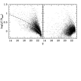
Figure 6: Reduced $\chi^{2}/N_{DOF}$ vs. average magnitude $\bar{V}$ for stars with $N_{good}>80$ measurements. Left panel shows the uncorrected $\chi^{2}/N_{DOF}$, the right panel shows the $\chi^{2}/N_{DOF}$ after the Daophot errors were rescaled. The average correction to the $\chi^{2}/N_{DOF}$ is shown in the left panel with dashed line. For details see text.

The definition of $\delta$ (Eq.7) includes the standard errors of individual observations. If, for some reason, these errors were over- or underestimated, we would either miss real variables, or select spurious variables as real ones. If the standard errors are over- or underestimated by the same factor, we could easily correct the results by changing the cutoff value of the variability index $J_{S}$ (Eq.8). However, this is not the case for our data. In the left panel of Fig.6 we plot the logarithm of the $\chi^{2}/N_{DOF}$ for stars with $N_{good}>80$ measurements. The brightest stars ($V\sim 15$) have $\chi^{2}/N_{DOF}\sim 10$, so their errors are underestimated by roughly $\sqrt{10}$, while stars close to the detection limit, $V\sim 23$, have $\chi^{2}/N_{DOF}<1$ which are too small. Whatever the reasons for this correlation, and there are many possibilities (underestimated flat-fielding errors, less then perfect PSF fits etc.), we will try to account for the problem in purely empirical way, by treating the majority of stars as constant, assuming that for this majority the errors are (roughly) Gaussian. The procedure we apply was described in detail by Lupton et al. (1989), p.206, and it was used before by Udalski et al. (1994). We find that the Daophot error $\sigma_{D}$ might be used as the real observational error provided it is multiplied by an appropriate scaling factor $F$.

Figure 7: Scaling factor $F$ of Daophot errors as a function of average magnitude $\bar{V}$ (see text for details).

In Fig.7 we show the scaling factor $F$ as a function of average magnitude $\bar{V}$. There is a very clear correlation between the $F$ and $\bar{V}$, to which we fitted a linear relation $F=5.88-0.22\bar{V}$. In the right panel of Fig.6 we plot the logarithm of the $\chi^{2}/N_{DOF}$ after the errors were rescaled. Clearly the distribution now is closer to what one would expect from Gaussian population with some variable stars present. However, we do not use rescaled $\chi^{2}/N_{DOF}$ for selecting the variable stars. For that we will use the Stetson’s $J_{S}$ (Eq.8) instead. Using Stetson’s $J_{S}$ allows to effectively remove spurious variability caused by few isolated outstanding points, a property that the $\chi^{2}$ technique does not have.

4.4 Selecting the variables

Figure 8: Variability index $J_{S}$ vs. mean $\bar{V}$ magnitude for stars with $N_{good}>80$, plotted for the real data (upper panel) and the simulated Gaussian noise. In the case of real data, there are stars with $J_{S}>2$ which are not shown. The dashed line at $J_{S}=0.75$ defines the cutoff for variability we use.

We selected the candidate variable stars by computing the value of $J_{S}$ for the stars in our $V$ database. In Fig.8 we plot the variability index $J_{S}$ vs. apparent visual magnitude $\bar{V}$ for stars with $N_{good}>80$, for real data (upper panel) and simulated Gaussian noise (lower panel). In the case of real data, there are stars with $J_{S}>2$ which are not shown. As expected (see discussion in Stetson 1996), most of the stars have values of $J_{S}$ which are close to 0. Not surprisingly, the values of $J_{s}$ for the real data are much more scattered, both due to the real variability, as well as various un-modelled measurement errors.

We used a cutoff of $J_{S,min}=0.75$ to select 202 candidate variable stars (about 3% of the total number of 7208). There is one star with abnormally negative value of $J_{S}$, located at $(\bar{V},J_{S})=(17.86,-1.09)$ in Fig.8, a contact binary with period of $P=0.23\;day=5.5\;hour$ that is comparable to our pairing interval of $1.5\;hour$. We decided to add this star to our sample of candidate variables.

After a preliminary examination of the 203 candidate variables, we decided to add two additional cuts. First, there are in our sample many bright stars with variability of very small ($<0.03\;{\rm mag}$) amplitude. The small variability might be real, since there are other bright stars which show a random scatter of only $\sim 0.01\;{\rm mag}$. We decided, however, to remove variables for which the standard deviation $\sigma$ of the magnitude measurements was smaller than $\sigma<0.03\;{\rm mag}$. Second, we decided to remove from the sample all the stars with the $x$ coordinate greater than $x>2000$. Out of 56 stars with $x>2000$, 25 were classified as variable ($J_{S}>0.75$), and the rest also had larger than normal values of $J_{S}$. The anomalous properties are probably caused by especially strong spatial variation of the PSF near this edge of the CCD. The other edges of the CCD do not show such strong effect. We are left with 163 candidate variable stars.

5 Period determination, classification of variables

5.1 Additional data

We based our candidate variables selection purely on the $V$ band data collected at the MDM telescope. However, to better determine the possible periods and to classify the variables, we added up to 6 $V$ band measurements taken at the FLWO telescope, which extended the time span of observations for some stars to $56\;days$.

We also have the $I$ band data for the field, up to 27 MDM epochs and up to 17 FLWO epochs. As discussed earlier in this paper, the $I$ photometry is not as deep as the $V$ photometry, so some of the candidate variable stars do not have an $I$ counterpart. We will therefore not use the $I$ data for the period determination and broad classification of the variables. We will however use the $I$ data for the “final” classification of some variables.

5.2 Period determination

Next we searched for the periodicities for all 163 candidate variables, using a variant of the Lafler-Kinman (1965) technique proposed by Stetson (1996). Starting with the minimum period of $0.25\;days$, successive trial periods are chosen so

$$P_{j+1}^{-1}=P_{j}^{-1}-\frac{0.01}{\Delta t},$$ (9)

where $\Delta t=t_{N}-t_{1}$ is the time span of the series. The maximum period considered is $\Delta t$. For each trial period, the measurements are sorted by phase and we calculate

$$S(P)=\frac{\sum_{i=1}^{N}w(i,i+1)|m_{i}-m_{i+1}|}{\sum_{i=1}^{N}w(i,i+1)},$$ (10)

where

$$w(i,i+1)=\left[\frac{1}{\sigma_{i}^{2}+\sigma_{i+1}^{2}}\right].$$ (11)

We did not use the additional phase difference weighting proposed by Stetson (1996), because it tends to favor periods longer than the “true” period. For all trial periods the values of $S(P)$ are calculated, and 10 periods corresponding to the deepest local minima of $S(P)$, separated from each other by at least $0.2/\Delta t$, are selected. These 10 periods are then used in our classification scheme.

5.3 Classification of variables

The variables we are most interested in are Cepheids and eclipsing binaries (EBs). We therefore searched our sample of variable stars for these two classes of variables. As mentioned before, for the broad classification of variables we restricted ourselves to the $V$ band data. We will, however, present and use the $I$ band data, when available, when discussing some of the individual variable stars.

5.3.1 Cepheid-like variables

In the search for Cepheids we followed the approach by Stetson (1996) of fitting template light curves to the data. We used the parameterization of Cepheid light curves in the $V$ band as given by Stetson (1996). Any template Cepheid light curve is determined by four parameters: the period, the zero point of the phase, the amplitude and the mean magnitude. From the template Cepheid we calculated the expected magnitude of a Cepheid of the given parameters, and the reduced $\chi^{2}/N_{DOF}$ for the fit of the model light curve to the data. We minimize $\chi^{2}/N_{DOF}$ with a multidimensional minimization routine. We started the minimization with the ten best trial periods from the Lafler-Kinman technique and we also used one half of each value. After finding the best fit we classified the star as a Cepheid if the reduced $\chi^{2}/N_{DOF}$ of the fit was factor of 2 smaller than the reduced $\chi^{2}/N_{DOF}$ of a straight line fit, including a slope. If a candidate satisfied these requirements we restarted the minimization routine ten times with trial periods close to the best fit period. Finally we required that the amplitude of the best fit light curve was larger than $0.1\;{\rm mag}$.

The template light curves we used were defined for period between 7 and $100\;days$, but we allowed for periods between 4 and $100\;days$. The extension to smaller periods produced believable light curves. As can be seen in the lower panel of Fig.9, the fit of the Cepheid template is not perfect: our data in this case is better than what Stetson’s templates were meant to fit (i.e. sparsely sampled Cepheid lightcurves obtained with the HST). However, for purposes of discovery and period derivation these templates are sufficient.

There was a total of 45 variables passing all of the above criteria. Their parameters and light curves are presented in the Sections 6.2, 6.3.

Figure 9: Examples of fitting the model light curves to an eclipsing binary (upper panel) and to a Cepheid (lower panel). For the details see text.

5.3.2 Eclipsing binaries

For eclipsing binaries we used very similar search strategy. We made the simple assumption that the two stars in the binary system are perfect spheres and have uniform surface brightnesses. This is not a good assumption for detailed studies of the parameters of an EB, but acceptable to calculate model light curves for trial fits. Within our assumption the light curve of an EB is determined by nine parameters: the period, the zero point of the phase, the eccentricity, the longitude of periastron, the radii of the two stars relative to the binary separation, the inclination angle, the fraction of light coming from the bigger star and the uneclipsed magnitude. We derive the orbital elements as a function of time by solving Kepler’s equation. A star was classified as an eclipsing variable if the reduced $\chi^{2}/N_{DOF}$ of the EB light curve was smaller than the reduced $\chi^{2}/N_{DOF}$ of a fit to a Cepheid and if it was smaller by a factor of $4(R_{1}+R_{2})\sin^{2}i$ than the reduced $\chi^{2}/N_{DOF}$ of a fit to a line of constant magnitude. The $R_{1,2}$ are the radii of the two stars in the binary relative to the binary separation and $i$ is the inclination angle. The scaling with the radii and the inclination is necessary because some light curves show shallow and/or narrow eclipses. If a candidate star passed these two criteria we ran the minimization routine ten more times with initial period guesses close to the best fit period. We required that the larger radius was less than 0.9 of the binary separation and that the light of each individual star was less than 0.9 of the total light. We further rejected periods between 0.975 and 1.025 and between 1.95 and $2.05\;days$. This last criterion was implemented to prevent us from classifying as eclipsing binaries slowly varying stars, for which the trial periods close to 1 and $2\;days$ produce spurious eclipsing-like curves.

A total of 12 variables passing all of the above criteria and their parameters and light curves are presented in the Section 6.1. In the upper panel of Fig.9 we show an examples of fitting the model light curves to an eclipsing binary.

5.3.3 Miscellaneous variables

After we selected 12 eclipsing binaries and 45 possible Cepheids, we were left with 106 “other” variable stars. Visual inspection of their phased and unphased light curves revealed both reasonably smooth light curves as well as very chaotic or low amplitude variability. Although we have already selected the variables we are particularly interested in, it is of interest to others researchers to present all highly probable variable stars in our data. We therefore decided, for all variable stars other than Cepheids or eclipsing binaries, to raise the threshold of the variability index to $J_{S,min}=1.2$. This leaves 37 variables which we preliminary classify as “miscellaneous”. One of these stars, V7453 D31B, was clearly periodic, so we decided to classify it as “other periodic variable” (see the Section 6.3). We then decided to go back to the CCD frames and try to see by eye if the inferred miscellaneous variability is indeed there, especially in cases when the light curve is very noisy/chaotic. This is obviously a rather subjective procedure, and readers should employ caution when betting their life savings on the reality of some of these candidates. Note that we did not apply this procedure to the eclipsing or Cepheid variables.

We decided to remove 9 dubious variables from the sample, which leaves 27 variables which we classify as miscellaneous. Their parameters and light curves are presented in the Section 6.4.

6 Catalog of variables

In this section we present light curves and some discussion of the 85 variable stars discovered in our survey. Complete $V$ and (when available) $I$ photometry and $128\times 128\;pixel$ ($\sim 40^{\prime\prime}\times 40^{\prime\prime}$) $V$ finding charts for all variables are available through the anonymous ftp on cfa-ftp.harvard.edu, in pub/kstanek/DIRECT directory. Please retrieve the README file for the instructions and the list of files. These data can also be accessed through the WWW at the http://cfa-www.harvard.edu/~kstanek/DIRECT/.

The variable stars are named according to the following convention: letter V for “variable”, the number of the star in the $V$ database, then the letter “D” for our project, DIRECT, followed by the name of the field, in this case (M)31B, e.g. V888 D31B. Tables 1, 2, 3 and 4 list the variable stars sorted broadly by four categories: eclipsing binaries, Cepheids, other periodic variables and “miscellaneous” variables, in our case meaning “variables with no clear periodicity”. Some of the variables which were found independently by survey of Magnier et al. (1997) are denoted in the “Comments” by “Ma97 ID”, where the “ID” is the identification number assigned by Magnier at al. (1997).

Please note that this is a first step in a long-term project and we are planning to collect additional data and information of various kind for this and other fields we observed during 1996. As a result, the current catalog might undergo changes, due to addition, deletion or re-classification of some variables. Please send an e-mail to K. Z. Stanek (kstanek@cfa.harvard.edu) if you want to be informed of any such (major) changes.

6.1 Eclipsing binaries

In Table 1 we present the parameters of the 12 eclipsing binaries in the M31B field. The lightcurves of these variables are shown in Figs.10–11, along with the simple eclipsing binary models discussed in the Section 5.3.2. The model lightcurves were fitted to the $V$ data and then only a zero-point offset was allowed for the $I$ data. The variables are sorted in the Table 1 by the increasing value of the period $P$. For each eclipsing binary we present its name, 2000.0 coordinates (in degrees), value of the variability index $J_{S}$, period $P$, magnitudes $V_{max}$ and $I_{max}$ of the system outside of the eclipse, and the radii of the binary components $R_{1},\;R_{2}$ in the units of the orbital separation. We also give the inclination angle of the binary orbit to the line of sight $i$ and the ellipticity of the orbit $e$. The reader should bear in mind that the values of $V_{max},\;I_{max},\;R_{1},\;R_{2},\;i$ and $e$ are derived with a straightforward model of the eclipsing system (Section 5.3.2), so they should be treated only as reasonable estimates of the “true” value. As can be seen in Figs.10 and 11, these simple binary models (shown with the thin continuous lines) do a reasonable job in most of the cases. More detailed modeling will be performed of the follow-up observations planned (see Section 7).

Figure 10: $V,I$ lightcurves of eclipsing binaries found in the field M31B. The thin continuous line represents for each system the best fit curve (fitted to the $V$ data).

Figure 11: Continued from Fig.10.

6.2 Cepheids

In Table 2 we present the parameters of 38 Cepheids in the M31B field, sorted by the period $P$. For each Cepheid we present its name, 2000.0 coordinates, value of the variability index $J_{S}$, period $P$, flux-weighted mean magnitudes $\langle V\rangle$ and (when available) $\langle I\rangle$, and the amplitude of the variation $A$. In Figs.12–18 we show the phased $V,I$ lightcurves of our Cepheids. Also shown is the best fit template lightcurve (Stetson 1996), which was fitted to the $V$ data and then for the $I$ data only the zero-point offset was allowed.

6.3 Other periodic variables

For some of the variables preliminary classified as Cepheids (Section 5.3.1), we decided upon closer examination to classify them as “other periodic variables”. This category includes also the brightest variable star in the sample, V7453 D31B, which is a RR Lyr star. In Table 3 we present the parameters of 8 possible periodic variables other than Cepheids and eclipsing binaries in the M31B field, sorted by the increasing period $P$. For each variable we present its name, 2000.0 coordinates, value of the variability index $J_{S}$, period $P$, error-weighted mean magnitudes $\bar{V}$ and (when available) $\bar{I}$. To quantify the amplitude of the variability, we also give the standard deviations of the measurements in the $V$ and $I$ bands, $\sigma_{V}$ and $\sigma_{I}$.

6.4 Miscellaneous variables

In Table 4 we present the parameters of miscellaneous variables in the M31B field, sorted by the decreasing value of the mean magnitude $\bar{V}$. For each variable we present its name, 2000.0 coordinates, value of the variability index $J_{S}(>1.2)$, mean magnitudes $\bar{V}$ and $\bar{I}$. To quantify the amplitude of the variability, we also give the standard deviations of the measurements in $V$ and $I$ bands, $\sigma_{V}$ and $\sigma_{I}$. In the “Comments” column we give a rather broad sub-classification of the variability: LP – possible long-period variable ($P>55\;days$); IRR – irregular variable.

Figure 12: $V,I$ lightcurves of Cepheid variables found in the field M31B. The thin continuous line represents for each star the best fit Cepheid template (fitted to the $V$ data).

Figure 13: Continued from Fig.12.

Figure 14: Continued from Fig.12.

Figure 15: Continued from Fig.12.

Figure 16: Continued from Fig.12.

Figure 17: Continued from Fig.12.

Figure 18: Continued from Fig.12.

Table 1: DIRECT Eclipsing Binaries in M31B

Name	$\alpha_{2000.0}$	$\delta_{2000.0}$	$J_{S}$	$P$	$V_{max}$	$I_{max}$	$R_{1}$	$R_{2}$	$i$	$e$	Comments
(D31B)	$[\deg]$	$[\deg]$		$[days]$					[deg]
V438	11.0932	41.6475	$-1.09$	0.2327	17.82	16.86	0.63	0.37	50	0.08	W UMa
V6913	11.2717	41.6462	1.08	0.917	20.63	20.06	0.55	0.44	76	0.01
V6846	11.2724	41.5612	1.61	1.769	20.25	20.13	0.51	0.42	79	0.00
V2763	11.1568	41.4962	1.19	2.302	20.51	20.84	0.57	0.39	74	0.00
V7940	11.3023	41.6240	2.08	2.359	19.28	19.19	0.51	0.34	67	0.01
V6840	11.2703	41.6248	5.01	3.096	19.39	19.34	0.51	0.42	80	0.00
V5442	11.2367	41.5197	0.85	4.213	20.30	19.99	0.39	0.29	71	0.02	DEB
V1266	11.1135	41.6023	1.80	4.516	20.04	19.60	0.48	0.36	75	0.00	DEB?
V888	11.1033	41.6506	0.85	4.757	20.01	19.76	0.37	0.30	66	0.03	DEB
V6105	11.2520	41.5276	0.97	5.232	19.70	19.37	0.33	0.29	68	0.07	DEB
V7628	11.2930	41.6131	2.62	6.109	18.81	18.75	0.53	0.47	73	0.01
V4903	11.2240	41.5196	2.40	6.925	20.12	19.50	0.56	0.44	80	0.00	Ma97 96

Note. — V438 D31B is most probably a foreground W UMa contact binary. V2763 D31B is very blue ($V-I\approx-0.3$), and the $I$ band data, being very close to the detection limit, is very noisy. Variables V5442, V1266, V888 and V6105, with periods from $P\approx 4.2\;days$ to $P\approx 5.2\;days$, are probably detached eclipsing binaries (DEBs).

Table 2: DIRECT Cepheids in M31B

Name	$\alpha_{2000.0}$	$\delta_{2000.0}$	$J_{S}$	$P$	$\langle V\rangle$	$\langle I\rangle$	$A$	Comments
(D31B)	[deg]	[deg]		$[days]$
V1207	11.1130	41.5680	0.96	4.516	21.89	20.47	0.30
V765	11.1022	41.6020	1.23	4.669	21.08	19.94	0.21
V7722	11.2972	41.5568	1.01	5.159	21.91	20.58	0.28
V828	11.1048	41.5640	1.31	5.310	20.99	19.97	0.16
V6872	11.2745	41.5124	1.55	5.863	21.63	20.63	0.35
V6851	11.2703	41.6342	1.56	5.941	21.30	20.22	0.35	Ma97 106
V1547	11.1194	41.6089	2.74	6.314	21.17	20.55	0.39
V4651	11.2146	41.5539	1.72	6.317	21.45	20.40	0.39
V4954	11.2250	41.5292	1.90	6.700	20.88	19.99	0.26	Ma97 97
V2929	11.1581	41.6269	2.84	6.789	20.62	19.81	0.28	Ma97 87
V6314	11.2544	41.6416	1.21	7.008	21.13	19.94	0.27
V7845	11.2983	41.6505	1.06	7.267	21.36	$\cdots$	0.25
V1562	11.1229	41.5087	1.23	7.784	21.21	20.43	0.22
V643	11.1021	41.5130	1.85	7.889	20.40	19.52	0.19
V129	11.0909	41.4971	2.27	8.242	20.76	19.59	0.27
V2977	11.1636	41.5022	1.59	8.518	21.84	20.41	0.39
V2682	11.1498	41.6212	1.37	8.610	21.06	20.24	0.20
V3872	11.1886	41.6339	2.14	8.918	20.95	19.88	0.28	Ma97 93
V762	11.1029	41.5792	2.27	9.465	20.86	19.96	0.27
V7553	11.2886	41.6657	1.11	9.482	20.93	19.77	0.18	Ma97 108
V2293	11.1385	41.6261	2.68	10.567	20.63	19.83	0.24	Ma97 86
V410	11.0918	41.6642	3.37	10.792	20.94	20.19	0.38
V1934	11.1291	41.6133	4.02	12.331	20.97	19.84	0.56
V490	11.0963	41.5883	5.01	12.803	20.27	19.29	0.42
V938	11.1078	41.5457	4.03	12.982	19.87	19.20	0.23	Ma97 80
V2048	11.1315	41.6321	1.76	13.524	20.95	19.83	0.25
V6146	11.2524	41.5531	0.99	13.589	21.41	20.02	0.21	Ma97 102
V6379	11.2585	41.5657	2.06	14.796	20.67	19.40	0.29	Ma97 103
V5148	11.2291	41.5531	2.19	16.065	21.16	19.57	0.39	Ma97 98
V6568	11.2635	41.6005	6.45	19.782	20.62	19.42	0.52	Ma97 104
V7209	11.2814	41.5877	3.46	21.06	20.09	19.15	0.29
V5646	11.2414	41.5093	2.06	23.05	20.93	19.52	0.31
V7872	11.2995	41.6419	1.69	25.54	20.01	19.00	0.10
V7184	11.2797	41.6217	5.39	26.11	19.17	18.46	0.28	Ma97 107
V6875	11.2739	41.5348	2.22	26.46	20.84	19.45	0.47
V7975	11.3061	41.5349	1.12	33.84	20.12	19.09	0.12
V6753	11.2710	41.5228	1.76	37.47	20.45	19.55	0.12
V7713	11.2957	41.6041	1.82	57.52	21.18	19.21	0.26

Table 3: DIRECT Other Periodic Variables in M31B

Name	$\alpha_{2000.0}$	$\delta_{2000.0}$	$J_{S}$	$P$	$\bar{V}$	$\bar{I}$	$\sigma_{V}$	$\sigma_{I}$	Comments
(D31B)	[deg]	[deg]		$[days]$
V7453	11.2909	41.5086	16.99	0.579	16.72	16.28	0.26	0.16	RR Lyr
V6518	11.2610	41.6219	0.97	9.686	21.10	20.61	0.16	0.20
V3825	11.1899	41.5375	1.16	22.02	21.44	20.44	0.28	0.25	W Vir?
V7341	11.2835	41.6406	0.77	29.00	21.48	$\cdots$	0.25	$\cdots$
V4773	11.2197	41.5005	2.06	30.26	21.13	20.28	0.36	0.19	RV Tau
V6164	11.2506	41.6245	2.49	32.72	21.44	20.94	0.53	0.44	RV Tau?
V1290	11.1135	41.6162	0.76	44.7	21.38	20.42	0.18	0.11	RV Tau?
V3469	11.1783	41.5376	1.25	48.0	21.68	20.74	0.43	0.38

Table 4: DIRECT Miscellaneous Variables in M31B

Name	$\alpha_{2000.0}$	$\delta_{2000.0}$	$J_{S}$	$\bar{V}$	$\bar{I}$	$\sigma_{V}$	$\sigma_{I}$	Comments
(D31B)	[deg]	[deg]
V5688	11.2417	41.5304	2.34	17.55	16.81	0.05	0.03	Foreground
V4697	11.2172	41.5069	2.31	18.13	17.55	0.05	0.11	Foreground
V6496	11.2638	41.5072	1.71	18.20	15.96	0.04	0.03	LP
V7984	11.3061	41.5425	4.66	18.20	17.09	0.10	0.08	IRR
V7606	11.2911	41.6454	1.28	19.03	16.81	0.06	0.03	LP
V5830	11.2449	41.5139	2.02	19.07	16.75	0.08	0.04	LP
V8123	11.3081	41.6494	2.42	19.12	17.27	0.10	0.07	LP
V1019	11.1073	41.6165	2.08	19.17	17.41	0.09	0.06	LP
V8197	11.3121	41.6263	1.45	19.45	16.35	0.08	0.04	LP
V4062	11.1987	41.5138	3.60	19.75	16.72	0.13	0.05	LP
V7326	11.2839	41.6152	1.29	19.77	17.13	0.07	0.03	LP
V6936	11.2726	41.6354	1.32	19.80	19.38	0.08	0.09	IRR
V7797	11.2979	41.6375	1.23	20.04	20.57	0.09	0.13	blue
V5724	11.2396	41.6256	1.41	20.31	19.41	0.20	0.09	LP
V3333	11.1717	41.6167	4.06	20.82	20.23	0.64	0.41	LP
V5504	11.2382	41.5095	1.30	20.95	18.52	0.19	0.17	LP
V3237	11.1698	41.5627	2.03	20.99	20.23	0.24	0.35	Ma97 89
V6222	11.2511	41.6549	1.38	21.04	20.02	0.27	0.16	LP
V4309	11.2062	41.5118	1.39	21.29	19.80	0.63	0.17	LP
V4719	11.2169	41.5402	1.52	21.39	20.30	0.45	0.13	LP
V4669	11.2920	41.5467	1.22	21.40	19.48	0.27	0.16	LP
V5897	11.2424	41.6594	1.98	21.56	19.22	0.54	0.16	LP
V7745	11.2991	41.5104	2.01	21.72	19.60	0.41	0.11	LP
V2356	11.1412	41.5966	1.22	21.73	19.53	0.54	0.17	LP
V7746	11.2982	41.5416	1.31	21.83	19.92	0.38	0.17	LP
V5075	11.2239	41.6504	1.31	21.85	19.31	0.48	0.09	LP
V4690	11.2142	41.5988	1.88	21.90	19.78	0.48	0.14	LP

Figure 19: $V,I$ lightcurves of other periodic variables found in the field M31B.

Figure 20: Continued from Fig.19.

Figure 21: $V,I$ lightcurves of miscellaneous variables found in the field M31B.

Figure 22: Continued from Fig.21.

Figure 23: Continued from Fig.21.

Figure 24: Continued from Fig.21.

Figure 25: Continued from Fig.21.

6.5 Comparison with other catalogs

The M31B field has not been observed frequently before and the only overlapping variable star catalog is given by Magnier et al. (1997, hereafter Ma97). Of 16 variable stars in Ma97 which are in our M31B field, we cross-identified 15. Of these 15 stars, one (Ma97 101) we did not classify as a variable ($J_{S}=0.49$), one (V4903 D31B = Ma97 96) was classified as an eclipsing binary and one (V3237 D31B = Ma97 89) we classified as miscellaneous variable. The remaining 12 stars we classified as Cepheids (see Table 2 for cross-identifications). Our M31B field also includes a confirmed Luminous Blue Variable (see Humpreys & Davidson 1994 for a review), M31 Var A-1 (Humpreys 1997, private communication). We cross-identified M31 Var A-1 in our data and found it to be non-variable, with average magnitudes $\bar{V}=16.80,\;\bar{I}=16.10$.

7 Discussion, follow-up observations and research

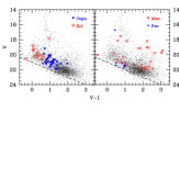
Figure 26: $V,\;V-I$ color-magnitude diagrams for the variable stars found in the field M31B. The eclipsing binaries and Cepheids are plotted in the left panel and the other periodic variables and miscellaneous variables are plotted in the right panel. The dashed line corresponds to the $I$ detection limit of $I\sim 21\;{\rm mag}$.

In Fig.26 we show $V,\;V-I$ color-magnitude diagrams for the variable stars found in the field M31B. The eclipsing binaries and Cepheids are plotted in the left panel and the other periodic variables and miscellaneous variables are plotted in the right panel. As expected, the eclipsing binaries, with the exception of the foreground W UMa system V438 D31B, occupy the blue upper main sequence of M31 stars. Also as expected, the Cepheid variables group near $V-I\sim 1.0$, with the exception of possibly highly reddened system V7713 D31B. The other periodic variable stars have positions on the CMD similar to the Cepheids, again with the exception of the foreground RR Lyr V7553 D31B. The miscellaneous variables are scattered throughout the CMD and clearly represent many classes of variability, but most of them are red with $V-I=1.6-3.2$, and are probably Mira variables.

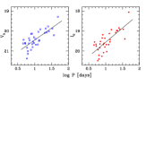
Figure 27: The PL relations in the $V$ and $I$ bands for 34 Cepheids in field M31B. A preliminary estimate of the extinction has been used (see text for more details).

The classical Cepheids found span pulsation periods from 4.5 to $57\;days$ and all of them appear to be fundamental mode pulsators. The period-luminosity [PL] relations (in the $V$ and $I$ bands) for the 34 Cepheids in field M31B are shown in Fig.27. They resemble the PL relations in Field III of Freedman & Madore (1990), which contain 16 Cepheids observed in $BVRI$ filters. The distribution of the V and I residuals is also similar to that found by Gould (1994) for Field III. Using the technique described in Sasselov et al. (1996), and adopting M31 foreground extinction $E(B-V)=0.08$ and no depth dispersion, we estimate the mean extinction of the M31B Cepheid sample to be $E(B-V)=0.2$. The range of individual extinctions is very large, up to $E(B-V)=0.6$. By enforcing positivity of the extinction, two of the 36 Cepheids are found to have luminous companions (or blends). The nominal distance difference between LMC and M31 from our sample is $\Delta\mu(M31-LMC)=6.05\pm 0.15$. Due to the still small sample and only two-band photometry these estimates are only preliminary; the final sample from all fields should allow us to derive PL relations to study dependencies as a function of galactocentric position and derive the distance to M31.

At this stage of the DIRECT project we are interested mostly in identifying interesting variable stars in M31 and M33. As we demonstrated 1-meter class telescopes are sufficient for this purpose, providing one can obtain enough telescope time. During the next stage of our project, the most promising detached eclipsing binaries and Cepheid variables will be selected from our M31 and M33 variable star catalogs to do accurate ($\sim 1\%$) follow-up photometry in the $BVI$ bands. A 2-meter class telescope with good seeing will be necessary to obtain enough photometric precision. These accurate light curves will then be used to determine the solutions of photometric orbits of eclipsing binaries, a well-understood problem in astronomy (Wilson & Devinney 1971), as well for the modified Baade-Wesselink technique modelling of the Cepheids (Krockenberger, Sasselov & Noyes 1997).

Another step of this project, which requires obtaining high S/N radial velocity curves to get the radii in physical units, would be realized using one of the new 6.5-10 meter class telescopes. For an idealized DEB system of two identical mass stars viewed exactly in the orbital plane, the expected semi-amplitude of the radial velocity curve is given by

$$K=135\;\left(\frac{M_{star}}{M_{\odot}}\right)^{1/3}\left(\frac{P_{orbital}}{1\;day}\right)^{-1/3}\;km\;s^{-1},$$ (12)

which for late O–early B type binaries typically translates to $\sim 200\;km\;s^{-1}$ (e.g. V478 Cyg or CW Cep, see Andersen 1991). Determining the distance to an accuracy of 5% requires knowing the semi-amplitudes of the radial velocity curve to $\sim 10\;km\;s^{-1}$ – a very demanding, but not impossible task.

The last step would be the calculation of the distances: knowing the surface brightness and the stellar radii of the DEB system or Cepheid we can obtain the absolute stellar luminosities in the observed band $F_{stellar~{}surface}$, and from the apparent fluxes measured $F_{telescope}$ we can directly obtain the distance

$$d=\left({F_{stellar~{}surface}\over F_{telescope}}\right)^{1/2}R_{star}.$$ (13)

This means that we need very accurate absolute photometry from the observed system in some selected band or, better, in several bands. This also means that we have to be able to estimate the surface brightness in some selected band of each star from the observed colors or spectra. Interstellar extinction is always a problem for any photometric distance determination. To correct for that, multi-band absolute photometry outside the eclipses in standard $UBVI$ and possibly $JHK$ will be obtained. De-reddening for early type stars is a standard and simple problem. As M33 is nearly a face-on system, the problems with the interstellar extinction for this galaxy may be less severe than for M31, a galaxy with obvious and patchy extinction.

References

- (1)
- (2) Andersen, J., 1991, A&AR, 3, 91
- (3) Baade, W., Swope, H. H., 1963, AJ, 68, 435
- (4) Baade, W., Swope, H. H., 1965, AJ, 70, 212
- (5) Freedman, W. L., Wilson, C. D., & Madore, B. F., 1991, ApJ, 372, 455
- (6) Freedman, W. L., & Madore, B. F., 1990, ApJ, 365, 186
- (7) Gaposchkin, S., 1962, AJ, 67, 334
- (8) Gould, A. 1994, ApJ, 426, 542.
- (9) Haiman, Z., Magnier, E., Lewin, W. H. G., Lester, R. R., van Paradijs, J., Hasinger, G., Pietsch, W., Supper, R., & Truemper, J., 1994, A&A, 286, 725
- (10) Hilditch, R. W., 1996, in: “Binaries in Clusters”, eds. E. F. Milone & J.-C. Mermilliod (ASP Conference Series Vol. 90), 207
- (11) Hubble, E., 1926, ApJ, 63, 236
- (12) Hubble, E., 1929, ApJ, 69, 103
- (13) Hubble, E., & Sandage, A., 1953, ApJ, 118, 353
- (14) Humpreys, R. M., & Davidson, K., 1994, PASP, 106, 704
- (15) Huterer, D., Sasselov, D. D., Schechter, P. L., 1995, AJ, 100, 2705
- (16) Kaluzny, J., & Rucinski, S. M., 1995, A&AS, 114, 1
- (17) Kaluzny, J., Stanek, K. Z., Garnavich, P., & Challis, P., 1997, ApJ, 491 (to appear in Dec. 10 issue)
- (18) Krockenberger, M., Sasselov, D., & Noyes, R., 1997, ApJ, 479, 875
- (19) Landolt, A., 1992, AJ, 104, 340
- (20) Lupton, R. H., Fall, S. M., Freeman, K. C., & Elson, R. A. W., 1989, ApJ, 370, 201
- (21) Magnier, E. A., Lewin, W. H. G., Van Paradijs, J., Hasinger, G., Jain, A., Pietsch, W., & Truemper, J., 1992, A&AS, 96, 37
- (22) Magnier, E. A., Lewin, W. H. G., van Paradijs, J., Hasinger, G., Pietsch, W., & Trumper, J., 1993, A&A, 272, 695
- (23) Magnier, E. A., Augusteijn, T., Prins, S., van Paradijs, J., & Lewin, W. H. G., 1997, A&A, in press
- (24) Metzger, M. R., Tonry, J. L., & Luppino, G. A., 1993, ASP Conf. Ser., 52, 300
- (25) Paczyński, B., 1997, “The Extragalactic Distance Scale STScI Symposium”, eds. M. Livio, M. Donahue & N. Panagia, in press (astro-ph/9608094)
- (26) Sasselov, D., Beaulieu, J.P., Renault, C., et al. (EROS Team), 1997, A&A, 324, 471
- (27) Stetson, P.B. 1987, PASP, 99, 191
- (28) Stetson, P.B 1991, in “Astrophysical Data Analysis Software and Systems I”, ASP Conf. Ser. Vol. 25, eds. D.M. Worrall, C. Bimesderfer, & J. Barnes, 297
- (29) Stetson, P. B., 1996, PASP, 108, 851
- (30) Tammann, G. A., 1996, PASP, 108, 1083
- (31) Tonry, J. L., Blakeslee, J. P., Ajhar, E. A., & Dressler, A., 1997, ApJ, 475, 399
- (32) Udalski, A., Szymański, M., Stanek, K. Z., Kałużny, J., Kubiak, M., Mateo, M., Krzemiński, W., Paczyński, B., & Venkat, R., 1994, Acta Astron., 44, 165
- (33) van den Bergh, 1996, PASP, 108, 1091
- (34) Wilson, R. E., Devinney, E. J., 1971, ApJ, 166, 605
- (35)