Constraints on the Redshift and Luminosity Distributions of Gamma Ray Bursts in an Einstein-de Sitter Universe

Abstract

Two models of the gamma ray burst population, one with a standard candle luminosity and one with a power law luminosity distribution, are $\chi^{2}$-fitted to the union of two data sets: the differential number versus peak flux distribution of BATSE’s long duration bursts, and the time dilation and energy shifting versus peak flux information of pulse duration time dilation factors, interpulse duration time dilation factors, and peak energy shifting factors. The differential peak flux distribution is corrected for threshold effects at low peak fluxes and at short burst durations, and the pulse duration time dilation factors are also corrected for energy stretching and similar effects. Within an Einstein-de Sitter cosmology, we place strong bounds on the evolution of the bursts, and these bounds are incompatible with a homogeneous population, assuming a power law spectrum and no luminosity evolution. Additionally, under the implied conditions of moderate evolution, the 90% width of the observed luminosity distribution is shown to be $\mathrel{\hbox{\hbox to0.0pt{\hbox{\lower 4.0pt\hbox{$\sim$}}\hss}\hbox{$<$}}}$ 10², which is less constrained than others have demonstrated it to be assuming no evolution. Finally, redshift considerations indicate that if the redshifts of BATSE’s faintest bursts are to be compatible with that which is currently known for galaxies, a standard candle luminosity is unacceptable, and in the case of the power law luminosity distribution, a mean luminosity $\mathrel{\hbox{\hbox to0.0pt{\hbox{\lower 4.0pt\hbox{$\sim$}}\hss}\hbox{$<$}}}$ 10⁵⁷ ph s^-1 is favored.

1 Introduction

The angular distribution of the gamma ray burst population has been shown to be highly isotropic (Meegan et al. (1992); Briggs et al. (1996)). This suggests that the bursts are either located in an extended galactic halo (e.g., Paczyński (1991)) or that they are cosmological in origin (e.g., Paczyński (1986)). Recent measurements of time dilation of burst durations (Norris et al. (1994), 1995; Wijers & Paczyński (1994); however, see Mitrofanov et al. (1996)), of pulse durations (Norris et al. 1996a ), and of interpulse durations (Davis (1995); Norris et al. 1996b ) in the BATSE data, as well as measurements of peak energy shifting (Mallozzi et al. (1995)), favor the latter explanation.

Models, both galactic and cosmological, are typically fitted to the differential peak flux distribution of BATSE’s long duration ($T_{90}>$ 2 s) bursts. Furthermore, this distribution is typically truncated at a peak flux of 1 ph cm^-2 s^-1 to avoid threshold effects. Here, we fit two models, one with a standard candle luminosity and one with a power law luminosity distribution, to not only BATSE’s 3B differential distribution, but also to the pulse duration time dilation factors (corrected for energy stretching and similar effects) of Norris et al. (1996a), the interpulse duration time dilation factors of Norris et al. (1996b), and the peak energy shifting factors of Mallozzi et al. (1995). These three independent sets of measurements are shown to be self-consistent in §4. (All three are for long duration bursts only.) Furthermore, via the analysis of Petrosian & Lee (1996a), BATSE’s differential distribution is extended down to a peak flux of 0.316 ph cm^-2 s^-1, which corresponds to a trigger efficiency of $\sim\frac{1}{2}$ on BATSE’s 1024 ms timescale.

Together, the differential distribution and the time dilation and energy shifting factors place strong bounds on the evolution of the burst population. These bounds favor moderate evolution and are incompatible with homogeneity, assuming only minimal luminosity evolution. This result is compatible with the analyses of Fenimore & Bloom (1995), Nemiroff et al. (1996), and Horack, Mallozzi, & Koshut (1996). Furthermore, under these conditions of moderate evolution, the 90% width of the observed luminosity distribution is shown to be less constrained than others have demonstrated it to be assuming no evolution (see §5). Finally, redshift considerations indicate that if the redshifts of BATSE’s faintest bursts are to be compatible with that which is currently associated with the formation of the earliest galaxies, the mean luminosity of the bursts should be $\sim$ 10⁵⁷ ph s^-1 or lower.

2 Cosmological Models

Both the standard candle luminosity model and the power law luminosity distribution model assume a power law redshift distribution, given by

$$n(z)=n_{0}(1+z)^{D},$$ (1)

where $n(z)$ is the number density of bursts of redshift $z$. This distribution is bounded by 0 $<z<z_{M}$, where $z_{M}$ is the maximum burst redshift. The luminosity distributions of the two models are given by

$$\phi(L)=\cases{\phi_{0}\delta(L-L_{0})&(standard candle)\cr\phi_{0}L^{-\beta}&(power law)}.$$ (2)

The standard candle is of luminosity $L_{0}$ and the power law luminosity is bounded by minimum and maximum luminosities $L_{m}<L<L_{M}$. All luminosities are peak photon number luminosities and all fluxes are peak photon number fluxes (measured over BATSE’s 50 - 300 keV triggering range); however, see recent papers by Bloom, Fenimore, & in ’t Zand (1996) and Petrosian & Lee (1996b) which introduce the fluence measure.

2.1 Integral Distribution

Assuming a power law spectrum and an Einstein-de Sitter cosmology, the bursts’ integral distribution, i.e. the number of bursts with peak fluxes greater than an arbitrary value $F$, is given for either model by (Mészáros & Mészáros (1995))

$$N(>F)=\frac{32\pi n_{0}c^{3}}{H_{0}^{3}}\int_{L_{m}}^{L_{M}}\phi(L)dL\int_{0}^{\chi_{0}}(1-\chi)^{8-2D}\chi^{2}d\chi,$$ (3)

where

$$\chi_{0}=min(\chi_{1},\chi_{2}),$$ (4)

$$\chi_{1}=\frac{1}{1+{\frac{4c}{H_{0}}}\left({\frac{\pi F}{L}}\right)^{\frac{1}{2}}},$$ (5)

and

$$\chi_{2}=1-\frac{1}{(1+z_{M})^{\frac{1}{2}}}.$$ (6)

A photon number spectral index of -1 (or a power-per-decade spectral index of 1) has been assumed. This value is typical of burst spectra, especially at those frequencies at which most of the photons are received (e.g., Band et al. (1993)). In the case of the standard candle model, eq. 3 becomes

$$N(>F)\propto\int_{0}^{\chi_{0}}(1-\chi)^{8-2D}\chi^{2}d\chi,$$ (7)

where $L=L_{0}$ in eq. 5. The factor of proportionality has been dropped because only normalized integral distributions (see §3.1) and ratios of integral distributions (see §2.2) are fit to. Eq. 7 has the analytic solution

$$N(>F)\propto f(\chi_{0},8-2D),$$ (8)

where

$$f(\chi,q)=\frac{2(1-(1-\chi)^{3+q})}{(1+q)(2+q)(3+q)}-\frac{2\chi(1-\chi)^{2+q}}{(1+q)(2+q)}-\frac{\chi^{2}(1-\chi)^{1+q}}{1+q}.$$ (9)

In the case of the power law model, eq. 3 becomes

$$N(>F)\propto\int_{1}^{K}x^{-\beta}dx\int_{0}^{\chi_{0}}(1-\chi)^{8-2D}\chi^{2}d\chi,$$ (10)

where

$$K=\frac{L_{M}}{L_{m}}$$ (11)

and $L=xL_{m}$ in eq. 5. Eq. 10 has the integral solution

$$N(>F)\propto\int_{1}^{K}f(\chi_{0},8-2D)x^{-\beta}dx.$$ (12)

2.2 Time Dilation and Energy Shifting Factors

In an idealized scenario of two identical bursts at different redshifts, $z_{1}$ and $z_{2}$, their time dilation and energy shifting factors, $\tau_{12}$ and $\epsilon_{12}$, are both simply equal to the ratios of their scale factors (neglecting the effects of energy stretching which are inherent in pulse duration measurements (Fenimore & Bloom (1995))):

$$\tau_{12}=\epsilon_{12}^{-1}=\frac{1+z_{1}}{1+z_{2}}.$$ (13)

In practice, however, measures of the scale factor are averaged over peak flux ranges and time dilation and energy shifting factors are determined for pairs of these ranges. Mészáros & Mészáros (1996) demonstrated that such mean values of the scale factor, averaged over a peak flux range $F_{l}<F<F_{u}$, are simple functions of the integral distribution, as modeled by eqs. 8 and 12:

$$\overline{(1+z)}(F_{l},F_{u})=\frac{N_{D+1}(F_{l},F_{u})}{N_{D}(F_{l},F_{u})},$$ (14)

where

$$N(F_{l},F_{u})=N(>F_{u})-N(>F_{l}).$$ (15)

Consequently, time dilation and energy shifting factors between two such ranges, $F_{1,l}<F_{1}<F_{1,u}$ and $F_{2,l}<F_{2}<F_{2,u}$, are given by

$$\tau_{12}=\epsilon_{12}^{-1}=\frac{N_{D+1}(F_{1,l},F_{1,u})N_{D}(F_{2,l},F_{2,u})}{N_{D}(F_{1,l},F_{1,u})N_{D+1}(F_{2,l},F_{2,u})}.$$ (16)

The effects of energy stretching are not modeled here because they are removed empirically from the pulse duration measurements of Norris et al. (1996a) in §3.2. The interpulse duration measurements of Norris et al. (1996b) and the peak energy measurements of Mallozzi et al. (1995) do not require such corrections.

3 Data Analysis

3.1 Integral Distribution

BATSE’s sensitivity becomes less than unity at peak fluxes below $\sim$ 1 ph cm^-2 s^-1 (Fenimore et al. (1993)). Petrosian, Lee, & Azzam (1994) demonstrated that BATSE is additionally biased against short duration bursts: BATSE triggers when the mean photon count rate, defined by

$$\bar{C}(t)=\frac{1}{\Delta t}\int_{t}^{t+\Delta t}C(t)dt$$ (17)

where $\Delta t=$ 64, 256, and 1024 ms are BATSE’s predefined timescales, exceeds the threshold count rate, $\bar{C}_{lim}$, on a particular timescale. Consequently, peak photon count rates are underestimated for bursts of duration $T\mathrel{\hbox{\hbox to0.0pt{\hbox{\lower 4.0pt\hbox{$\sim$}}\hss}\hbox{$<$}}}\Delta t$, sometimes to the point of non-detection. Peak fluxes are similarly underestimated. Petrosian & Lee (1996a) developed (1) a correction for BATSE’s measured peak fluxes and (2) a non-parametric method of correcting BATSE’s integral distribution.

A burst’s corrected peak flux is given by

$$F=\bar{F}\left(1+\frac{\Delta t}{T_{90}}\right),$$ (18)

where $\bar{F}$ is the burst’s measured peak flux and $T_{90}$ is the burst’s 90$\%$ duration. Consequently, if $T_{90}\gg\Delta t$, $F\simeq\bar{F}$; however if $T_{90}\mathrel{\hbox{\hbox to0.0pt{\hbox{\lower 4.0pt\hbox{$\sim$}}\hss}\hbox{$<$}}}\Delta t$, $F>\bar{F}$. Petrosian & Lee (1996a) demonstrated that eq. 18 adequately corrects BATSE’s measured peak fluxes (1) on the 1024 ms timescale, (2) for bursts of duration $T_{90}>$ 64 ms, and (3) for a variety of burst time profiles.

BATSE’s corrected integral distribution is given by

$$N(>F_{i})=\cases{1&$(i=1)$\cr\prod_{j=2}^{i}(1+\frac{1}{M_{j}})&$(i>1)$},$$ (19)

where $F_{i}>F_{i+1}$, $F_{i}>F_{lim,i}(T_{90})$, and $M_{i}$ is the number of points in the associated set $\cal M$${}_{i}=\{(F_{j},F_{lim,j}(T_{90})):F_{j}>F_{i}$ and $F_{lim,j}(T_{90})<F_{i}\}$. The corrected threshold flux, $F_{lim}(T_{90})$, is the minimum value of the corrected peak flux that satisfies the trigger criterion: $\bar{F}>\bar{F}_{lim}$, where

$$\bar{F}_{lim}=\bar{C}_{lim}\left(\frac{\bar{F}}{\bar{C}}\right)$$ (20)

and $\bar{C}$ is the measured peak photon count rate. By eq. 18, $F_{lim}(T_{90})$ is indeed a function of $T_{90}$ and is similarly given by

$$F_{lim}(T_{90})=\bar{F}_{lim}(1+\frac{\Delta t}{T_{90}}).$$ (21)

We apply the peak flux and integral distribution corrections of Petrosian & Lee (1996a) with one restriction: Kouvelioutou et al. (1993), Petrosian, Lee, & Azzam (1994), and Petrosian & Lee (1996a) have demonstrated that the distribution of BATSE burst durations is bimodal, with the division occuring at $T_{90}\sim$ 2 s. This suggests that short ($T_{90}<$ 2 s) and long ($T_{90}>$ 2 s) duration bursts may be drawn from separate populations. This notion is further supported by the tendency of short duration bursts (1) to have steeper integral distributions than long duration bursts (Petrosian & Lee 1996a ), and (2) to have lower energy shifting factors than long duration bursts, especially at low peak fluxes (Mallozzi et al. (1995)). Consequently, we exclude short duration bursts from our sample.

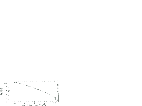
Figure 1: Uncorrected and corrected integral distributions of long duration ($T_{90}>$ 2 s) BATSE bursts.

Of the 1122 bursts in the 3B catalog, information sufficient to perform these corrections, subject to the above restriction, exists for 423 bursts. The corrected integral distribution is plotted in fig. 1. It can be seen that the corrected distribution differs significantly from the uncorrected distribution only at peak fluxes below $F\sim$ 0.4 ph cm^-2 s^-1. For purposes of fitting, we truncate and normalize the integral distribution at $F=$ 0.316 ph cm^-2 s^-1, which corresponds to a trigger efficiency of $\sim\frac{1}{2}$. The remaining 397 bursts are divided into eighteen bins: fifteen are of logarithmic length 0.1, and the brightest three are of logarithmic length 0.2.

3.2 Time Dilation and Energy Shifting Factors

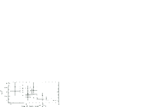
Figure 2: Calibrated (§3.2) pulse duration time dilation factors of Norris et al. (1996a) computed using peak alignment (closed circles) and auto-correlation (open circles) statistics; interpulse duration time dilation factors of Norris et al. (1996b) computed using temporal resolutions of 512 ms (closed squares) and 128 ms (open squares) and signal-to-noise thresholds of 1400 counts s^-1 (closed squares) and 2400 counts s^-1 (open squares); and inverse peak energy shifting factors of Mallozzi et al. (1995) (closed triangles). The time dilation factors and the energy shifting factors have been computed using two different reference bins.

The pulse duration time dilation factors of Norris et al. (1996a), computed using both peak alignment and auto-correlation statistics, are subject to energy stretching: pulse durations tend to be shorter at higher energies (Fenimore et al. (1995)); consequently, pulse duration measurements of redshifted bursts are necessarily underestimated. Furthermore, Norris et al. (1996a) demonstrated that the unavoidable inclusion of the interpulse intervals in these analyses has a similar effect. To correct for these effects, Norris et al. (1996a) provided a means of calibration: they stretched and shifted, respectively, the time profiles and the energy spectra of the bursts of their reference bin by factors of 2 and 3, and from these “redshifted” bursts, they computed “observed” time dilation factors. For each statistic, we have fitted these “observed” time dilation factors to the “actual” time dilation factors of 2 and 3 with a power law which necessarily passes through the origin. Calibrated time dilation factors are determined from these fits and are plotted in fig. 2.

These calibrated time dilation factors are consistent with both the interpulse duration time dilation factors of Norris et al. (1996b) and the energy shifting factors (long duration bursts only) of Mallozzi et al. (1995) (see §4), neither of which require significant energy stretching corrections. The interpulse duration time dilation factors were computed for various combinations of temporal resolutions and signal-to-noise thresholds. Norris et al. (1996b) provided error estimates for two such combinations, which they described as “conservative” with respect to their statistical significance. These time dilation factors and the energy shifting factors of Mallozzi et al. (1995) are additionally plotted in fig. 2. All 22 of the time dilation and energy stretching factors are fit to in §4.

4 Model Fits

Both the standard candle luminosity model and the power law luminosity distribution model have been $\chi^{2}$-fitted to the corrected and binned differential distribution of fig. 1 (see §3.1) and to the time dilation and energy shifting factors of fig. 2 (see §3.2). Additionally, both models have been $\chi^{2}$-fitted to the union of these data sets. In the case of the standard candle model, $\Delta\chi^{2}$ confidence regions, as prescribed by Press et al. (1989), are computed on a 100²-point grid. In the case of the power law model, $\Delta\chi^{2}$ confidence regions are computed on a 50⁴-point grid and are projected into three two-dimensional planes.

4.1 Standard Candle Luminosity Model

The standard candle model consists of three parameters: $h^{2}L_{0}$, $D$, and $z_{M}$, where $h=H_{0}/100$. By eqs. 5 and 6, $z_{M}$ is constrained by

$$z_{M}>\left(1+\frac{H_{0}}{4c}\left(\frac{L_{0}}{\pi F_{m}}\right)^{\frac{1}{2}}\right)^{2}-1,$$ (22)

where $F_{m}=$ 0.201 ph cm^-2 s^-1 is the peak flux of BATSE’s faintest burst. However, above this limit, $z_{M}$ is independent of the data.

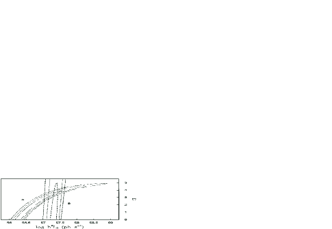
Figure 3: $\Delta\chi^{2}$ confidence regions of the standard candle model fit to the differential distribution (A) and to the time dilation and energy shifting factors (B). Dotted lines are 1-$\sigma$, short dashed lines are 2-$\sigma$, and long dashed lines are 3-$\sigma$.

The standard candle model fits both the differential distribution ($\chi^{2}_{m}=$ 18.3, $\nu=$ 16) and the time dilation and energy shifting factors ($\chi^{2}_{m}=$ 16.2, $\nu=$ 20). The significance of the latter fit testifies to the consistency of the independent time dilation and energy shifting measurements. The $\Delta\chi^{2}$ confidence regions of these fits (fig. 3), while demonstrating strong correlations between $h^{2}L_{0}$ and $D$, do not place bounds on either parameter. However, the latter fit places strong bounds on $h^{2}L_{0}$ for reasonable values of $D$.

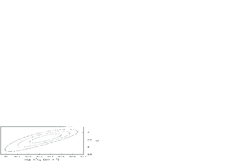
Figure 4: $\Delta\chi^{2}$ confidence region of the standard candle model fit to the union of the differential distribution and the time dilation and energy shifting factors. 1-, 2-, and 3-$\sigma$ are as described in fig. 3.

The standard candle model additionally fits the union of these data sets ($\chi^{2}_{m}=$ 38.2, $\nu=$ 38). The $\Delta\chi^{2}$ confidence region of this joint fit (fig. 4) places strong bounds on both $h^{2}L_{0}$ and $D$: $h^{2}L_{0}=$ 2.3${}^{+0.8}_{-0.7}\times 10^{57}$ ph s^-1 and $D=$ 3.6${}^{+0.3}_{-0.3}$. By eq. 22, this implies that $z_{M}>$ 6.0${}^{+1.5}_{-1.3}$, of which the implications are discussed in §5.

4.2 Power Law Luminosity Distribution Model

The power law model consists of five parameters: $h^{2}\bar{L}$, $D$, $\beta$, $K$, and $z_{M}$, where

$$\bar{L}=L_{m}\left(\frac{1-\beta}{2-\beta}\right)\left(\frac{K^{2-\beta}-1}{K^{1-\beta}-1}\right)$$ (23)

is the mean luminosity of the luminosity distribution, $\phi(L)$. The fifth parameter, $z_{M}$, is again constrained by eq. 22, except with $L_{0}\rightarrow L_{m}$. However, unlike in the standard candle model, $z_{M}$ is not necessarily independent of the data above this limit. For purposes of fitting, we assume that $z_{M}$ is indeed beyond what BATSE observes. The limitations of this assumption are discussed in §5.

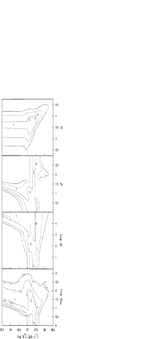
Figure 5: Projected $\Delta\chi^{2}$ confidence regions of the power law model fit to the union of the differential distribution and the time dilation and energy shifting factors. 1-, 2-, and 3-$\sigma$ are as described in fig. 3. Subregions 1 - 4 are described in tab. 1.

The power law model fits the differential distribution ($\chi^{2}_{m}=11.2$, $\nu=$ 14), the time dilation and energy shifting factors ($\chi^{2}_{m}=$ 13.6, $\nu=$ 18), and the union of these data sets ($\chi^{2}_{m}=$ 34.1, $\nu=$ 36). The $\Delta\chi^{2}$ confidence region of the joint fit (fig. 5) places strong bounds on $D$: $D=$ 3.7${}^{+0.4}_{-0.5}$ and for $h^{2}\bar{L}<$ 10⁵⁷ ph s^-1, 3.4 $\mathrel{\hbox{\hbox to0.0pt{\hbox{\lower 4.0pt\hbox{$\sim$}}\hss}\hbox{$<$}}}D\mathrel{\hbox{\hbox to0.0pt{\hbox{\lower 4.0pt\hbox{$\sim$}}\hss}\hbox{$<$}}}$ 3.8 to 1-$\sigma$. This region is additionally divisible into four unique subregions (see tab. 1). Using the terminology of Hakkila et al. (1995, 1996), the luminosity distribution of each subregion is described as $L_{m}$ dominated (independent of $L_{M}$), $L_{M}$ dominated (independent of $L_{m}$), range dominated (dependent upon both $L_{m}$ and $L_{M}$), or similar to a standard candle ($L_{m}\sim L_{M}$). For each subregion, bounds are placed on $\bar{L}$, $\beta$, $K$, and $K_{90}$, where $K_{90}$ is the 90% width of the observed luminosity distribution and is given by (following the convention of Ulmer & Wijers (1995))

$$K_{90}=\frac{L_{95}}{L_{5}},$$ (24)

where $L_{p}$, the “$p$% luminosity” of this distribution, is defined by

$$N_{L<L_{p}}(>F_{m})=\left(\frac{p}{100}\right)N_{L<L_{M}}(>F_{m}).$$ (25)

It is important to note that others (e.g., Horack, Emslie, & Meegan (1994)) define $K_{90}$ differently:

$$K_{90}=\cases{\frac{L_{90}}{L_{m}}&($L_{m}$ dominated)\cr\frac{L_{M}}{L_{10}}&($L_{M}$ dominated)},$$ (26)

which results in reduced values. The former definition is applied here.

5 Conclusions

Assuming no evolution ($D=$ 3), Fenimore & Bloom (1995), Nemiroff et al. (1996), and Horack, Mallozzi, & Koshut (1996) have demonstrated that BATSE’s differential distribution is inconsistent with a time dilation factor of $\sim$ 2 between the peak flux extremes of Norris et al. (1996a, 1996b). This has prompted suggestions that either the bursts’ observed time dilation is largely intrinsic or that strong evolutionary effects are present in the differential distribution. The former explanation, however, is discredited by the degree to which the time dilation and energy shifting measurements are consistent. Hakkila et al. (1996), also assuming no evolution, have demonstrated that the differential distribution alone is incompatible with a standard candle luminosity. These results agree with our results for $D=3$. We additionally determine at what values of $D$ that these incompatibilities disappear: $D=$ 3.6${}^{+0.3}_{-0.3}$ for the standard candle model and $D=$ 3.7${}^{+0.4}_{-0.5}$ for the power law model. For mean luminosities $h^{2}\bar{L}<$ 10⁵⁷ ph s^-1, evolution is even more tightly constrained: 3.4 $\mathrel{\hbox{\hbox to0.0pt{\hbox{\lower 4.0pt\hbox{$\sim$}}\hss}\hbox{$<$}}}D\mathrel{\hbox{\hbox to0.0pt{\hbox{\lower 4.0pt\hbox{$\sim$}}\hss}\hbox{$<$}}}$ 3.8 (to 1-$\sigma$).

Horack, Emslie, & Meegan (1994), Emslie & Horack (1994), Ulmer & Wijers (1995), Hakkila et al. (1995, 1996), and Ulmer, Wijers, & Fenimore (1995) have demonstrated that $K_{90}\mathrel{\hbox{\hbox to0.0pt{\hbox{\lower 4.0pt\hbox{$\sim$}}\hss}\hbox{$<$}}}$ 10 for a variety of galactic halo and cosmological models. When cosmological, these models assume no evolution. However, when $D>$ 3, $K_{90}$ need not be so tightly constrained (Horack, Emslie, & Hartmann 1995, Horack et al. (1996)). We find that for 10⁵⁷ ph s^-1 $\mathrel{\hbox{\hbox to0.0pt{\hbox{\lower 4.0pt\hbox{$\sim$}}\hss}\hbox{$<$}}}h^{2}\bar{L}\mathrel{\hbox{\hbox to0.0pt{\hbox{\lower 4.0pt\hbox{$\sim$}}\hss}\hbox{$<$}}}$ 10^57.5 ph s^-1, $K_{90}$ is only constrained to be less than $\sim 10^{2}$ (see fig. 5). Furthermore, for $h^{2}\bar{L}\mathrel{\hbox{\hbox to0.0pt{\hbox{\lower 4.0pt\hbox{$\sim$}}\hss}\hbox{$<$}}}$ 10⁵⁶ ph s^-1, $K_{90}\mathrel{\hbox{\hbox to0.0pt{\hbox{\lower 4.0pt\hbox{$\sim$}}\hss}\hbox{$>$}}}$ 10. The former result is more conservative than estimates which assume no evolution. The latter is the result of new solutions which do not fit the data for $D=$ 3.

In the standard candle model, the redshift of BATSE’s faintest burst is 6.0${}^{+1.5}_{-1.3}$, which is much greater than that which is measured for galaxies. The power law model, under certain conditions, provides more reasonable estimates. In tab. 2, 1-$\sigma$ bounds are placed on the redshift of BATSE’s faintest burst for three representative luminosities: $L_{10}$, $L_{50}$, and $L_{90}$, where $L_{p}$ is as defined in eq. 25. (For example, $L_{50}$ is the median luminosity of the observed luminosity distribution, and 80% of the observed bursts have luminosities between $L_{10}$ and $L_{90}$.) Defining the redshift $z_{p}$ as the maximum redshift at which bursts of luminosity $L_{p}$ can be detected, we find that 2.9 $\mathrel{\hbox{\hbox to0.0pt{\hbox{\lower 4.0pt\hbox{$\sim$}}\hss}\hbox{$<$}}}z_{50}\mathrel{\hbox{\hbox to0.0pt{\hbox{\lower 4.0pt\hbox{$\sim$}}\hss}\hbox{$<$}}}$ 4.6 for $h^{2}\bar{L}\mathrel{\hbox{\hbox to0.0pt{\hbox{\lower 4.0pt\hbox{$\sim$}}\hss}\hbox{$<$}}}$ 10⁵⁷ ph s^-1 and 4.2 $\mathrel{\hbox{\hbox to0.0pt{\hbox{\lower 4.0pt\hbox{$\sim$}}\hss}\hbox{$<$}}}z_{50}\mathrel{\hbox{\hbox to0.0pt{\hbox{\lower 4.0pt\hbox{$\sim$}}\hss}\hbox{$<$}}}$ 9.4 otherwise. However, $z_{10}\mathrel{\hbox{\hbox to0.0pt{\hbox{\lower 4.0pt\hbox{$\sim$}}\hss}\hbox{$<$}}}$ 4.2 for all mean luminosities and $\mathrel{\hbox{\hbox to0.0pt{\hbox{\lower 4.0pt\hbox{$\sim$}}\hss}\hbox{$<$}}}$ 2.3 for $h^{2}\bar{L}\mathrel{\hbox{\hbox to0.0pt{\hbox{\lower 4.0pt\hbox{$\sim$}}\hss}\hbox{$<$}}}$ 10⁵⁷ ph s^-1. If $L_{p}\mathrel{\hbox{\hbox to0.0pt{\hbox{\lower 4.0pt\hbox{$\sim$}}\hss}\hbox{$>$}}}L_{90}$, the redshift of this burst is again quite large. Consequently, a mean luminosity of $h^{2}\bar{L}\mathrel{\hbox{\hbox to0.0pt{\hbox{\lower 4.0pt\hbox{$\sim$}}\hss}\hbox{$<$}}}$ 10⁵⁷ ph s^-1 coupled with a luminosity for BATSE’s faintest burst of $L_{p}<L_{50}$ is favored.

In conclusion, the results presented in this paper demonstrate that when both the differential distribution and the time dilation and energy shifting factors are fitted to, moderate evolution is required if an Einstein-de Sitter cosmology, a power law spectrum of photon number index -1, no luminosity evolution, and in the case of the power law model, a non-observable maximum burst redshift are assumed. We have additionally demonstrated that under these conditions, the 90% width of the observed luminosity distribution is not necessarily $\mathrel{\hbox{\hbox to0.0pt{\hbox{\lower 4.0pt\hbox{$\sim$}}\hss}\hbox{$<$}}}$ 10, as appears to be the case if no evolution is assumed. Finally, redshift considerations indicate that if the redshifts of the faintest bursts are to be compatible with that which is currently known about galaxies, the standard candle model is unacceptable and for the power law model, a mean burst luminosity $h^{2}\bar{L}\mathrel{\hbox{\hbox to0.0pt{\hbox{\lower 4.0pt\hbox{$\sim$}}\hss}\hbox{$<$}}}$ 10⁵⁷ ph cm^-2 s^-1 is favored.

Table 1: Power Law Model $\Delta\chi^{2}$ Confidence Subregions

Subregion	$\phi(L)$	$\bar{L}$	$\beta$	$K$	$K_{90}$
1	$L_{M}$ dominated	$\mathrel{\hbox{\hbox to0.0pt{\hbox{\lower 4.0pt\hbox{$\sim$}}\hss}\hbox{$<$}}}L_{0}$	unbounded	$\mathrel{\hbox{\hbox to0.0pt{\hbox{\lower 4.0pt\hbox{$\sim$}}\hss}\hbox{$>$}}}$ 103	$\mathrel{\hbox{\hbox to0.0pt{\hbox{\lower 4.0pt\hbox{$\sim$}}\hss}\hbox{$>$}}}$ 100.5
2	range dominated	$\sim L_{0}$	$\mathrel{\hbox{\hbox to0.0pt{\hbox{\lower 4.0pt\hbox{$\sim$}}\hss}\hbox{$<$}}}$ 1.5	$\mathrel{\hbox{\hbox to0.0pt{\hbox{\lower 4.0pt\hbox{$\sim$}}\hss}\hbox{$<$}}}$ 103	$\mathrel{\hbox{\hbox to0.0pt{\hbox{\lower 4.0pt\hbox{$\sim$}}\hss}\hbox{$<$}}}$ 102
3	standard candle	$\sim L_{0}$	unbounded	$\sim$ 1	$\sim$ 1
4	$L_{m}$ dominated	$\sim L_{0}$	$\mathrel{\hbox{\hbox to0.0pt{\hbox{\lower 4.0pt\hbox{$\sim$}}\hss}\hbox{$>$}}}$ 2.5	$\mathrel{\hbox{\hbox to0.0pt{\hbox{\lower 4.0pt\hbox{$\sim$}}\hss}\hbox{$>$}}}$ 102.5	$\mathrel{\hbox{\hbox to0.0pt{\hbox{\lower 4.0pt\hbox{$\sim$}}\hss}\hbox{$<$}}}$ 10

Table 2: Power Law Model Redshift of BATES’s Faintest Burst

$L_{p}$	$h^{2}\bar{L}\mathrel{\hbox{\hbox to0.0pt{\hbox{\lower 4.0pt\hbox{$\sim$}}\hss}\hbox{$<$}}}$ 1057 ph s-1	$h^{2}\bar{L}\mathrel{\hbox{\hbox to0.0pt{\hbox{\lower 4.0pt\hbox{$\sim$}}\hss}\hbox{$>$}}}$ 1057 ph s-1
$L_{10}$	1.0 $\mathrel{\hbox{\hbox to0.0pt{\hbox{\lower 4.0pt\hbox{$\sim$}}\hss}\hbox{$<$}}}z_{10}\mathrel{\hbox{\hbox to0.0pt{\hbox{\lower 4.0pt\hbox{$\sim$}}\hss}\hbox{$<$}}}$ 2.3	1.2 $\mathrel{\hbox{\hbox to0.0pt{\hbox{\lower 4.0pt\hbox{$\sim$}}\hss}\hbox{$<$}}}z_{10}\mathrel{\hbox{\hbox to0.0pt{\hbox{\lower 4.0pt\hbox{$\sim$}}\hss}\hbox{$<$}}}$ 4.2
$L_{50}$	2.9 $\mathrel{\hbox{\hbox to0.0pt{\hbox{\lower 4.0pt\hbox{$\sim$}}\hss}\hbox{$<$}}}z_{50}\mathrel{\hbox{\hbox to0.0pt{\hbox{\lower 4.0pt\hbox{$\sim$}}\hss}\hbox{$<$}}}$ 4.6	4.2 $\mathrel{\hbox{\hbox to0.0pt{\hbox{\lower 4.0pt\hbox{$\sim$}}\hss}\hbox{$<$}}}z_{50}\mathrel{\hbox{\hbox to0.0pt{\hbox{\lower 4.0pt\hbox{$\sim$}}\hss}\hbox{$<$}}}$ 9.4
$L_{90}$	5.1 $\mathrel{\hbox{\hbox to0.0pt{\hbox{\lower 4.0pt\hbox{$\sim$}}\hss}\hbox{$<$}}}z_{90}\mathrel{\hbox{\hbox to0.0pt{\hbox{\lower 4.0pt\hbox{$\sim$}}\hss}\hbox{$<$}}}$ 6.1	5.3 $\mathrel{\hbox{\hbox to0.0pt{\hbox{\lower 4.0pt\hbox{$\sim$}}\hss}\hbox{$<$}}}z_{90}\mathrel{\hbox{\hbox to0.0pt{\hbox{\lower 4.0pt\hbox{$\sim$}}\hss}\hbox{$<$}}}$ 13.1

References

- Band (1993) Band, D. 1993, ApJ, 413, 281
- Bloom, Fenimore, & in ’t Zand (1996) Bloom, J. S., Fenimore, E. E., & in ’t Zand, J. 1996, in Proc. of the 3rd Huntsville Gamma Ray Burst Symposium, AIP, in press
- Briggs et al. (1996) Briggs, M. S., et al. 1996, ApJ, 459, 40
- Davis (1995) Davis, S. P. 1995, Ph.D. thesis, The Catholic Univ. of America
- Emslie, & Horack (1994) Emslie, A. G., & Horack, J. M. 1994, ApJ, 435, 16
- Fenimore & Bloom (1995) Fenimore, E. E., & Bloom, J. S. 1995, ApJ, 453, 25
- Fenimore et al. (1993) Fenimore, E. E., et al. 1993, Nature, 366, 40
- Fenimore et al. (1995) Fenimore, E. E., et al. 1995, ApJ, 448, L101
- Hakkila et al. (1995) Hakkila, J., et al. 1995, ApJ, 454, 134
- Hakkila et al. (1996) Hakkila, J., et al. 1996, ApJ, 462, 125
- Horack, Emslie, & Hartmann (1995) Horack, J. M., Emslie, A. G., & Hartmann, D. H. 1995, ApJ, 447, 474