Microwave Background Constraints on Cosmological Parameters

Abstract

We use a high-accuracy computational code to investigate the precision with which cosmological parameters could be reconstructed by future cosmic microwave background experiments. We focus on the two planned satellite missions: MAP and Planck. We identify several parameter combinations that could be determined with a few percent accuracy with the two missions, as well as some degeneracies among the parameters that cannot be accurately resolved with the temperature data alone. These degeneracies can be broken by other astronomical measurements. Polarization measurements can significantly enhance the science return of both missions by allowing a more accurate determination of some cosmological parameters, by enabling the detection of gravity waves and by probing the ionization history of the universe. We also address the question of how gaussian the likelihood function is around the maximum and whether gravitational lensing changes the constraints.

1 Introduction

Measurements of cosmic microwave background (CMB) anisotropies have already revolutionized cosmology by providing insight into the physical conditions of the universe only three hundred thousand years after the Big Bang. The first year COBE data (Smoot et al. (1992)) determined the amplitude of the large angular scale CMB power spectrum with an accuracy of 10% and the spectral slope with an accuracy of $0.3$. With the 4-year COBE data (Bennett et al. (1996)), these constraints became the tightest cosmological constraints available. Recent results from over a dozen balloon and ground based experiments are beginning to explore the anisotropies on smaller angular scales, which will help to constrain other cosmological parameters as well. The future looks even more promising: there are now two planned satellite missions, MAP and Planck. Both missions will provide a map of the whole sky with a fraction of a degree angular resolution and sufficient signal to noise to reconstruct the underlying power spectrum with an unprecedented accuracy.

A wonderful synergy is taking place in the study of the cosmic background radiation: theorists are able to make very accurate predictions of CMB anisotropies (Bond & Efstathiou 1987; Hu et al. 1995; Bond 1996; Seljak & Zaldarriaga 1996), while experimentalists are rapidly improving our ability to measure these anisotropies. If the results are consistent with structure formation from adiabatic curvature fluctuations (as predicted by inflation), then they can be used to accurately determine a number of cosmological parameters. If the measurements are not consistent with any of the standard models, cosmologists will need to rethink ideas about the origin of structure formation in the universe. In either case, CMB will provide information about fundamental properties of our universe.

It has long been recognized that the microwave sky is sensitive to many cosmological parameters, so that a high resolution map may lead to their accurate determination (Bond et al. (1994); Spergel (1994); Knox (1995); Jungman et al. (1996); Bond et al. (1997)). The properties of the microwave background fluctuations are sensitive to the geometry of the universe, the baryon-to-photon ratio, the matter-to-photon ratio, the Hubble constant, the cosmological constant, and the optical depth due to reionization in the universe. A stochastic background of gravitational waves also leaves an imprint on the CMB and their amplitude and slope may be extracted from the observations. In addition, massive neutrinos and a change in the slope of the primordial spectrum also lead to potentially observable features.

Previous calculations trying to determine how well the various parameters could be constrained were based on approximate methods for computing the CMB spectra (Jungman et al. (1996)). These approximations have an accuracy of several percent, which suffices for the analysis of the present-day data. However, the precision of the future missions will be so high that the use of such approximations will not be sufficient for an accurate determination of the parameters. Although high accuracy calculations are not needed at present to analyze the observations, they are needed to determine how accurately cosmological parameters can be extracted from a given experiment. This is important not only for illustrative purposes but may also help to guide the experimentalists in the design of the detectors. One may for example address the question of how much improvement one can expect by increasing the angular resolution of an experiment (and by doing so increasing the risk of systematic errors) to decide whether this improvement is worth the additional risk. Another question of current interest is whether it is worth sacrificing some sensitivity in the temperature maps to gain additional information from the polarization of the microwave background. When addressing these questions, the shortcomings of approximations become particularly problematic. The sensitivity to a certain parameter depends on the shape of the likelihood function around the maximum, which in the simplest approach used so far is calculated by differentiating the spectrum with respect to the relevant parameter. This differentiation strongly amplifies any numerical inaccuracies: this almost always leads to an unphysical breaking of degeneracies among parameters and misleadingly optimistic results.

Previous analysis of CMB sensitivity to cosmological parameters used only temperature information. However, CMB experiments can measure not just the temperature fluctuations, but also even weaker variations in the polarization of the microwave sky. Instead of one power spectrum, one can measure up to four and so increase the amount of information in the two-point correlators (Seljak 1996b ; Zaldarriaga and Seljak (1997), Kamionkowski, Kosowsky & Stebbins 1997). Polarization can provide particularly useful information regarding the ionization history of the universe (Zaldarriaga (1996)) and the presence of a tensor contribution (Seljak & Zaldarriaga (1997); Kamionkowski et al. (1997)). Because these parameters are partially degenerate with others, any improvement in their determination leads to a better reconstruction of other parameters as well. The two proposed satellite missions are currently investigating the possibility of adding or improving their ability to measure polarization, so it is particularly interesting to address the question of improvement in the parameter estimation that results from polarization.

The purpose of this paper is to re-examine the determination of cosmological parameters by CMB experiments in light of the issues raised above. It is particularly timely to perform such an analysis now, when the satellite mission parameters are roughly defined. We use the best current mission parameters in the calculations and hope that our study provides a useful guide for mission optimization. As in previous work (Jungman et al. (1996)), we use the Fisher information matrix to answer the question of how accurately parameters can be extracted from the CMB data. This approach requires a fast and accurate method for calculating the spectra and we use the CMBFAST package (Seljak & Zaldarriaga (1996)) with an accuracy of about 1%. We test the Fisher information method by performing a more general exploration of the shape of the likelihood function around its maximum and find that this method is sufficiently accurate for the present purpose.

The outline of this paper is the following: in §2, we present the methods used, reviewing the calculation of theoretical spectra and the statistical methods to address the question of sensitivity to cosmological parameters. In §3, we investigate the parameter sensitivity that could be obtained using temperature information only and in §4, we repeat this analysis using both temperature and polarization information. In §5, we explore the accuracy of the Fisher method by performing a more general type of analysis and investigate the effects of prior information in the accuracy of the reconstruction. We present our conclusions in §6.

2 Methods

In this section, we review the methods used to calculate the constraints on different cosmological parameters that could be obtained by the future CMB satellite experiments. We start by reviewing the statistics of CMB anisotropies in §2.1, where we also present the equations that need to be solved to compute the theoretical prediction for the spectra in the integral approach developed by Seljak & Zaldarriaga (1996a). In §2.2, we discuss the Fisher information matrix approach, as well as the more general method of exploring the shape of the likelihood function around the minimum.

2.1 Statistics of the microwave background

The CMB radiation field is characterized by a $2\times 2$ intensity tensor $I_{ij}$. The Stokes parameters $Q$ and $U$ are defined as $Q=(I_{11}-I_{22})/4$ and $U=I_{12}/2$, while the temperature anisotropy is given by $T=(I_{11}+I_{22})/4$. In principle the fourth Stokes parameter $V$ that describes circular polarization would also be needed, but in standard cosmological models it can be ignored because it cannot be generated through the process of Thomson scattering, the only relevant interaction process. While the temperature is a scalar quantity that can naturally be expanded in spherical harmonics, $(Q\pm iU)$ should be expanded using spin weight $\pm\ 2$ harmonics, (Zaldarriaga and Seljak (1997); Goldberg et al. (1967); Gelfand et al. (1963), see also Kamionkowski et al. (1997) for an alternative expansion)

$$T(\hat{\hbox{\boldmath{$n$}}}) = \sum_{lm}a_{T,lm}Y_{lm}(\hat{\hbox{\boldmath{$n$}}})$$

$$(Q+iU)(\hat{\hbox{\boldmath{$n$}}}) = \sum_{lm}a_{2,lm}\;{}_{2}Y_{lm}(\hat{\hbox{\boldmath{$n$}}})$$

$$(Q-iU)(\hat{\hbox{\boldmath{$n$}}}) = \sum_{lm}a_{-2,lm}\;{}_{-2}Y_{lm}(\hat{\hbox{\boldmath{$n$}}}).$$ (1)

The expansion coefficients satisfy $a_{-2,lm}^{*}=a_{2,l-m}$ and $a_{T,lm}^{*}=a_{T,l-m}$. Instead of $a_{2,lm}$ and $a_{-2,lm}$ it is convenient to introduce their even and odd parity linear combinations (Newman & Penrose (1966))

$$a_{E,lm}=-(a_{2,lm}+a_{-2,lm})/2$$

$$a_{B,lm}=i(a_{2,lm}-a_{-2,lm})/2.$$ (2)

These two combinations behave differently under parity transformation: while $E$ remains unchanged $B$ changes sign, in analogy with electric and magnetic fields.

The statistics of the CMB are characterized by the power spectra of these variables together with their cross-correlations. Only the cross correlation between $E$ and $T$ is expected to be non-zero, as $B$ has the opposite parity to both $E$ and $T$. The power spectra are defined as the rotationally invariant quantities

$$C_{Tl} = {1\over 2l+1}\sum_{m}\langle a_{T,lm}^{*}a_{T,lm}\rangle$$

$$C_{El} = {1\over 2l+1}\sum_{m}\langle a_{E,lm}^{*}a_{E,lm}\rangle$$

$$C_{Bl} = {1\over 2l+1}\sum_{m}\langle a_{B,lm}^{*}a_{B,lm}\rangle$$

$$C_{Cl} = {1\over 2l+1}\sum_{m}\langle a_{T,lm}^{*}a_{E,lm}\rangle.$$ (3)

The four spectra above contain all the information on a given theoretical model, at least for the class of models described by gaussian random fields. To test the sensitivity of the microwave background to a certain cosmological parameter, we have to compute the theoretical predictions for these spectra. This can be achieved by evolving the system of Einstein, fluid, and Boltzmann equations from an early epoch to the present. The solution for the spectra above can be written as a line-of-sight integral over sources generated by these initial perturbations (Seljak & Zaldarriaga (1996)). For density perturbations (scalar modes), the power spectra for $T$ and $E$ and their cross-correlation are given by (the odd parity mode $B$ being zero in this case),

$$C_{T,El}^{(S)} = (4\pi)^{2}\int k^{2}dkP_{\phi}(k)\Big{[}\Delta^{(S)}_{T,El}(k)\Big{]}^{2}$$

$$C_{Cl}^{(S)} = (4\pi)^{2}\int k^{2}dkP_{\phi}(k)\Delta^{(S)}_{Tl}(k)\Delta^{(S)}_{El}(k),$$ (4)

The source terms can be written as an integral over conformal time (Seljak & Zaldarriaga (1996), Zaldarriaga and Seljak (1997)),

$$\Delta^{(S)}_{Tl}(k) = \int_{0}^{\tau_{0}}d\tau S^{(S)}_{T}(k,\tau)j_{l}(x)$$

$$\Delta^{(S)}_{El}(k) = \sqrt{(l+2)!\over(l-2)!}\int_{0}^{\tau_{0}}d\tau S^{(S)}_{E}(k,\tau)j_{l}(x)$$

$$S_{T}^{(S)}(k,\tau) = g\left(\Delta_{T,0}+2\ddot{\alpha}+{\dot{v_{b}}\over k}+{\Pi\over 4}+{3\ddot{\Pi}\over 4k^{2}}\right)$$

$$+ e^{-\kappa}(\dot{\eta}+\ddot{\alpha})+\dot{g}\left({v_{b}\over k}+{3\dot{\Pi}\over 4k^{2}}\right)+{3\ddot{g}\Pi\over 4k^{2}}$$

$$S^{(S)}_{E}(k\tau) = {3g(\tau)\Pi(\tau,k)\over 4x^{2}},$$

$$\Pi = \Delta_{T2}^{(S)}+\Delta_{P2}^{(S)}+\Delta_{P0}^{(S)},$$ (5)

where $x=k(\tau_{0}-\tau)$, $\tau_{0}$ is the present time and $\alpha=(\dot{h}+6\dot{\eta})/2k^{2}$. The derivatives are taken with respect to the conformal time $\tau$. The differential optical depth for Thomson scattering is denoted as $\dot{\kappa}=an_{e}x_{e}\sigma_{T}$, where $a(\tau)$ is the expansion factor normalized to unity today, $n_{e}$ is the electron density, $x_{e}$ is the ionization fraction and $\sigma_{T}$ is the Thomson cross section. The total optical depth at time $\tau$ is obtained by integrating $\dot{\kappa}$, $\kappa(\tau)=\int_{\tau}^{\tau_{0}}\dot{\kappa}(\tau)d\tau$. We also introduced the visibility function $g(\tau)=\dot{\kappa}\ {\rm exp}(-\kappa)$. Its peak defines the epoch of recombination, which gives the dominant contribution to the CMB anisotropies. The sources in these equations involve the multipole moments of temperature and polarization, which are defined as $\Delta(k,\mu)=\sum_{l}(2l+1)(-i)^{l}\Delta_{l}(k)P_{l}(\mu)$, where $P_{l}(\mu)$ is the Legendre polynomial of order $l$. Temperature anisotropies have additional sources in the metric perturbations $h$ and $\eta$ and in the baryon velocity term $v_{b}$ (Bond & Efstathiou 1994; 1987; Ma & Bertschinger 1996). The expressions above are only valid in the flat space limit; see Zaldarriaga, Seljak & Bertschinger (1997) for the appropriate generalization to open geometries.

The solution for gravity waves can be similarly written as (Zaldarriaga and Seljak (1997))

$$\Delta_{Tl}^{(T)} = \sqrt{(l+2)!\over(l-2)!}\int_{0}^{\tau_{0}}d\tau S_{T}^{(T)}(k,\tau){j_{l}(x)\over x^{2}}$$

$$\Delta_{E,Bl}^{(T)} = \int_{0}^{\tau_{0}}d\tau S_{E,B}^{(T)}(k,\tau)j_{l}(x)$$

$$S_{T}^{(T)}(k,\tau) = -\dot{h}e^{-\kappa}+g\Psi$$

$$S_{E}^{(T)}(k,\tau) = -g\left(\Psi-{\ddot{\Psi}\over k^{2}}+{2\Psi\over x^{2}}-{\dot{\Psi}\over kx}\right)+\dot{g}\left({2\dot{\Psi}\over k^{2}}+{4\Psi\over kx}\right)+2\ddot{g}{\Psi\over k^{2}}$$

$$S_{B}^{(T)}(k,\tau) = g\left({4\Psi\over x}+{2\dot{\Psi}\over k}\right)+2\dot{g}{\Psi\over k}$$ (6)

$$\Psi \equiv\Biggl{[}{1\over 10}\tilde{\Delta}_{T0}^{(T)}+{1\over 7}\tilde{\Delta}_{T2}^{(T)}+{3\over 70}\tilde{\Delta}_{T4}^{(T)}-{3\over 5}\tilde{\Delta}_{P0}^{(T)}+{6\over 7}\tilde{\Delta}_{P2}^{(T)}-{3\over 70}\tilde{\Delta}_{P4}^{(T)}\Biggr{]},$$

where the power spectra are obtained by integrating the contributions over all the wavevectors as in equation (4). Note that in the case of tensor polarization perturbations both $E$ and $B$ are present and can be measured separately. Inflationary models predict no vector component and we do not include a vector component in our analysis.

2.2 The Fisher information matrix

The Fisher information matrix is a measure of the width and shape of the likelihood function around its maximum. Its elements are defined as expectation values of the second derivative of a logarithm of the likelihood function with respect to the corresponding pair of parameters. It can be used to estimate the accuracy with which the parameters in the cosmological model could be reconstructed using the CMB data (Jungman et al. (1996), Tegmark et al. (1996)). If only temperature information is given then for each $l$ a derivative of the temperature spectrum $C_{Tl}$ with respect to the parameter under consideration is computed and this information is then summed over all $l$ weighted by ${\rm Cov}^{-1}(\hat{C}_{Tl}^{2})$. In the more general case implemented here, we have a vector of four derivatives and the weighting is given by the inverse of the covariance matrix,

$$\alpha_{ij}=\sum_{l}\sum_{X,Y}{\partial C_{Xl}\over\partial s_{i}}{\rm Cov}^{-1}(\hat{C}_{Xl},\hat{C}_{Yl}){\partial C_{Yl}\over\partial s_{j}}.$$ (7)

Here $\alpha_{ij}$ is the Fisher information matrix, ${\rm Cov}^{-1}$ is the inverse of the covariance matrix, $s_{i}$ are the cosmological parameters one would like to estimate and $X,Y$ stands for $T,E,B,C$. For each $l$, one has to invert the covariance matrix and sum over $X$ and $Y$. The derivatives were calculated by finite differences and the step was usually taken to be about $5\%$ of the value of each parameter. We explored the dependence of our results on this choice and found that the effect is less than $10\%$. This indicates that the likelihood surface is approximately gaussian. Further tests of this assumption are discussed in §5.

The full covariance matrix between the power spectra estimators was presented in Seljak 1996b , Zaldarriaga and Seljak (1997) and Kamionkowski et al. (1997). The diagonal terms are given by

$${\rm Cov}(\hat{C}_{Tl}^{2}) = {2\over(2l+1)f_{sky}}({C}_{Tl}+w_{T}^{-1}B_{l}^{-2})^{2}$$

$${\rm Cov}(\hat{C}_{El}^{2}) = {2\over(2l+1)f_{sky}}({C}_{El}+w_{P}^{-1}B_{l}^{-2})^{2}$$

$${\rm Cov}(\hat{C}_{Bl}^{2}) = {2\over(2l+1)f_{sky}}({C}_{Bl}+w_{P}^{-1}B_{l}^{-2})^{2}$$

$${\rm Cov}(\hat{C}_{Cl}^{2}) = {1\over(2l+1)f_{sky}}\left[{C}_{Cl}^{2}+({C}_{Tl}+w_{T}^{-1}B_{l}^{-2})({C}_{El}+w_{P}^{-1}B_{l}^{-2})\right],$$ (8)

while the non-zero off diagonal terms are

$${\rm Cov}(\hat{C}_{Tl}\hat{C}_{El}) = {2\over(2l+1)f_{sky}}{C}_{Cl}^{2}$$

$${\rm Cov}(\hat{C}_{Tl}\hat{C}_{Cl}) = {2\over(2l+1)f_{sky}}{C}_{Cl}({C}_{Tl}+w_{T}^{-1}B_{l}^{-2})$$

$${\rm Cov}(\hat{C}_{El}\hat{C}_{Cl}) = {2\over(2l+1)f_{sky}}{C}_{Cl}({C}_{El}+w_{P}^{-1}B_{l}^{-2}).$$ (9)

We have defined $w_{(T,P)}^{-1}=4\pi\sigma_{(T,P)}^{2}/N_{pix}$ where $\sigma_{T}$ and $\sigma_{P}$ are noise per pixel in the temperature and either $Q$ or $U$ polarization measurements (they are assumed equal) and $N_{pix}$ is the number of pixels. We will also assume that noise is uncorrelated between different pixels and between different polarization components $Q$ and $U$. This is only the simplest possible choice and more complicated noise correlations arise if all the components are obtained from a single set of observations. If both temperature and polarization are obtained from the same experiment by adding and differenciating the two polarization states, then $\sigma_{T}^{2}=\sigma_{P}^{2}/2$ and noise in temperature is uncorrelated with noise in polarization components. The window function $B_{l}^{-2}$ accounts for the beam smearing and in the gaussian approximation is given by $B_{l}^{-2}=e^{l^{2}\sigma_{b}^{2}}$, with $\sigma_{b}$ measuring the width of the beam. We introduced $f_{sky}$ as the fraction of the sky that can be used in the analysis. In this paper we assume $f_{sky}=0.8$. It should be noted that equations (8) and (9) are valid in the limit of uniform sky coverage.

Both satellite missions will measure in several frequency channels with different angular resolutions: we combine them using $w_{(T,P)}=\sum w_{(T,P)}^{c}$, where subscript $c$ refers to each channel component. For MAP mission we adopt a noise level $w_{T}^{-1}=(0.11\mu K)^{2}$ and $w_{P}^{-1}=(0.15\mu K)^{2}$ for the combined noise of the three highest frequency channels with conservatively updated MAP beam sizes: $0.53^{\circ}$, $0.35^{\circ}$ and $0.25^{\circ}$. These beam sizes are smaller than those in the MAP proposal and represent improved estimates of MAP’s resolution. The most recent estimates of MAP’s beam sizes are even smaller: $0.47^{\circ}$, $0.35^{\circ}$ and $0.21^{\circ}$ For Planck, we assume $w_{T}^{-1}=(0.011\mu K)^{2}$ and $w_{P}^{-1}=(0.025\mu K)^{2}$, and combine the $140$ GHz and $210$ GHz bolometer channels. For Planck’s polarization sensitivity, we assume a proposed design in which eight out of twelve receivers in each channel have polarizers (Efstathiou 1996). The angular resolution at these frequencies is $0.16^{\circ}$ and $0.12^{\circ}$ FWHM. We also explore the possible science return from an enhanced bolometer system that achieves polarization sensitivity of $w_{P}^{-1}=(0.015\mu K)^{2}$.

In our analysis, we are assuming that foregrounds can be subtracted from the data to the required accuracy. Previous studies of temperature anisotropies have shown that this is not an overly optimistic assumption at least on large angular scales (e.g., Tegmark & Efstathiou (1996)). On smaller scales, point source removal as well as secondary processes may make extracting the signal more problematic. This would mostly affect our results on Planck, which has enough angular resolution to measure features in the spectrum to $l\sim 3000$. For this reason, we compared the results by changing the maximum $l$ from $3000$ to $1500$. We find that they change by less than $30\%$, so that the conclusions we find should be quite robust. Foregrounds for polarization have not been studied in detail yet. Given that there are fewer foreground sources of polarization and that polarization fractions in CMB and foregrounds are comparable, we will make the optimistic assumption that the foregrounds can be subtracted from the polarization data with sufficient accuracy as well. However, as we will show, most of the additional information from polarization comes from very large angular scales, where the predicted signal is very small. Thus, one should take our results on polarization as preliminary, until a careful analysis of foreground subtraction in polarization shows at what level can polarization signal be extracted.

The inverse of the Fisher matrix, $\alpha^{-1}$, is an estimate of the covariance matrix between parameters and $\sqrt{(\alpha^{-1})_{ii}}$ approximates the standard error in the estimate of the parameter $s_{i}$. This is the lower limit because Cramér-Rao inequality guarantees that for an unbiased estimator the variance on i-th parameter has to be equal to or larger than $\sqrt{(\alpha^{-1})_{ii}}$. In addition to the diagonal elements of $\alpha^{-1}$, we will also use $2\times 2$ submatrices of $\alpha^{-1}$ to analyze the covariance between various pairs of parameters. The Fisher matrix depends not only on the experiment under consideration, but also on the assumed family of models and on the number of parameters that are being extracted from the data. To highlight this dependence and to assess how the errors on the parameters depend on these choices we will vary their number and consider several different underlying models.

2.3 Minimization

The Fisher information matrix approach assumes that the shape of the likelihood function around the maximum can be approximated by a gaussian. In this section, we drop this assumption and explore directly the shape of the likelihood function. We use the PORT optimization routines (Gay (1990)) to explore one direction in parameter space at a time by fixing one parameter to a given value and allowing the minimization routine to explore the rest of parameter space to find the minimum of $\chi^{2}=\sum_{l}\sum_{X,Y}(C_{Xl}-C_{Xl}^{*}){\rm Cov}^{-1}(\hat{C}_{Xl}\hat{C}_{Yl})(C_{Yl}-{C}_{Yl}^{*})$, where $C_{Xl}^{*}$ denotes the underlying spectrum. The value of $\chi^{2}$ as a function of this parameter can be compared directly with the Fisher matrix prediction, $\Delta\chi^{2}=(s_{i}-s_{i}^{*})^{2}/(\alpha^{-1})_{ii}$, where $s_{i}^{*}$ is the value of the parameter in the underlying model. This comparison tests not only the shape of the likelihood function around the maximum but also the numerical inaccuracies resulting from differentiating the spectrum with respect to the relevant parameter. The minimization method is also useful for finding explicit examples of degenerate models, models with different underlying parameters but almost indistinguishable spectra.

The additional advantage of the minimization approach is that one can easily impose various prior information on the data in the form of constraints or inequalities. Some of these priors may reflect theoretical prejudice on the part of the person performing the analysis, while others are likely to be less controversial: for example, the requirement that matter density, baryon density and optical depth are all positive. One might also be interested in incorporating priors into the estimation to take other astrophysical information into account, e.g., the limits on the Hubble constant or $\Omega_{m}$ from the local measurements. Such additional information can help to break some of the degeneracies present in the CMB data, as discussed in §3. Note that prior information on the parameters can also be incorporated into the Fisher matrix analysis, but in its simplest formulation only in the form of gaussian constraints and not in the form of inequalities.

The main disadvantage of this more general analysis is the computational cost. At each step the minimization routine has to compute derivatives with respect to all the parameters to find the direction in parameter space towards the minimum. If the initial model is sufficiently close to the minimum, then the code typically requires 5-10 steps to find it and to sample the likelihood shape this has to be repeated for several values of the parameter in question (and also for several parameters). This computational cost is significantly higher than in the Fisher matrix approach, where the derivatives with respect to each parameter need to be computed only once.

3 Constraints from temperature data

In this section, we investigate how measurements of the CMB temperature anisotropies alone can constrain different cosmological parameters. The models studied here are approximately normalized to COBE, which sets the level of signal to noise for a given experiment.

We will start with models in a six-dimensional parameter space $\hbox{\boldmath{$s$}}_{6}=(C_{2}^{(S)},h,\Omega_{\Lambda},\Omega_{b},\tau_{ri},n_{s})$, where the parameters are respectively, the amplitude of the power spectrum for scalar perturbations at $l=2$ in units of $\mu K^{2}$, the Hubble constant in units of 100 km/s/Mpc, the cosmological constant and baryon density in units of critical density, the reionization optical depth and the slope of primordial density spectrum. In models with a non zero optical depth, we assume that the universe is instantaneously and fully reionized, so that the ionization fraction is 0 before redshift of reionization $z_{ri}$ and 1 afterwards. We limit to this simple case because only the total optical depth $\tau_{ri}$ can be usefully constrained without polarization information. We discuss the more general case when we discuss polarization below.

The underlying model is standard CDM $\hbox{\boldmath{$s$}}_{6}=(796,0.5,0,0.05,0.05,1.0)$. Our base model has an optical depth of $0.05$, corresponding to the epoch of reionization at $z_{ri}\approx 13$. Models include gravity waves, fixing the tensor amplitude using the consistency relation predicted by inflation $T/S=-7n_{T}$ and assuming a relation between the scalar and tensor spectral slopes $n_{T}=n_{s}-1$ for $n_{s}<1$ and $n_{T}=0$ otherwise, which is predicted by the simplest models of inflation. The results for MAP are summarized in table 1. It is important to keep in mind that the parameters are highly correlated. By investigating confidence contour plots in planes across the parameter space, one can identify combinations of parameters that can be more accurately determined. Previous analytical work (Seljak (1994); Hu & Sugiyama (1995)) showed that the physics of the acoustic oscillations is mainly determined by two parameters, $\Omega_{b}h^{2}$ and $\Omega_{m}h^{2}$, where $\Omega_{m}$ is the density of matter in units of critical density. There is an approximately flat direction in the three dimensional space of $h$, $\Omega_{b}$ and $\Omega_{m}$: for example, one can change $\Omega_{m}$ and adjust $h$ and $\Omega_{b}$ to keep $\Omega_{b}h^{2}$ and $\Omega_{m}h^{2}$ constant, which will not change the pattern of acoustic oscillations. This degeneracy can be broken in two ways. On large scales, the decay of the gravitational potential at late times in $\Omega_{m}\neq 1$ models (the so called late time integrated Sachs-Wolfe or ISW term) produces an additional component in the microwave anisotropy power spectrum, which depends only on $\Omega_{\Lambda}$ (Kofman & Starobinsky (1985)). Because the cosmic variance (finite number of independent multipole moments) is large for small $l$, this effect cannot completely break the degeneracy. The second way is through the change in the angular size of the acoustic horizon at recombination, which shifts all the features in the spectrum by a multiplicative factor. Around $\Omega_{m}=1$, this shift is a rather weak function of $\Omega_{m}$ and scales approximately as $\Omega_{m}^{-0.1}$, leading to almost no effect at low $l$, but is increasingly more important towards higher $l$. MAP is sensitive to multipole moments up to $l\sim 800$, where this effect is small. Consequently MAP’s ability to determine the cosmological constant will mostly come from large scales and thus will be limited by the large cosmic variance. Planck has a higher angular resolution and significantly lower noise, so it is sensitive to the change in the angular size of the horizon. Because of this Planck can break the parameter degeneracy and determine the cosmological constant to a high precision, as shown in table 2.

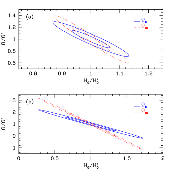
Figure 1: MAP confidence contours (68% and 95%) for models in the six parameter space (a) and seven parameter space with $T/S$ added as a free parameter (b). Parameters are normalized to their value in the underlying model denoted with an asterisk.

Figure 1a shows the confidence contours in the $\Omega_{m}-h$ and $\Omega_{b}-h$ planes. The error ellipses are significantly elongated along the lines $\Delta\Omega_{b}/\Omega_{b}+2.1\Delta h/h=0$ and $\Delta\Omega_{m}/\Omega_{m}+3.0\Delta h/h=0$. The combinations $\Omega_{b}h^{2.1}$ and $\Omega_{m}h^{3}$ are thus better determined than the parameters $\Omega_{m}$, $\Omega_{b}$ and $h$ themselves, both to about 3% for MAP. It is interesting to note that it is $\Omega_{m}h^{3}$ rather than $\Omega_{m}h^{2}$ that is most accurately determined, which reflects the fact that ISW tends to break the degeneracy discussed above. However, because the ISW effect itself can be mimicked by a tilt in the spectral index the degeneracy remains, but is shifted to a different combination of parameters. One sigma standard errors on the two physically motivated parameters are $\Delta(\Omega_{b}h^{2})/\Omega_{b}h^{2}\approx 3\%$ and $\Delta(\Omega_{m}h^{2})/\Omega_{m}h^{2}\approx 5\%$. The fact that there is a certain degree of degeneracy between the parameters has already been noted in previous work (e.g., Bond et al. (1994)).

Another approximate degeneracy present in the temperature spectra is between the reionization optical depth $\tau_{ri}$ and amplitude $C_{2}^{(S)}$. Reionization uniformly suppresses the anisotropies from recombination by $e^{-\tau_{ri}}$. On large angular scales, new anisotropies are generated during reionization by the modes that have not yet entered the horizon. The new anisotropies compensate the $e^{-\tau_{ri}}$ suppression, so that there is no suppression of anisotropies on COBE scales. On small scales, the modes that have entered the horizon have wavelengths small compared to the width of the new visibility function and so are suppressed because of cancellations between positive and negative contributions along the line of sight and become negligible. The net result is that on small scales the spectrum is suppressed by $e^{-2\tau_{ri}}$ compared to the large scales. To break the degeneracy between $C_{2}^{(S)}$ and $\tau_{ri}$ one has to be able to measure the amplitude of the anisotropies on both large and small scales and this is again limited on large scales by cosmic variance. Hence one cannot accurately determine the two parameters separately, while their combination $C_{2}e^{-2\tau_{ri}}$ is much better constrained. Figure 2 shows that indeed the error ellipsoid is very elongated in the direction $\Delta C_{2}/C_{2}-0.1\Delta\tau_{ri}/\tau_{ri}=0$, which corresponds to the above combination for $\tau_{ri}=0.05$.

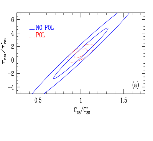
Figure 2: Confidence contours $(68\%\ \&\ 95\%)$ in the $C_{2}^{(S)}-\tau_{ri}$ plane for models in the six parameter space described in the text with (dotted lines) or without (solid lines) polarization information.

We now allow for one more free parameter, the ratio of the tensor to scalar quadrupole anisotropy $T/S$, fixing the tensor spectral index $n_{T}$ using the consistency relation predicted by inflation $T/S=-7n_{T}$ but not assuming a relation between $n_{T}$ and $n_{s}$. The variances for MAP are again summarized in table 1. A comparison with the previous case shows that most variances have increased. Variances for $h$ and $\Omega_{\Lambda}$ are approximately five times larger than before while that for $n_{s}$ has increased by a factor of six and that for $\Omega_{b}h^{2}$ by almost four. On the other hand, the error bar for $\tau_{ri}$ remains unchanged. It is instructive to look again at the contour plots in the $\Omega_{m}-h$ and $\Omega_{b}-h$ planes shown in Figure 1b. The degeneracy on individual parameters is significantly worse because the large angular scale amplitude can now be adjusted freely with the new extra degree of freedom, the tensor to scalar ratio $T/S$. This can therefore compensate any large scale ISW term and so the degeneracy between $h$, $\Omega_{\Lambda}$ and $\Omega_{b}$ cannot be broken as easily. However, a combination of the two parameters is still well constrained as shown in figure 1. The degenerate lines are now given by $\Delta\Omega_{b}/\Omega_{b}+1.66\Delta h/h=0$ and $\Delta\Omega_{m}/\Omega_{m}+3.0\Delta h/h=0$, with relative errors $\Delta(\Omega_{b}h^{1.66})/\Omega_{b}h^{1.66}\approx 4\%$ and $\Delta(\Omega_{m}h^{3})/\Omega_{m}h^{3}\approx 4\%$, almost unchanged from the 6-parameter case. On the other hand for the physically relevant parameters $\Omega_{b}h^{2}$ and $\Omega_{m}h^{2}$ we now have $\Delta(\Omega_{b}h^{2})/\Omega_{b}h^{2}\approx 10\%$ and $\Delta(\Omega_{m}h^{2})/\Omega_{m}h^{2}\approx 25\%$, which is worse than before. This example indicates how the errors on individual parameters can change dramatically as we add more parameters while certain combinations of them remain almost unaffected.

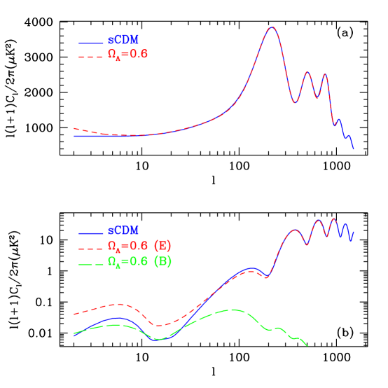
Figure 3: Power spectra of (a) temperature and (b) polarization for two models that will be degenerate for MAP if only temperature information is used. The model with $\Omega_{\Lambda}=0.6$ is the result of the minimization relative to the sCDM for models constrained to have $\Omega_{\Lambda}=0.6$. Polarization helps to break this degeneracy.

The output of a minimization run trying to fit sCDM temperature power spectra with models constrained to have $\Omega_{\Lambda}=0.6$ shows how different parameters can be adjusted in order to keep the power spectrum nearly the same. The minimization program found the model $\hbox{\boldmath{$s$}}_{7}=(610,0.67,0.6,0.03,0.09,1.1,0.68)$ where the last number now corresponds to the $T/S$ ratio, as a model almost indistinguishable from the underlying one. The two models differ by $\Delta\chi^{2}=1.8$ and are shown in figure 3. It is interesting to analyze how different parameters are adjusted to reproduce the underlying model. By adding gravity waves and increasing both the spectral index and the optical depth, the ISW effect from the cosmological constant can be compensated so that it is only noticeable for the first couple of $C_{l}$’s. The relatively high amount of tensors ($T/S\sim 0.7$) lowers the scalar normalization and thus the height of the Doppler peaks, which is compensated by the increase in the spectral index to $n_{s}=1.1$ and the decrease of $\Omega_{m}h^{2}$ from $0.25$ to $0.18$. The latter moves the matter radiation equality closer to recombination increasing the height of the peaks. This is the reason why the degeneracy line is not that of constant $\Omega_{m}h^{2}$ as figure 1 shows. Changes in $\Omega_{m}h^{2}$ change the structure of the peaks and this can be compensated by changing other parameters like the optical depth or the slope of the primordial spectrum. This cannot be achieved across all the spectrum so one can expect that the degeneracy will be lifted as one increases the angular resolution, which is what happens if Planck specifications are used (table 1). Note that the amount of gravity waves introduced to find the best fit does not follow the relation between $n_{T}$ and $n_{s}$ predicted by the simplest inflationary models discussed previously: for $n_{s}=1.1$ no gravity waves are predicted. This explains why the addition of $T/S$ as a free parameter increases the sizes of most error bars compared to the 6-parameter case.

While the two models shown in figure 3 have very similar temperature anisotropy spectra, they make very different astronomical predictions. Figure 4 shows the matter power spectra of the two models. An interesting effect is that the two models are nearly identical on the scale of $k=0.1h$ Mpc^-1, which corresponds to $l\sim k\tau_{0}\sim 600$, the $l$ range where MAP is very sensitive and gravity waves are unimportant. However, the two models differ significantly on the $0.01h$ Mpc^-1 scale and the effective power spectrum shape parameter $\Gamma$ (e.g. Bardeen et al. 1986) is very different for the two models: 0.42 for the matter dominated model and 0.25 for the vacuum dominated model. The current observational situation is still controversial (e.g., Peacock (1996)), but measurements of the spectrum by the Sloan Digital Sky Survey (SDSS) should significantly improve the power spectrum determination. The models also make different predictions for cluster abundances: the matter dominated model has $\sigma_{8}\Omega_{m}^{0.6}=1.2$, while the vacuum dominated model has $\sigma_{8}\Omega_{m}^{0.6}=0.8$. Analysis of cluster X-ray temperature and luminosity functions suggests $\sigma_{8}\Omega_{m}^{0.6}=0.5\pm 0.1$ (Eke et al. (1996)), inconsistent with both of the models in the figure. These kind of measurements can break some of the degeneracies in the CMB data.

Figure 4: Hubble diagram for Type Ia supernovae (a) and CDM linear power spectra (b) for sCDM and the $\Omega_{\Lambda}=0.6$ model described in the text.

Observations of Type Ia supernovae at redshifts $z\sim 0.3-0.6$ is another very promising way of measuring cosmological parameters. This test complements the CMB constraints because the combination of $\Omega_{m}$ and $\Omega_{\Lambda}$ that leaves the luminosity distance to a redshift $z\sim 0.3-0.6$ unchanged differs from the one that leaves the position of the Doppler peaks unchanged. Roughly speaking, the SN observations are sensitive to $q_{0}\simeq\Omega_{m}/2-\Omega_{\Lambda}$, while the CMB observations are sensitive to the luminosity distance which depends on a roughly orthogonal combination, $\Omega_{m}+\Omega_{\Lambda}$. Figure 4a shows the apparent magnitude vs. redshift plot for supernovae in the two models of figure 3. The analysis in Perlmutter et al. (1996) of the first seven supernovae already excludes the $\Omega_{\Lambda}=0.6$ model with a high confidence. However, tt remains to be seen however whether this test will be free of systematics such as evolutionary effects that have plagued other classical cosmological tests based on the luminosity-redshift relation.

Finally, we may also relax the relation between tensor spectral index and its amplitude, thereby testing the consistency relation of inflation. For MAP, we studied two sCDM models, one with $T/S=0.28$ and one with $T/S=0.1$, but with $\tau_{ri}=0.1$, for Planck we only used the latter model. Table 1 summarizes the obtained one sigma limits. A comparison between the $T/S=0.28$ model and previous results for sCDM with seven parameters shows that the addition of $n_{T}$ as a new parameter does not significantly change the expected sensitivities to most parameters. The largest change, as expected, is for the tensor to scalar ratio. We now find $\Delta T/S\sim 0.7$ which means that the consistency relation will only be poorly tested from the temperature measurements. If $T/S=0.1,\tau_{ri}=0.1$ most error bars are smaller than if $T/S=0.28,\tau_{ri}=0.05$ case. The reason for this is that the higher value of the optical depth in the underlying model makes its detection easier and this translates to smaller error bars on the other parameters. The only exception is $n_{T}$, which has significantly higher error if $T/S=0.1$ than if $T/S=0.28$ as expected on the basis of the smaller contribution of tensor modes to the total anisotropies. A comparison between the expected MAP and Planck performances for the $T/S=0.1$ model shows that Planck error bars are significantly smaller. For $h$, $\Omega_{b}h^{2}$ and $\Omega_{\Lambda}$ the improvement is by a factor of $10-20$, while for $T/S$ and $C_{2}^{(S)}$ by a factor of $2-3$. The limits on $\tau_{ri}$ and $n_{T}$ remain nearly unchanged, reflecting the fact that these parameters are mostly constrained on large angular scales which are cosmic variance and not noise/resolution limited. It is for these parameters that polarization information helps significantly, as discussed in the next section.

The accuracy with which certain parameters can be determined depends not only on the number of parameters but also on their “true” value. We tested the sensitivity of the results by repeating the analysis around a cosmological constant model $\hbox{\boldmath{$s$}}_{8}=(922,0.65,0.7,0.06,0.1,1.0,0.1,0.0)$, where the last number corresponds to the tensor spectral index $n_{T}$. Results for MAP specifications are given in table 1. The most dramatic change is for the cosmological constant, which is a factor of ten better constrained in this case. This is because the underlying model has a large ISW effect which increases the anisotropies at small $l$. This cannot be mimicked by adjusting the tensors, optical depth and scalar slope as can be done if the slope of the underlying model is flat, such as for sCDM model in figure 3. Because of the degeneracy between $\Omega_{\Lambda}$ and $h$ , a better constraint on the former will also improve the latter, as shown in table 1. Similarly because a change in $\Omega_{\Lambda}$ affects $T/S$, $\tau_{ri}$ and $n_{s}$ on large scales, the limits on these parameters will also change. On the other hand, errors on $\Omega_{b}h^{2}$, $C_{2}^{(S)}$ and $n_{T}$ do not significantly change. This example clearly shows that the effects of the underlying model can be rather significant for certain parameters, so one has to be careful in quoting the numbers without specifying the “true” parameters of the underlying model as well.

So far we only discussed flat cosmological models. CMBFAST can compute open cosmological models as well, and we will now address the question of how well can curvature be determined using temperature data. We consider models in a six parameter space $\hbox{\boldmath{$s$}}_{6}=(C_{2}^{(S)},h,\Omega,\Omega_{b},\tau_{ri},n_{s})$, with no gravity waves and where $\Omega_{\Lambda}=0$, so that $\Omega=\Omega_{m}$. We will consider as the underlying model $\hbox{\boldmath{$s$}}_{6}=(1122,0.65,0.4,0.06,0.05,1.0)$. Fisher matrix results are displayed in table 1. Within this family of models $\Omega$ can be determined very precisely by both MAP and Planck due to its effect on the position of the Doppler peaks. This conclusion changes drastically if we also allow cosmological constant, in which case $\Omega=\Omega_{m}+\Omega_{\Lambda}$. Both $\Omega$ and $\Omega_{\Lambda}$ change the angular size of the sound horizon at recombination so it is possible to change the two parameters without changing the angular size, hence the two parameters will be nearly degenerate in general. We will discuss this degeneracy in greater detail in the next section, but we can already say that including both parameters in the analysis increases the error bar on the curvature dramatically.

To summarize our results so far, keeping in mind that the precise numbers depend on the underlying model and the number of parameters being extracted, we may reasonably expect that using temperature information only MAP (Planck) will be able to achieve accuracies of $\Delta C_{2}^{(S)}/C_{2}^{(S)}\sim 0.5(0.1)$, $\Delta h\sim 0.1(0.006)$, $\Delta\Omega_{\Lambda}\sim 0.6(0.03)$, $\Delta(\Omega_{b}h^{2})/\Omega_{b}h^{2}\sim 0.1(0.008)$, $\Delta\tau_{ri}\sim 0.1(0.1)$, $\Delta n_{s}\sim 0.07(0.006)$, $\Delta(T/S)\sim 0.7(0.3)$ and $\Delta n_{T}\sim 1(1)$. It is also worth emphasizing that there are combinations of the parameters that are very well constrained, e.g., $\Delta(\Omega_{m}h^{3})/\Omega_{m}h^{3}\sim 0.04$ and $\Delta(C_{2}^{(S)})/C_{2}^{(S)}-2\Delta{\tau_{ri}}\sim 0.05$. For the family of models with curvature but no cosmological constant, MAP (Planck) will be able to achieve $\Delta\Omega\sim 0.007(0.0006)$, determining the curvature of the universe with an impressive accuracy.

These results agree qualitatively, but not quantitatively, with those in Jungman et al. (1996). The discrepancy is most significant for $C_{2}^{(S)}$, $h$ and $\Omega_{\Lambda}$, for which the error bars obtained here are significantly larger. The limit we obtain for $\Omega_{b}h^{2}$ is several times smaller than that in Jungman et al. (1996), while for the rest of the parameters the results agree. The use of different codes for computing model predictions is probably the main cause of discrepancies and emphasizes the need to use high accuracy computational codes when performing this type of analysis.

4 Constraints from temperature and polarization data

In this section, we consider the constraints on cosmological parameters that could be obtained when both temperature and polarization data are used. To generate polarization, two conditions have to be satisfied: photons need to scatter (Thomson scattering has a polarization dependent scattering cross-section) and the angular distribution of the photon temperature must have a non-zero quadrupole moment. Tight coupling between photons and electrons prior to recombination makes the photon temperature distribution nearly isotropic and the generated polarization very small, specially on scales larger than the width of the last scattering surface. For this reason polarization has not been considered previously as being important for the determination of cosmological parameters. However, early reionization increases the polarization amplitude on large angular scales in a way which cannot be mimicked with variations in other parameters (Zaldarriaga (1996)). The reason for this is that after recombination the quadrupole moment starts to grow due to the photon free streaming. If there is an early reionization with sufficient optical depth, then the new scatterings can transform this angular anisotropy into polarization. This effect dominates on the angular scale of the horizon when reionization occurs. It will produce a peak in the polarization power spectrum with an amplitude proportional to the optical depth, $\tau_{ri}$, and a position, $l\sim 2\sqrt{z_{ri}}$, where $z_{ri}$ is the redshift of reionization.

We first consider the six parameter space described in the previous section. Table 2 contains the one sigma errors on the parameters for MAP specifications. Compared to the temperature case, the errors improve particularly on the amplitude, the reionization optical depth and the spectral index $n_{s}$. Figure 2 shows the confidence contours for $C_{2}^{(S)}$ and $\tau_{ri}$ with and without polarization. One can see from this figure how the information in the polarization breaks the degeneracy between the two parameters by reducing the error on $\tau_{ri}$, but does not really improve their non-degenerate combination, which is well determined from the temperature data alone.

We now allow for one more parameter, $T/S$. Again, polarization improves the errors on most of the parameters by a factor of two compared to the no-polarization case, as summarized in table 2. The optical depth and the amplitude are better constrained for the same reason as for the six parameter model discussed above. Without polarization, the extra freedom allowed by the gravity waves made it possible to compensate the changes on large angular scales caused by the ISW, while the amplitude of small scale fluctuations could be adjusted by changing the optical depth and the spectral index. Changing $n_{s}$, also changes the slope on large angular scales compensating the change caused by the ISW. When polarization is included, a change in the optical depth produces a large effect in the spectrum: see the model with $\Omega_{\Lambda}=0.6$ in figure 2, which has $\tau_{ri}=0.1$. The difference in $\chi^{2}$ between the two models in figure 2 becomes 10 instead of 1.8.

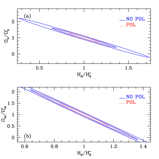
Figure 5: Confidence contours $(68\%\ \&\ 95\%)$ in the (a) $\Omega_{b}-h$ plane and (b) $\Omega_{m}-h$ plane for models in the seven parameter space described in the text with or without using polarization information.

Figure 5 shows how the confidence contours in the $\Omega_{m}-h$ and $\Omega_{b}-h$ planes are improved by including polarization. The $95\%$ confidence contour corresponds roughly to the $68\%$ confidence contour that could be obtained from temperature information alone, while the orientation of the error ellipsoids does not change. As before the well determined combination is constrained from the temperature data alone. The constraints on tensor parameters also improve when polarization is included. Again, this results from the better sensitivity to the ionization history, which is partially degenerate with the tensor contribution, as discussed in the previous section. The $B$ channel to which only gravity waves contribute is not providing additional information in the model with $T/S=0.28$ for MAP noise levels. Even in a model with $T/S=1$ the $B$ channel does not provide additional information in the case of MAP.

With its very sensitive bolometers, Planck has the potential to detect the $B$ channel polarization produced by tensor modes: the $B$ channel provides a signature free of scalar mode contribution (Seljak & Zaldarriaga (1997), Kamionkowski et al. (1997)). However, it is important to realize that even though for a model with $T/S=1$ only $20\%$ of the sensitivity of Planck to tensor modes is coming from the $B$ channel. Planck can detected primordial gravity waves in models with $T/S\sim 0.3$ in the $B$ channel alone. If the bolometer sensitivities are improved so that $w_{P}^{-1}=(0.015\mu K)^{2}$, then Planck can detect gravity waves in the $B$ channel even if $T/S\sim 0.1$. We also analyzed the 8-parameter models presented in table 2. For the models with $T/S=0.28$ and $T/S=0.1$, MAP will not have sufficient sensitivity to test the inflationary consistency relation: $T/S=-7n_{T}$. Planck should have sufficient sensitivity to determine $n_{T}$ with an error of 0.2 if $T/S\sim 0.1$, which would allow a reasonable test of the consistency relation.

Polarization is helping to constrain most of the parameters mainly by better constraining $\tau_{ri}$ and thus removing some of its degeneracies with other parameters. Planck will be able to determine not only the total optical depth through the amplitude of the reionization peak but also the ionization fraction, $x_{e}$, through its position. To investigate this, we assumed that the universe reionized instantaneously at $z_{ri}$ and that $x_{e}$ remains constant but different from 1 for $z<z_{ri}$). The results given in table 2 indicate that $x_{e}$ can be determined with an accuracy of 15%. This together with the optical depth will be an important test of galaxy formation models which at the moment are consistent with wildly different ionization histories and cannot be probed otherwise (Haiman & Loeb (1996), Gnedin & Ostriker (1996)). We also investigated the modified Planck design, where both polarization states in bolometers are measured. An improved polarization noise of $w_{P}^{-1}=(0.015\mu K)^{2}$ for Planck will shrink the error bars presented in table 2 by an additional $6-20\,\%$. Error bars on $\Omega_{\Lambda}$ and $\Omega_{b}h^{2}$ are reduced by $20\%$, those in $h$, $\tau_{ri}$ and $x_{e}$ $10-15\,\%$ and for $T/S$, $n_{T}$ and $n_{s}$ the improvement is approximately $6\%$.

We can examine in more detail how polarization helps to constrain different cosmological parameters by investigating the angular scales in the polarization power spectra that contribute the most information. To do so, we will consider the $T/S=0.1$ model and perform a Fisher matrix analysis that includes all the temperature information, but polarization information only up to maximum $l$. Figures 6 (MAP) and 7 (Planck) show the increase in accuracy as a function of maximum $l$ for various parameters. In the case of Planck, we added the ionization fraction after reionization as another parameter. Most of the increase in information is coming from the low $l$ portion of polarization spectrum, primarily from the peak produced by reionization around $l\sim 10$. The first Doppler peak in the polarization spectra at $l\sim 100$ explains the second increase in information in the MAP case. The better noise properties and resolution of Planck help to reach the higher $l$ polarization Doppler peaks, which add additional information for constraining $h$, $\Omega_{b}h^{2}$ and $\Omega_{\Lambda}$. For Planck, on the other hand, some of the degeneracies will already be lifted in the temperature data alone and so less is gained when polarization data is used to constrain the ionization history.

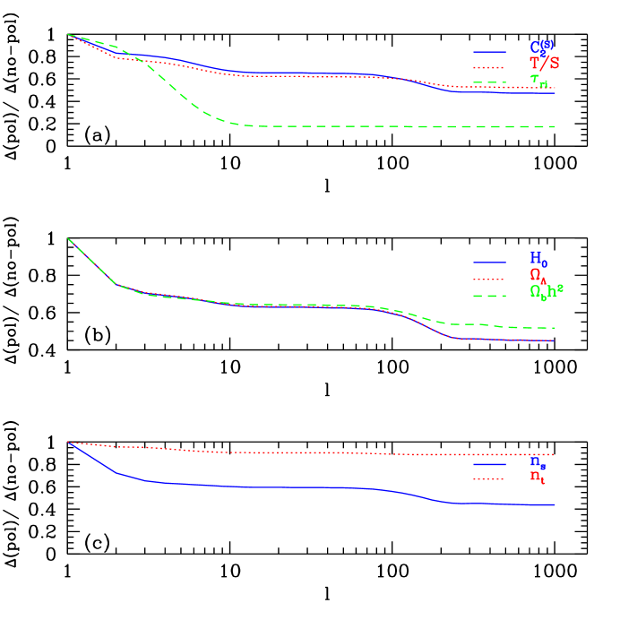
Figure 6: Relative improvement in the parameter estimation as a function of the maximum $l$ up to which polarization information is used for the MAP mission.

Figure 7: Same as figure 6 but for Planck mission parameters.

An interesting question that we can address with the methods developed here is to what extent is one willing to sacrifice the sensitivity in temperature to gain sensitivity in polarization. A specific example is the 140 GHz channel in Planck, where the current proposal is to have four bolometers with no polarization sensitivity and eight bolometers which are polarization sensitive so that they transmit only one polarization state while the other is being thrown away. One can compare the results of the Fisher information matrix analysis for this case with the one where all twelve detectors have only temperature sensitivity, but with better overall noise because no photons are being thrown away. The results in this case for the 8 parameter model with $T/S=0.1$ are 10-20% better than the results given in the fifth column of table 1. These results should be compared to the same case with polarization in table 2. The latter case is clearly better for all the parameters, specially for those that are degenerate with reionization parameters, where the improvement can be quite dramatic. Based on this example it seems clear that it is worth including polarization sensitivity in the bolometer detectors, even at the expense of some sensitivity in the temperature. However, it remains to be seen whether such small levels of polarization can be separated from the foregrounds.

The Fisher matrix results for the six parameter open models are presented in table 2. As expected polarization improved the constraints on $C_{2}^{(S)}$ and $\tau_{ri}$ the most. So far we have explicitly left $\Omega_{\Lambda}$ out of the analysis; as discussed in §3 the positions of the peaks depends on both $\Omega$ and $\Omega_{\Lambda}$ and it is possible to change the two parameters without changing the spectrum. For any given value of $\Omega_{m}$ we may adjust $h$ and $\Omega_{b}$ to keep $\Omega_{b}h^{2}$ and $\Omega_{m}h^{2}$ constant, so that acoustic oscillations will not change. If we then in addition adjust also $\Omega_{\Lambda}$ to match the angular size of the acoustic features, then the power spectra for two models with different underlying parameters remain almost unchanged. As mentioned in previous section the effect of $\Omega_{\Lambda}$ on the positions of the peaks is rather weak around $\Omega_{m}=1$ and the peak positions are mostly sensitive to the curvature $\Omega$. The lines of constant $l_{peak}$, the inverse of the angular size of acoustic horizon, roughly coincide with those of constant $\Omega$ near flat models, making it possible to weigh the universe using the position of the peaks. In the more general case, it is not $\Omega$ that can be determined from the CMB observations. but a particular combination of $\Omega_{m}$ and $\Omega_{\Lambda}$ that leaves $l_{peak}$ unchanged. Figure 8 shows confidence contours in the $\Omega_{m}-\Omega_{\Lambda}$ plane. The contours approximately agree with the constant $l_{peak}$ (dotted) line, which around $\Omega_{m}=1$ coincides with the constant $\Omega$ line (dashed) but not around $\Omega_{m}=0.4$. The squares and triangles correspond to the minima found by the minimization routine when constrained to move in subspaces of constant $\Omega$ and agree with the ellipsoids from the Fisher matrix approach.

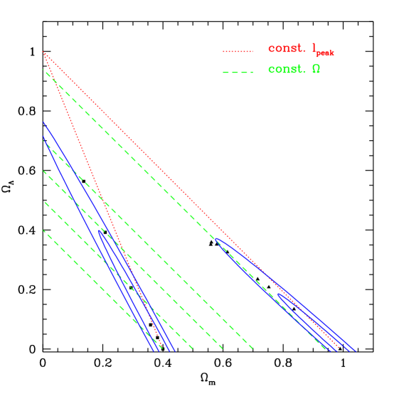
Figure 8: Confidence contours $(68\%\ \&\ 95\%)$ in the $\Omega_{\Lambda}-\Omega_{m}$ plane for open models in the seven parameter space described in the text. The dots show the positions of the $\chi^{2}$ minima found by the minimization routine when constrained to a subspace of constant $\Omega$.

Figure 9 shows the temperature and polarization spectra for the basis model and one found by the minimization routine with $\hbox{\boldmath{$s$}}_{o}=(1495,.87,0.6,0.033,0.051,1.0,0.39)$ where the last number is now $\Omega_{\Lambda}$. This model differs from the basis model by a $\chi^{2}=2$ and so is practically indistinguishable from it. Only on large angular scales do the two models differ somewhat, but cosmic variance prevents an accurate separation between the two. In this case, polarization does not help to break the degeneracy. The agreement on the large angular scales is better for polarization than for temperature because the former does not have a contribution from the ISW effect, which is the only effect that can break this degeneracy. When both $\Omega$ and $\Omega_{\Lambda}$ are included in the analysis the $1\sigma$ error bars for both MAP and Planck increase. The greatest change is for the error bars on the curvature that now becomes $\Delta\Omega=0.1$ for both MAP and Planck. Note that improving the angular resolution does not help to break the degeneracy, which is why MAP and Planck results are similar. If one is willing to allow for both cosmological constant and curvature then there is a genuine degeneracy present in the microwave data and constraints from other cosmological probes will be needed to break this degeneracy.

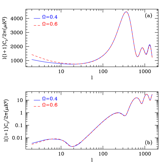
Figure 9: Power spectra for (a) temperature and (b) polarization. The model with $\Omega=0.6,\Omega_{\Lambda}=0.4$ is the output of the minimization code when made to fit the $\Omega=0.4,\Omega_{\Lambda}=0$ model. Temperature and polarization data were used for this fit. the two models differ in $\chi^{2}$ by 2.

5 Shape of the likelihood function, priors and gravitational lensing

As mentioned in §2, the Fisher information matrix approach used so far assumes that the likelihood function is gaussian around the maximum. In previous work (Jungman et al. (1996)), this assumption was tested by calculating the likelihood along several directions in parameter space. This approach could miss potential problems in other directions, particularly when there are degeneracies between parameters. We will further test the gaussian assumption by investigating the shape of the likelihood function varying one parameter at a time but marginalizing over the others. We fix the relevant parameter and let the minimization routine vary all the others in its search for the smallest $\chi^{2}$. We then repeat the procedure for a different value of this parameter, mapping the shape of the likelihood function around the minimum. The minimization routine is exploring parameter space in all but one direction. These results may be compared with the prediction of the Fisher matrix which follow a parabola in the parameter versus log-likelihood plot. This comparison tests the gaussianity of the likelihood function in one direction of parameter space.

The panels in figure 10 show two examples of the results of this procedure. In most cases, the agreement between the Fisher matrix results and those of the minimization code is very good, especially very near the minimum (i.e., $\Delta\chi^{2}\raise 2.9pt\hbox{$\scriptstyle<$}\lower 0.5pt\hbox{$\scriptscriptstyle\sim$}\;2$). As illustrated in the $\Omega_{b}$ panel, there are cases when $\chi^{2}$ increased more rapidly than predicted by the Fisher matrix. This is caused by the requirements that $\tau_{ri}$, $\Omega$, $\Omega_{\Lambda}$ and $\Omega_{b}$ are all positive, which can be enforced easily in the minimization code. Of course, such priors are most relevant if the underlying model is very close to the boundary enforced by the prior and are only important on one side of the parameter space. The importance of this effect therefore depends on the underlying model. If the amount of information in the CMB data on a given parameter is sufficiently high, then the prior will have only a small effect near the maximum of the likelihood function.

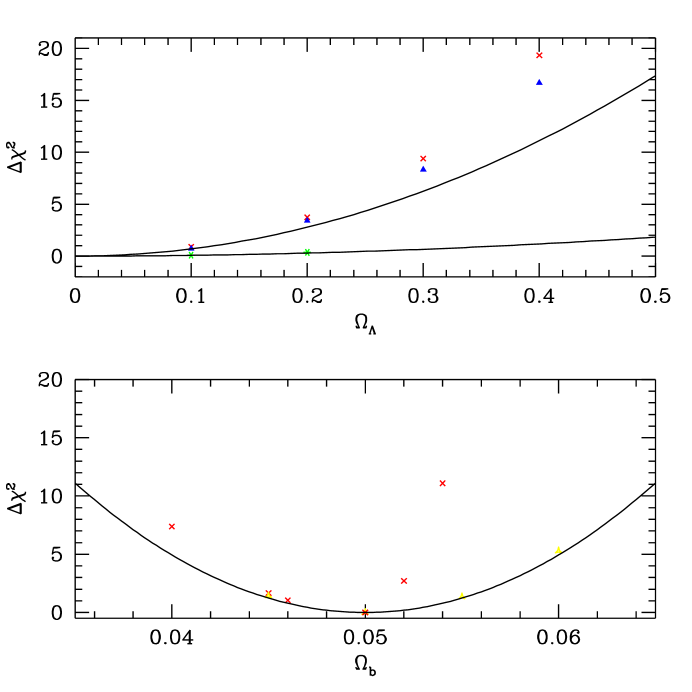
Figure 10: Comparison between the Fisher matrix expansion of the likelihood around the minimum (solid lines) and direct minimization for two different cosmological parameters. In most cases the agreement near the minimum is good. In the upper panel full triangles (crosses) correspond to fits of sCDM within the six parameter family described in the text, including (not including) the effects of gravitational lensing. The lower curve belongs to the $T/S=0.28$ model in the eight parameter space. In the lower panel, the $\Omega_{\Lambda}>0$ prior is reached for sCDM when $\Omega_{b}>0.05$, which is why the minimization results differ from the Fisher matrix results.

We also investigated the effect of gravitational lensing on the parameter reconstruction. As shown in Seljak (1996a), gravitational lensing smears somewhat the acoustic oscillations but leaves the overall shape of the power spectrum unchanged. The amplitude of the effect depends on the power spectrum of density fluctuations. Because the CMBFAST output consists of both CMB and density power spectra one can use them as an input for the calculation of the weak lensing effect following the method in Seljak (1996a). The gravitational lensing effect is treated self-consistently by normalizing the power spectrum for each model to COBE. We find that the addition of gravitational lensing to the calculation does not appreciably change the expected sensitivity to different parameters that will be attained with the future CMB experiments. This conclusion again depends somewhat on the underlying model, but even for sCDM where COBE normalization predicts two times larger small scale normalization than required by the cluster abundance data, the lensing effect is barely noticeable in the error contours for various parameters.

6 Conclusions

In this paper, we have analyzed how accurately cosmological parameters can be extracted from the CMB measurements by two future satellite missions. Our work differs from previous studies on this subject in that we use a more accurate computational code for calculating the theoretical spectra and we include the additional information that is present in the polarization of the microwave background. We also investigate how the results change if we vary the number of parameters to be modeled or the underlying model around which the parameters are estimated. Both of these variations can have a large effect on the claimed accuracies of certain parameters, so the numbers presented here should not be used as firm numbers but more as typical values. Of course, once the underlying model is revealed to us by the observations then these estimates can be made more accurate. The issue of variation of the errors on the number of parameters however remains, and results will always depend to some extent on the prior belief. If, for example, one believes that gravity waves are not generated in inflationary models (e.g., Lyth (1996)) or that they are related to the scalar perturbations through a simple relation (e.g., Turner (1993)), then the MAP errors on most parameters shrink by a factor of 2. Similarly, one may decide that models with both curvature and cosmological constant are not likely, which removes the only inherent degeneracy present in the CMB data.

Using temperature data alone, MAP should be able to make accurate determinations (better than 10%) of the scalar amplitude ($\sigma_{8}$), the baryon/photon ratio ($\Omega_{b}h^{2}$), the matter content ($\Omega_{m}h^{2})$, the power spectrum slope ($n_{s}$) and the angular diameter distance to the surface of last scattering (a combination of $\Omega$ and $\Omega_{\Lambda}$). If we restrict ourselves to models with no gravity wave content, then MAP should also be able to make accurate determinations of $\Omega_{\Lambda}$, the Hubble constant and the optical depth, $\tau_{ri}$. However, in more general models that include gravity wave amplitude and slope as additional parameters, the degeneracies between these parameters are large and they cannot be accurately determined. Several other measurements of the CMB anisotropies from the ground and from balloons are now in progress and very accurate results are likely to be available by the time MAP flies. This additional information will help constrain the models further, specially determinations of the power spectrum at the smaller angular scales. Astronomical data can significantly reduce these degeneracies. The two nearly degenerate models, sCDM and a tilted vacuum dominated model ($\Omega_{\Lambda}=0.6$) shown in figure 2 can be distinguished already by current determinations of $\sigma_{8}\Omega^{0.6}$, or by measurements of the shape parameter $\Gamma$ in the galaxy power spectrum, or by measurements of the distance-magnitude relationship with SN Ia’s.

MAP’s measurements of polarization will significantly enhance its scientific return. These measurements will accurately determine the optical depth between the present and the surface of last scatter. This will not only probe star formation during the “dark ages” ($5<z<1300$), but will also enable accurate determination of the Hubble constant and help place interesting constraints on $\Omega_{\Lambda}$ in models with tensor slope and amplitude as free parameters.

Planck’s higher sensitivity and smaller angular resolution will enable further improvements in the parameter determination. Particularly noteworthy is its ability to constrain $\Omega_{\Lambda}$ to better than 5% and the Hubble constant to better than 1% even in the most general model considered here. The proposed addition of polarization sensitive bolometer channels to Planck significantly enhances its science return. Planck should be able to measure the ionization history of the early universe, thus studying primordial star formation. Sensitive polarization measurements should enable Planck to determine the amplitude and slope of the gravity wave spectrum. This is particularly exciting as it directly tests the predicted tensor/scalar relations in the inflationary theory and is a probe of Planck scale physics. The primordial gravity wave contribution can at present only be measured through the CMB observations. One may therefore ask how well Planck can determine $T/S$ assuming that other cosmological parameters are perfectly known by combining CMB and other astronomical data. The answer sensitively depends on reionization optical depth. Without reionization, $T/S\sim 0.1$ can be detected, while with $\tau_{ri}=0.1$ this number drops down to $T/S\sim 0.02$. The equivalent number without polarization information is $0.2$, regardless of optical depth. Improvements in sensitivity will further improve these numbers, particularly in the $B$ polarization channel which is not cosmic variance limited in the sense that tensors cannot be confused with scalars. A detection of a $B$ component would mean a model independent detection of a stochastic background of gravitational waves or vector modes (Seljak & Zaldarriaga 1997).

The most exciting science return from polarization measurements come from measurements at large angular scales (see figures 6 & 7). These measurements can only be made from satellites as systematic effects will swamp balloons and ground based experiments on these scales. The low $l$ measurements enable determinations of the optical depth and the ionization history of the universe and may lead to the detection of gravity waves from the early universe. Both foregrounds and systematic effects may swamp the weak polarization signal, even in space missions, thus it is important that the satellite experiment teams adopt scan strategies and frequency coverages that can minimize systematics and foregrounds at large angles.

We explored the question of how priors such as positivity of certain parameters or constraints from other cosmological probes help reduce the uncertainties from the CMB data alone. For this purpose, we compared the predictions from the Fisher information matrix with those of the brute-force minimization which allows the easy incorporation of inequality priors. As expected, we find that positivity changes the error estimates only on the parameters that are not well constrained by the CMB data. On the other hand, using some additional constraints such as the limits on the Hubble constant, age of the universe, dark matter power spectrum or $q_{0}$ measurements from type Ia supernovae can significantly reduce the error estimates because the degeneracies present in these cosmological tests are typically different from those present in the CMB data. The minimization approach also allows testing the assumption that the log-likelihood is well described by a quadratic around the minimum, which is implicit in the Fisher matrix approach. We find that this is a good approximation close to the minimum, with no nearby secondary minima that could be confused with the global one. Finally, we also tested the effect of gravitational lensing on the reconstruction of parameters and found that its effect on the shape of the likelihood function can be neglected.

In summary, future CMB data will provide us with an unprecedented amount of information in the form of temperature and polarization power spectra. Provided that the true cosmological model belongs to the class of models studied here these data will enable us to constrain several combinations of cosmological parameters with an exquisite accuracy. While some degeneracies between the cosmological parameters do exist, and in principle do not allow some of them to be accurately determined individually, these can be removed by including other cosmological constraints. Some of these degeneracies belong to contrived cosmological models, which may not survive when other considerations are included. The microwave background is at present our best hope for an accurate determination of classical cosmological parameters.

$Param.$	${\rm sCDM}^{+}$	${\rm sCDM}^{+}$	${T\over S}=0.28^{+}$	${T\over S}=0.1^{+}$	${T\over S}=0.1^{\times}$	$\Omega_{\Lambda}=0.7^{+}$	Open+	Open×
$\Delta\ln C_{2}^{(S)}$	$2.1\,10^{-1}$	$4.2\,10^{-1}$	$4.8\,10^{-1}$	$4.7\,10^{-1}$	$7.4\,10^{-2}$	$4.1\,10^{-1}$	$1.2\,10^{-1}$	$4.7\,10^{-2}$
$\Delta h$	$1.7\,10^{-2}$	$9.2\,10^{-2}$	$1.1\,10^{-1}$	$1.0\,10^{-1}$	$5.1\,10^{-3}$	$4.1\,10^{-2}$	$2.0\,10^{-2}$	$1.1\,10^{-3}$
$\Delta\Omega_{\Lambda}$	$9.8\,10^{-2}$	$5.3\,10^{-1}$	$6.1\,10^{-1}$	$5.8\,10^{-1}$	$2.9\,10^{-2}$	$5.0\,10^{-2}$	-	-
$\Delta\Omega_{b}h^{2}$	$3.0\,10^{-4}$	$1.0\,10^{-3}$	$9.8\,10^{-4}$	$1.2\,10^{-3}$	$1.2\,10^{-4}$	$9.7\,10^{-4}$	$1.1\,10^{-3}$	$1.3\,10^{-4}$
$\Delta\tau_{ri}$	$1.2\,10^{-1}$	$1.3\,10^{-1}$	$1.4\,10^{-1}$	$1.1\,10^{-1}$	$8.2\,10^{-2}$	$1.9\,10^{-1}$	$7.2\,10^{-2}$	$3.3\,10^{-2}$
$\Delta n_{s}$	$9.8\,10^{-3}$	$5.9\,10^{-2}$	$6.7\,10^{-2}$	$6.4\,10^{-2}$	$5.9\,10^{-3}$	$2.9\,10^{-2}$	$2.4\,10^{-2}$	$3.3\,10^{-3}$
$\Delta{T\over S}$	-	$3.9\,10^{-1}$	$6.8\,10^{-1}$	$5.3\,10^{-1}$	$2.5\,10^{-1}$	$3.2\,10^{-1}$	-	-
$\Delta n_{T}$	-	-	$3.9\,10^{-1}$	$9.1\,10^{-1}$	$9.4\,10^{-1}$	$9.9\,10^{-1}$	-	-
$\Delta\Omega$	-	-	-	-	-	-	$6.6\,10^{-3}$	$5.2\,10^{-4}$

Table 1. Fisher matrix one-sigma error bars for different cosmological parameters when only temperature is included. Table 3 gives the cosmological parameters for each of the models. Columns with $+$ correspond to MAP and those with $\times$ to Planck.

$Param.$	${\rm sCDM}^{+}$	${\rm sCDM}^{+}$	${T\over S}=0.28^{+}$	${T\over S}=0.1^{+}$	${T\over S}=0.1^{\times}$	$\Omega_{\Lambda}=0.7^{+}$	Open+	Open×
$\Delta\ln C_{2}^{(S)}$	$4.8\,10^{-2}$	$2.4\,10^{-1}$	$2.8\,10^{-1}$	$2.4\,10^{-1}$	$1.0\,10^{-2}$	$8.3\,10^{-2}$	$6.5\,10^{-2}$	$1.2\,10^{-2}$
$\Delta h$	$1.6\,10^{-2}$	$5.1\,10^{-2}$	$5.8\,10^{-2}$	$5.0\,10^{-2}$	$3.0\,10^{-3}$	$3.8\,10^{-2}$	$1.9\,10^{-2}$	$1.0\,10^{-3}$
$\Delta\Omega_{\Lambda}$	$9.3\,10^{-2}$	$2.9\,10^{-1}$	$3.3\,10^{-1}$	$2.9\,10^{-1}$	$1.7\,10^{-2}$	$4.6\,10^{-2}$	-	-
$\Delta\Omega_{b}h^{2}$	$2.8\,10^{-4}$	$6.1\,10^{-4}$	$7.1\,10^{-4}$	$6.2\,10^{-4}\$	$5.7\,10^{-5}\$	$8.9\,10^{-4}$	$9.5\,10^{-4}$	$1.1\,10^{-4}$
$\Delta\tau_{ri}$	$2.1\,10^{-2}$	$2.1\,10^{-2}$	$2.0\,10^{-2}$	$2.0\,10^{-2}$	$5.5\,10^{-3}$	$2.0\,10^{-2}$	$3.2\,10^{-2}$	$3.5\,10^{-3}$
$\Delta n_{s}$	$4.8\,10^{-3}$	$3.1\,10^{-2}$	$3.5\,10^{-1}$	$3.0\,10^{-2}$	$3.0\,10^{-3}$	$2.6\,10^{-2}$	$1.7\,10^{-2}$	$2.6\,10^{-3}$
$\Delta{T\over S}$	-	$2.2\,10^{-1}$	$4.3\,10^{-1}$	$3.0\,10^{-1}$	$4.5\,10^{-2}$	$2.1\,10^{-1}$	-	-
$\Delta n_{T}$	-	-	$3.9\,10^{-1}$	$8.1\,10^{-1}$	$1.7\,10^{-1}$	$7.8\,10^{-1}$	-	-
$\Delta x_{e}$	-	-	-	-	$1.4\,10^{-1}$	-	-	-
$\Delta\Omega$	-	-	-	-	-	-	$6.1\,10^{-3}$	$4.1\,10^{-4}$

Table 2. Fisher matrix one-sigma error bars for different cosmological parameters when both temperature and polarization is included. Table 3 gives the cosmological parameters for each of the models. Columns with $+$ correspond to MAP and those with $\times$ to Planck.

$Param.$	${\rm sCDM}$	${T\over S}=0.28$	${T\over S}=0.1$	$\Omega_{\Lambda}=0.7$	Open
$h$	$0.5$	$0.5$	$0.5$	$.65$	$.65$
$\Omega_{\Lambda}$	$0.0$	$0.0$	$0.0$	$0.7$	$0.0$
$\Omega_{b}$	$0.05$	$0.05$	$0.05$	$0.06$	$0.06$
$\tau_{ri}$	$0.05$	$0.05$	$0.1$	$0.1$	$0.05$
$n_{s}$	$1.0$	$0.96$	$0.99$	$1.0$	$1.0$
${T\over S}$	$0.0$	$0.28$	$0.1$	$0.0$	$0.0$
$n_{T}$	-	$0.04$	$0.01$	-	-
$\Omega$	$1.0$	$1.0$	$1.0$	$1.0$	$0.4$

Table 3. Cosmological parameters for the models we studied. All models were normalized to COBE.

References

- Bardeen et al. (1986)
- (2) ardeen, J. M., Bond, J. R., Kaiser, N., & Szalay, A. S. 1986, ApJ, 304, 15
- Bennett et al. (1996) Bennett, C. L. et al. 1996, Astrophys. J. 464, L1
- Bond (1996)
- (5) ond, J. R. 1996, in Cosmology and Large Scale Structure, ed R. Schaeffer et. al. (Elsevier Science: Netherlands)
- Bond and Efstathiou (1987) Bond, J. R. & Efstathiou, G. 1987, MNRAS, 226, 655
- Bond et al. (1994) Bond, J. R. et. al. 1994, Phys. Rev. Lett., 72, 13
- Bond et al. (1997) Bond, J. R. et. al. 1997, Report no. astro-ph/9702100 (MNRAS in press)
- Chandrasekhar (1960) Chandrasekhar, S. 1960, in Radiative Transfer (Dover: New York)
- Crittenden et al. (1993) Crittenden R., Davis, R. L. & Steinhardt, P. J. 1993, ApJ, 417, L13
- Efstathiou (1996) Efstathiou, G. 1996, private communication
- Eke et al. (1996) Eke, V. R., Cole, S. & Frenk, C. S. 1996, Report no. astro-ph/9601088 (unpublished)
- Gay (1990) Gay, D. M. 1990, Computing Science Report No. 153, AT&T Bell Laboratories
- Gelfand et al. (1963) Gelfand, I. M., Minlos, R. A. & Shapiro, Z. Ya. 1963, Representations of the rotation and Lorentz groups and their applications (Pergamon: Oxford)
- Gnedin & Ostriker (1996) Gnedin, N. & Ostriker, J. P. 1996, Report no. astro-ph/9612127 (unpublished)
- Goldberg et al. (1967) Goldberg, J. N., et al. 1967, J. Math. Phys. 8, 2155
- Haiman & Loeb (1996) Haiman, Z. & Loeb, A. 1996, Report no. astro-ph/9608130 (unpublished)
- Hu et al. (1995)
- (19) u, W., Scott, D., Sugiyama, N. & White, M. 1995, Phys.Rev. D 52, 5498
- Hu & Sugiyama (1995) Hu, W. & Sugiyama, N. 1995, Astrophys. J., 436, 456
- Jungman et al. (1996) Jungman, G., Kamionkowski, M., Kosowsky, A. & Spergel, D. N. 1996, Phys. Rev. Lett. 76, 1007; 1996, Phys. Rev. D 54 1332
- Kaiser (1983) Kaiser, N. 1983, MNRAS, 202, 1169
- Kamionkowski et al. (1997) Kamionkowski, M., Kosowsky, A. & Stebbins, A. 1997, Phys. Rev. Lett., 78, 2058
- Knox (1995) Knox L., 1995, Phys.Rev. D 52, 4307
- Kofman & Starobinsky (1985)
- (26) ofman, L. & Starobinsky, A. 1985, Sov. Astron. Lett., 11, 271
- Lyth (1996) Lyth, D. H. 1997, Phys. Rev. Lett., 78, 1861
- Ma & Bertschinger (1995) Ma, C. P. & Bertschinger, E. 1995, Astrophys. J. 455, 7
- Newman & Penrose (1966) Newman, E. & Penrose, R. 1966, J. Math. Phys. 7, 863
- Peacock (1996) Peacock, J. A. 1996, astro-ph/9608151 (unpublished)
- Perlmutter et al. (1996) Perlmutter, S., et al. 1996, Report no. astro-ph/9608192 (unpublished)
- Polnarev (1985) Polnarev, A. G. 1985, Sov. Astron. 29, 607
- Seljak (1994) Seljak, U. 1994, Astrophy. J., 435, L87
- (34) Seljak, U. 1996a, Astrophys. J., 463, 1
- (35) Seljak, U. 1996b, ApJ, in press; Report no. astro-ph/9608131
- Seljak & Zaldarriaga (1996) Seljak, U. & Zaldarriaga, M. 1996, Astrophys. J. 469, 7
- Seljak & Zaldarriaga (1997) Seljak, U. & Zaldarriaga, M. 1997, Phys. Rev. Lett., 78, 2054
- Smoot et al. (1992) Smoot, G. F., et al. 1992, ApJ, 396, L1
- Spergel (1994) Spergel, D.N., Warner Prize Lecture, 1994, BAAS, 185.7301
- Tegmark & Efstathiou (1996) Tegmark, M. & Efstathiou G., 1996, MNRAS, 281, 1297
- Tegmark et al. (1996) Tegmark, M., Taylor, A. N. & Heavens, A. F. 1997, ApJ, 480, 22
- Turner (1993) Turner, M. S. 1993, Phys. Rev. D, 48, 4613
- Zaldarriaga (1996) Zaldarriaga, M. 1996, Phys. Rev. D, 55, 1822
- Zaldarriaga and Seljak (1997) Zaldarriaga, M. & Seljak, U. 1997, Phys. Rev. D, 55, 1830