Voids in the Large-Scale Structure

Abstract

Voids are the most prominent feature of the large-scale structure of the universe. Still, they have been generally ignored in quantitative analysis of it, essentially due to the lack of an objective tool to identify the voids and to quantify them. To overcome this, we present here the void finder algorithm, a novel tool for objectively quantifying voids in the galaxy distribution. The algorithm first classifies galaxies as either wall galaxies or field galaxies. Then, it identifies voids in the wall galaxy distribution. Voids are defined as continuous volumes that do not contain any wall galaxies. The voids must be thicker than an adjustable limit, which is refined in successive iterations. In this way we identify the same regions that would be recognized as voids by the eye. Small breaches in the walls are ignored, avoiding artificial connections between neighboring voids.

We test the algorithm using Voronoi tessellations. By appropriate scaling of the parameters with the selection-function we apply it to two redshift surveys, the dense SSRS2 and the full-sky IRAS 1.2 Jy. Both surveys show similar properties: $\sim 50\%$ of the volume is filled by the voids. The voids have a scale of at least 40$\>h^{-1}\>\mbox{Mpc}$, and an average under-density of $-0.9$. Faint galaxies do not fill the voids, but they do populate them more than bright ones. These results suggest that both optically and IRAS selected galaxies delineate the same large-scale structure. Comparison with the recovered mass distribution further suggests that the observed voids in the galaxy distribution correspond well to under-dense regions in the mass distribution. This confirms the gravitational origin of the voids.

1 Introduction

Perhaps one of the most intriguing findings of dense and complete nearby redshift surveys has been the discovery of large voids on scales of $\sim 50\mbox{$\>h^{-1}\>\mbox{Mpc}$}$, and that such large voids appear to be a common feature of the galaxy distribution. Early redshift surveys like the Coma/A1367 survey (Gregory & Thompson 1978) and the Hercules/A2199 survey (Chincarini et al. 1981) gave the first indications for the existence of voids, each revealing a void with a diameter of $\sim 20\mbox{$\>h^{-1}\>\mbox{Mpc}$}$. Surprising as these findings may have been, it was not before the discovery of the Boötes void (Kirshner et al. 1981) that the voids caught the attention of the astrophysical community (for a review, see Rood 1988).

The unexpectedly large void found in the Boötes constellation, confirmed to have a diameter of $\sim 60\mbox{$\>h^{-1}\>\mbox{Mpc}$}$ (Kirshner et al. 1987), brought up the question whether the empty regions we observe are a regular feature of the distribution of galaxies, or rather rare exceptions. Wide-angle yet dense surveys, initially two-dimensional and more recently three-dimensional, probing relatively large volumes of the nearby universe, established that the voids are indeed a common feature of the large-scale structure (LSS) of the universe. The publication of the first slice from the CfA redshift survey (de Lapparent, Geller & Huchra 1986) introduced the picture of a universe where the galaxies are located on the surfaces of bubble-like structures, with diameters in the range 25–50$\>h^{-1}\>\mbox{Mpc}$. The extensions of the CfA survey (Geller & Huchra 1989), complemented in the south hemisphere by the SSRS and its extension, the SSRS2 (da Costa et al. 1988; 1994) have shown that not only large voids exist, but more importantly—that they occur frequently (at least judging by eye), suggesting a compact network of voids filling the entire volume.

It has been recognized early on that inhomogeneities on such scales could impose strong constraints on theoretical models for the formation of LSS. However, the voids have been largely ignored and their incorporation into our theories of LSS has been relatively recent (Blumenthal et al. 1992; Dubinski et al. 1993; Piran et al. 1993). The major obstacle confronting the incorporation of voids into models of LSS has been the difficulty of developing proper tools to identify and to quantify them in an objective manner. As such, the description of a void-filled universe with a characteristic scale of 25–50$\>h^{-1}\>\mbox{Mpc}$ relied solely on the visual impression of redshift maps. In order to make a more quantitative analysis we have developed an algorithm (void finder) for the automatic detection of voids in three-dimensional surveys. Unlike other statistical measures (e.g., the VPF), our target is to identify the individual voids, in as much the same way as voids are identified by eye. The main features of the algorithm are:

1. It is based on the point-distribution of galaxies, without introducing any smoothing scale which destroys the sharpness of the observed features.

2. It allows for the existence of some galaxies within the voids, recognizing that voids need not be completely empty.

3. It attempts to avoid the artificial connection between neighboring voids through small breaches in the walls, realizing that walls in the galaxy distribution need not be homogeneous as small-scale clustering will always be present.

After a review of earlier works (§2), we present a detailed description of our algorithm (§3). We use Voronoi tessellations as a test bed for the algorithm in §4. We then apply the algorithm to the SSRS2 redshift survey (§5). Finally (§6), we compare the voids found in SSRS2 and in IRAS 1.2 Jy, and discuss the results.

2 Earlier Works

The various methods for describing the void content of the LSS of the universe can be divided into two categories: statistical measures, and algorithms for identifying individual voids within a sample.

The major statistical tool used for describing the voids is the Void Probability Function (VPF). It measures the probability $P_{0}(V)$ that a randomly positioned sphere of volume $V$ contains no galaxies (White 1979). For a completely uncorrelated (Poissonian) distribution, it is:

$$P_{0}(V)=\exp(-nV)$$ (1)

where $n$ is the number-density of galaxies, so that any departure from this quantity represents the signature for the presence of clustering. The major drawback of the VPF is that it is very sensitive to the details of the galaxy distribution. For instance, adding a few galaxies in the under-dense regions may greatly modify the VPF. A less sensitive variant of the VPF is the Under-dense Probability Function (UPF), defined as the probability $P_{\delta\rho/\rho}(V)$ that a randomly positioned sphere of volume $V$ has a $\delta\rho/\rho$ under-density (Little & Weinberg 1994).

The first zero-crossing of the two-point correlation function $\xi(r)$ was used by Goldwirth et al. (1995) for determining the maximum diameters of voids in case of spherical voids. The two-point correlation function is defined as the probability in excess of Poisson distribution of finding a galaxy in a volume $\delta V$ at a distance $r$ away from a randomly chosen galaxy:

$$\delta P=n\,\delta V\,[1+\xi(r)]$$ (2)

where $n$ is the mean galaxy number-density. For a cellular like distribution the first-zero crossing is a direct measure of the characteristic size of the cells. Using Voronoi tessellations, they show that despite the large uncertainty in the determination of $\xi(r)$ on large scales ($>20\mbox{$\>h^{-1}\>\mbox{Mpc}$}$), the zero-crossing statistic may be a useful tool in determining the scale of typical voids—if the galaxy distribution is void-filled, and if there is a characteristic scale for the void distribution. Both these questions are addressed here. Examining the SSRS2 sample, it was found that $R_{\rm zero}\approx 38\mbox{$\>h^{-1}\>\mbox{Mpc}$}$.

Previous works have used various definitions for voids, and applied different algorithms to identify them. Perhaps the first work identifying voids in a quantitative manner is that of Pellegrini et al. (1989), who examined ensembles of contiguous cells with densities below a given threshold. They use a cubic lattice, and define a local density for each cell in the lattice. This local density is based on the analysis of the smoothed density field, constructed from the original discrete galaxy distribution. Groups of cells with densities below a specific limit constitute the voids. The algorithm considers two cells as contiguous if they are in contact either through their faces, edges or vertices. This technique was applied to the original SSRS, identifying 4 to 8 voids, depending on the density threshold. Unfortunately, there is only partial overlap between the SSRS and the SSRS2. Thus, an overall comparison between the results is impossible (where possible, corresponding voids are indicated in Table 1). The major shortcomings of this algorithm are its use of a smoothed density field, and the lack of sense of the shape of the void it recognizes, allowing for practically any void shape.

Kauffmann & Fairall (1991, hereafter KF91) designed a more elaborate algorithm. They too used (empty) cubes, to which adjacent faces are attached. However, in order to avoid long finger-like extensions leading from one void into other voids, they impose a constraint on the adjacent faces, that each face must have an area of no less than two-thirds that of the surface on to which it was to be added. This scheme is restrictive, as it is tailored for finding only ellipsoidal-shaped voids. The algorithm was applied to the Southern Redshifts Catalog (SRC) and to an all-sky catalog, finding a peak in the spectrum of void diameters between 8 and 11$\>h^{-1}\>\mbox{Mpc}$.

Only $\sim 10$ (out of $>100$) of the voids found in KF91 are located within the boundaries of the SSRS2. About half of the KF91 voids have an equivalent diameter $d<20\mbox{$\>h^{-1}\>\mbox{Mpc}$}$, which we believe to be statistically insignificant (see §3.3). Other KF91 voids are much smaller than their counterparts identified by the void finder: the Sculptor void (void 5 here) is 40% larger in our analysis, and other voids we find are up to three times larger than the corresponding KF91 voids. The limited algorithm and the different statistical analysis have resulted in a small void diameter, not describing the true nature of the void distribution.

A more recent work applying another void search algorithm, is that of Lindner et al. (1995). In this work single spheres, that are devoid of a certain type of galaxies (depending on the morphological type and luminosity), are used. The algorithm is applied to an area north of the super-galactic (SG) plane, showing that voids defined by bright elliptical galaxies have a mean diameter of up to 40$\>h^{-1}\>\mbox{Mpc}$, in agreement with the void finder results. When considering fainter galaxies, the voids are smaller, with the faintest galaxies studied defining 8$\>h^{-1}\>\mbox{Mpc}$ voids, suggesting that faint galaxies delineate smaller voids within larger ones, which are defined by the bright galaxies.

3 The Void Finder Algorithm

The void finder algorithm was designed with the following conceptual picture in mind: The main features of the LSS of the universe are voids surrounded by walls. The walls are generally thin, two-dimensional structures characterized by a high density of galaxies. They constitute boundaries between under-dense regions, generally ellipsoidal in shape—the voids. Although coherent over large scales, the walls—being subject to small-scale clustering—are not homogeneous and contain small breaches which we wish to ignore. Galaxies within walls are hereafter labeled wall galaxies, while the non-wall galaxies are named field galaxies. The voids are not totally empty: there are a few galaxies in them, which we call void galaxies. The void galaxies are a sub-population of the field galaxies, indicating which of the field galaxies are in the voids. Wall galaxies, on the other hand, cannot—by definition—be in a void.

We define a void as a continuous volume that does not contain any wall galaxies and is nowhere thinner than a given diameter. In other words, one can freely move a sphere with the minimal diameter all through the void. This definition does not pre-determine the shape of the void: it can be a sphere, an ellipsoid, or have a more complex shape, including a non-convex one. The definition is targeted at identifying the same regions that would be recognized as voids, when interpreting a point distribution by eye. As the voids are defined based on the point distribution of galaxies, we do not need to introduce any smoothing scale. This is especially important since one of our goals is to measure the volumes of the voids. As the regions containing most of the galaxies—walls or filaments—are thinner than $\sim 10\mbox{$\>h^{-1}\>\mbox{Mpc}$}$, even relatively small smoothing scales will spread the dense regions into the under-dense ones, artificially diminishing the voids.

Our voids may contain galaxies. A stiffer requirement, such that voids should be completely empty, is too restrictive as a single galaxy located in the middle of what we would like to recognize as a void might prevent its identification. However, for this definition to be practical we must be able to identify the field galaxies before we can start locating the voids.

The algorithm is divided into two steps. First the wall builder identifies the wall galaxies and the field galaxies. Then the void finder locates the voids in the wall galaxy distribution. All together, our method incorporates three parameters, which we define below. Two of these parameters ($n$ and $\beta$) are used to determine the field galaxies; the third parameter ($\xi$) is used during the void search. Specific values for these parameters were chosen after a trial-and-error procedure with various simulations (§4), to give results that resemble as much as possible eye-estimates of the voids.

3.1 The Wall Builder Phase

We define a wall galaxy as a galaxy that has at least $n$ other wall galaxies within a sphere of radius $\ell$ around it. The radius $\ell$ is hereafter referred to as the wall separation distance. A galaxy that does not satisfy this definition is classified as a field galaxy. This is a recursive definition which we apply successively until all the galaxies are classified. The minimal value that enables filtering of long thin chains of galaxies is $n=3$. The choice $n=2$ allows thin chains extending between dense structures. With $n=3$ the minimal structure that can be recognized as a wall is a pyramid-like 4-galaxy cluster, with all distances between these galaxies smaller than $\ell$. The wall separation distance $\ell$ is chosen in the following manner: Let the distance to the $n$’th closest neighbor of a galaxy be $l_{n}$. For a given sample this quantity has an average value $\bar{l}_{n}$ and a standard deviation $\sigma_{n}$. The radius $\ell$ is defined as:

$$\ell\equiv\bar{l}_{n}+\beta\sigma_{n}$$ (3)

We have chosen here $n=3$ and $\beta=1.5$.

Fig. 1 demonstrates how the wall builder works for $n=3$. Notice how the galaxy string is filtered, while the dense structures (upper and lower parts of each panel) are identified and maintained. Additional examples of the wall builder, using Voronoi tessellations, are presented in §4. As a side-bonus of this procedure, originally dedicated to filtering the field galaxies, we obtain a visual identification of the walls. This is done by drawing all the links between wall galaxies satisfying:

$${\mathrm{dist}}(\vec{x}_{i},\vec{x}_{j})<\ell$$ (4)

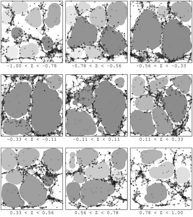
Figure 6: The void finder reconstruction corresponding to Fig. 5: The voids are indicated using various gray shades, where the depicted voids correspond to the intersection of the central plane of each slab with the three-dimensional voids. Also shown are the walls (dark lines—connections between nearby galaxies which satisfy eq. [4]) and the galaxy breakdown (wall galaxies: ‘$\circ$’ or ‘•’; field galaxies, outside the voids: ‘$\oplus$’; void galaxies: ‘$\odot$’). Non-void galaxies that look as if they are in the voids are actually not—they only seem so, due to projection effects. Voids in the first and last panels are smaller due to boundary effects.

These connections are not used in the next step of void analysis, but provide us with another visual tool to examine our results (e.g., see Fig. 6).

3.2 The Void Finder Phase

The void finder searches for spheres that are devoid of any wall galaxies. These spheres are used as building blocks for the voids. A single void is composed of as many (or as few) superimposing spheres as required for covering all of its volume. The algorithm is iterative, initially identifying voids containing relatively large empty spheres, than proceeding to voids containing smaller spheres. The process can be stopped at any desired void resolution, defined as the diameter $d$ of the minimal sphere used as a void building-block. For practical reasons the actual process of improving the resolution is done in discrete iterations. We denote by $d_{\tt i}$ the void resolution used during the $i$’th iteration. Thus, a void containing a sphere of diameter larger than $d_{\tt i}$ would have been identified during the $i$’th iteration, if not earlier. On the other hand, if the largest sphere in a void is smaller than $d_{\tt i}$, that void would not have been identified (yet).

The motivation for using this gradual process of refining the resolution is the problem of keeping apart neighboring voids. If voids were always well-separated by easily recognized homogeneous over-dense regions, there would not be any reason to go through this complicated process. One could simply start from an initial sphere, located somewhere in the void, and work his way from that sphere until he is stopped by a wall. Doing this in all directions and from all spheres would surely be enough to encompass the whole void. However, the situation is more complicated. The walls are not homogeneous, often missing a few bricks now and again. Our eyes are capable of ignoring these breaches in the walls, still identifying the voids as individual objects. For an algorithm aimed at objectively identifying the voids, this is a major problem: how to keep apart neighboring voids, when the boundary is not well marked? A simple application of the above process would result in one all-connected void, since distinct voids would merge with finger-shaped connections passing through the gaps in the walls, in this way connecting those that should have been kept separate.

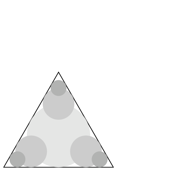
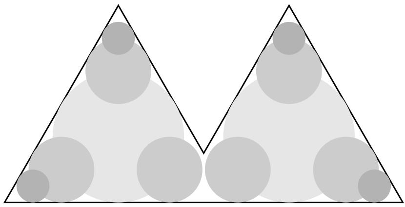
Figure 2: Void coverage using spheres: Larger spheres (light gray) are identified first, and smaller ones (darker gray shades) are identified later. Left: A triangular void. Seven spheres cover the void, the radius of the smallest spheres is a quarter of that of the largest one. Right: Two triangles partially overlapping, as if there is a breach in the wall separating the voids. The gap is larger than the smallest sphere used to cover each void. However, we still can separate the two voids.

The size of the spheres per se is not a good criterion for differentiating between a sphere which is a part of the void proper, and a sphere that is passing through a wall making a false connection. To illustrate this we will use the somewhat artificial example of triangular voids (see Fig. 2, left triangle). To cover a large fraction of this void, one sphere is perhaps sufficient. But to reproduce faithfully the original void, several spheres with various diameters are required—some of the additional spheres being quite small, compared to the initial one. Now, imagine a situation where the two voids are not ideally separated—the two triangles somewhat overlap (Fig. 2, right-hand side). We find that spheres of the same size cover the volume of the voids near the remote edges, but also might connect the two voids to one.

By using a gradually refined void resolution, we overcome this problem in most situations. At the risk of being tautological, we will note that the difference between the void proper and a false connection is that the connections are characterized by them being thinner than the rest of the void and leading into another void. These two properties are critical for our purpose. The first property allows for the initial identification of the center of the void, before finding out about the connections. Using a relatively crude resolution, we will first find the larger spheres that actually make up the void. Now, when the resolution becomes sufficiently small to allow spheres to cross the walls, we will discover that the other side of the wall is already occupied by another void (identified earlier).

Hence, the spheres for covering a void are picked up in two stages: the identification stage, followed by consecutive enhancements. We will now describe these stages in detail.

The identification stage identifies the central parts of the void. Usually, these spheres cover only about half of the actual volume. We focus (at this stage) on identifying a certain void as a separate entity, rather than trying to capture all of its volume. The central parts of a void are covered using spheres with diameters in the range $\xi\mbox{$d_{\rm max}$}<d\leq\mbox{$d_{\rm max}$}$, with $d_{\rm max}$ denoting the diameter of the void’s largest sphere. The parameter $\xi$ is the thinness parameter. Once a group of such intersecting spheres has been dubbed a void, it will not be merged with any other group. The parameter $\xi$ controls the flexibility allowed at this stage. Setting $\xi=1$ would leave us with only the largest sphere in the void, while lowering $\xi$ allows the addition of more spheres. If the void is composed of more than one sphere (as is usually the case), then each sphere must intersect at least another one with a circle wider than the minimal diameter $\xi\mbox{$d_{\rm max}$}$. We have chosen $\xi=0.85$, which allows for enough flexibility—without accepting counter-intuitive void shapes. A lower $\xi$ reduces the total number of the voids, with a slow increase in their total volume.

After the central part of a void has been identified, we consecutively enhance its volume, in order to cover as much of the void volume as possible using the current void resolution. These additional spheres need not adhere to the $\xi$ thinness limitation: we scan the immediate surroundings of each void, and if empty spheres are found then they are added to the void. We scan for enhancing spheres of a certain diameter only after scanning for new voids with that diameter. In this way we do not falsely break apart individual voids, and we do not prevent the identification of truly new voids. By applying consecutive enhancements to the voids, we have elaborated our definition for a void, by allowing the voids to gradually become thinner. Therefore the precise void definition is a continuous volume that does not contain any wall galaxies, and is thicker than an adjustable limit. If this definition seems complex, it is a tribute to the difficulty of teaching a machine how to grasp a composite three-dimensional object.

Using once more the triangular voids example (Fig. 2, right hand side), notice that we do not falsely identify a new void near one of the edges of the triangle, since the initial sphere gradually takes-up that volume, leaving room only for smaller spheres which are well below the current void resolution. Thus we identify only one void per triangle, as we should. Further still, we do not connect the two voids, as they are initially identified as two separate entities—not to be merged later.

To conclude, we present a step-by-step listing of the various stages:

1. Choose $d_{\tt i}$.

2. Find all empty spheres with $d>\xi\mbox{$d_{\tt i}$}$.

   1. Construct a grid with a cell size $(\xi\mbox{$d_{\tt i}$}/\sqrt{3})^{3}$.

   2. Choose the centers $\{c_{j}\}$ of the empty grid cells that are not contained within previously found voids.

   3. Starting from each $c_{j}$, construct a continuous path along which the radius of the maximal empty sphere centered on the path continuously increases. The path ends at a point $c_{j}^{\mathrm{max}}$ where the size of the maximal sphere is a local maximum.

   4. Keep all maximal spheres having $d>\xi\mbox{$d_{\tt i}$}$. The redundancy in the grid size insures that every sphere with $d>\xi\mbox{$d_{\tt i}$}$ contains at least one $c_{j}$, so the identification of all such spheres is guaranteed.

3. Arrange the spheres into groups (i.e., new voids), satisfying:

   1. Each group contains at least one sphere with $d\geq\mbox{$d_{\tt i}$}$, the largest of which is denoted $d_{\rm max}$.

   2. A group may include additional spheres; these intersect at least one other sphere in the group with a circle whose diameter is larger than or equal to $\xi\mbox{$d_{\rm max}$}$.

4. Enhance the older voids:

   1. Scan the outskirts of all previously identified voids for empty spheres.

   2. Add $d>\mbox{$d_{\tt i}$}$ spheres that intersect a void to it.

5. Decrease the void resolution $d_{\tt i}$, and iterate the process.

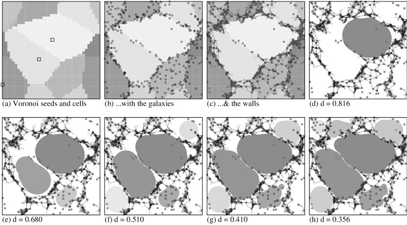
Figure 3: A demonstration of the way the void finder covers the voids. All panels depict the same slice, cut through a certain Voronoi tessellation. We present the Voronoi seeds ($\Box$) & cells (panel a), the galaxies (panel b) and the walls (panel c). The remaining panels show the voids’ image, at various void resolutions $d_{\tt i}$. More voids are recognized as we refine $d_{\tt i}$, and the older voids are enlarged.

Fig. 3 demonstrates how the void finder works. In all panels we show the same slice through a three-dimensional Voronoi Tessellation (see §4 for details), and we follow the development of the void image as we refine the void resolution. Initially, we locate the voids containing the largest empty spheres. In the following iterations we locate the smaller voids, and—when appropriate—enlarge the volumes of the older ones.

One must take into account the boundaries of the distribution. We treat the limits of the distribution as rigid boundaries. This may cause some distortion in the voids found close to the boundaries (causing them to be smaller than the rest). Still, this is the least speculative option as we do not make any assumptions about unsurveyed regions.

3.3 Statistical Significance

To assess the statistical significance of the voids we compare the voids found in observed data with voids found in equivalent random distributions. The random distributions mimic the sample’s geometry and density, and are analyzed by the algorithm in exactly the same manner. Averaging over the random catalogs we calculate $N_{\rm Poisson}(d)$, the expected number of voids in a Poisson distribution as a function of the void resolution $d$. We compare this with the observed number, $N_{\rm Survey}(d)$. We define the confidence level as:

$$p(d)=1-\frac{\mbox{$N_{\rm Poisson}(d)$}}{\mbox{$N_{\rm Survey}(d)$}}$$ (5)

The closer $p(d)$ is to unity, the less likely the void could appear in a random distribution. We consider voids with $p\geq 0.95$ as statistically significant. At a certain void resolution $d_{\rm stop}$, $N_{\rm Poisson}(d)$ exceeds $N_{\rm Survey}(d)$, and we terminate the void search.

The statistical significance defined in this way is attributed according to the order in which the voids were identified, not according to their sizes. This is so because the parameter determining how early a void is detected is the diameter of the largest sphere it contains, and not its total volume. Of course the total volume of a void and the diameter of the largest sphere contained in it are correlated. However, a void composed of a single large sphere will be detected earlier—and hence considered more significant—than a larger void composed of several spheres all having smaller radii. This is in agreement with the fact that clear spherical voids are more prominent when a galaxy distribution is inspected by eye. In retrospect this choice is also justified by the theoretical expectation that voids become more spherical with cosmological time (Blumenthal et al. 1992).

Voids in the actual surveys are systematically larger than the voids in the random distributions. When we reach the void resolution $d_{\rm stop}$ (where the number of voids in the random distributions exceeds the void number in the actual survey), the volume taken up by the random voids is still much smaller than the volume of the true voids. By ignoring this fact we actually under estimate the significance of the voids.

3.4 Redshift Surveys

The average galaxy number-density decreases with depth in a magnitude-limited redshift survey. If not corrected, this selection effect will interfere with the algorithm in the deeper regions of the sample: field galaxies will occur more frequently, and the derived size of the voids will be larger. Consequently, systematically larger voids will be found at greater distances.

To avoid these effects, one should use a volume-limited sample, in which the galaxy number-density is constant and independent of the distance. A volume-limited sample with $M\leq M_{o}$ has a depth:

$$\mbox{$r_{o}$}=\sqrt{\mbox{${\cal L}$}_{o}/4\pi\mbox{${\cal F}$}_{m_{b}}}=10^{-5-0.2(M_{o}-m_{b})}\,\mbox{Mpc}$$ (6)

where $m_{b}$ is the survey’s magnitude limit and $\mbox{${\cal L}$}_{o}$ is the luminosity that corresponds to $M_{o}$. However, current volume-limited samples are too small to study the LSS. For example, the SSRS2 sample contains 3162 galaxies with $r<130\mbox{$\>h^{-1}\>\mbox{Mpc}$}$. A volume-limited sample based on this distribution with such a depth ($M_{o}=-20.1$) retains only 528 galaxies. To overcome this, we use a semi–volume-limited sample: volume-limited up to some medium radius $r_{o}$, and magnitude-limited beyond. We choose the depth $r_{o}$ by maximizing the number of bright galaxies $N(M\leq M_{o})$:

$$N(M\leq M_{o})=\frac{4\pi}{3}\mbox{$r_{o}$}^{3}\cdot\eta\Gamma(1-\alpha,x_{o})$$ (7)

where $\eta$ is the galaxy number-density. The incomplete $\Gamma$-function arises from the integration of the appropriate Schechter function, with $x=\mbox{${\cal L}$}/\mbox{${\cal L}$}_{\star}$.

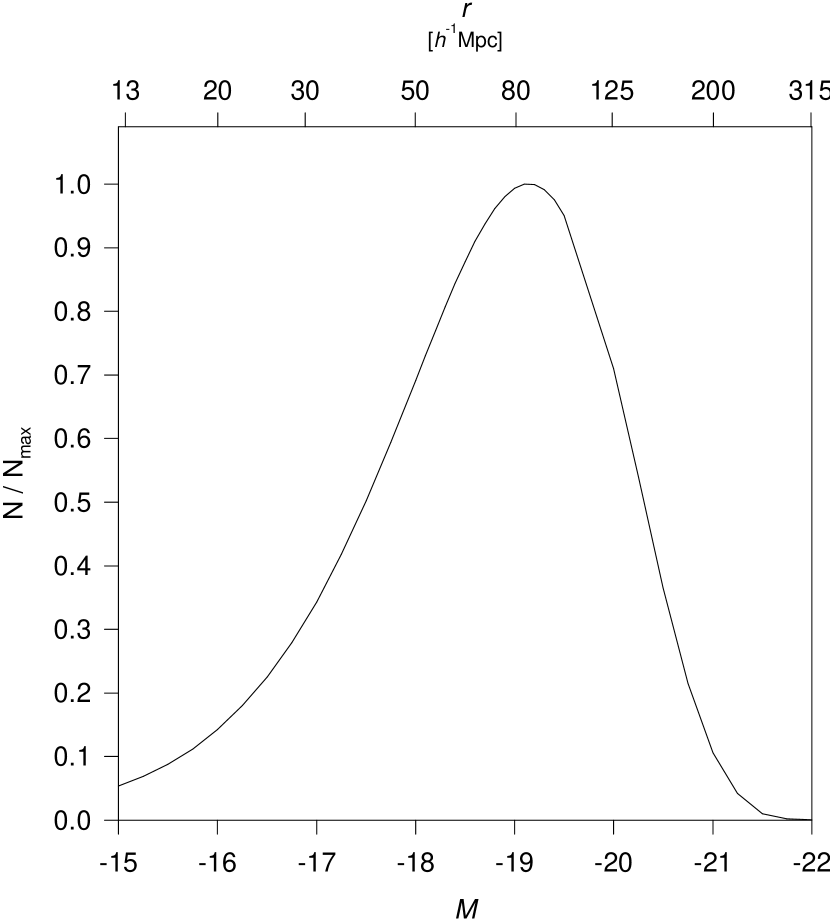
Figure 4: The relative number $N/N_{\mathrm{max}}$ in the SSRS2 sample ($m_{b}=15.5$, $\alpha=1.2$ and $M_{\star}=-19.5$) as a function of the depth of the volume-limited region. The number of galaxies $N$ peaks at $M=-19.1$ ($r=83\mbox{$\>h^{-1}\>\mbox{Mpc}$}$).

In Fig. 4 we plot the normalized $N(M_{o})$ for the SSRS2 parameters: $\alpha=1.2$, $M_{\star}=-19.5$ and $m_{b}=15.5$. In this example $N$ peaks close to $M_{\star}$ at $M=-19.1$, which corresponds to $x_{o}=0.69$ and a depth $\mbox{$r_{o}$}=83\mbox{$\>h^{-1}\>\mbox{Mpc}$}$. If we increase the depth of the volume-limited sample, the number of galaxies decreases.

No corrections are needed in the volume-limited region. We determine the values for $\ell$ and $d_{\tt i}$ in this region. Beyond $r_{o}$ we define $\phi(r)$, a selection-function based on the Schechter luminosity-function:

$$\phi(r)=\frac{\Gamma(1-\alpha,x_{M})}{\Gamma(1-\alpha,x_{M_{o}})}$$ (8)

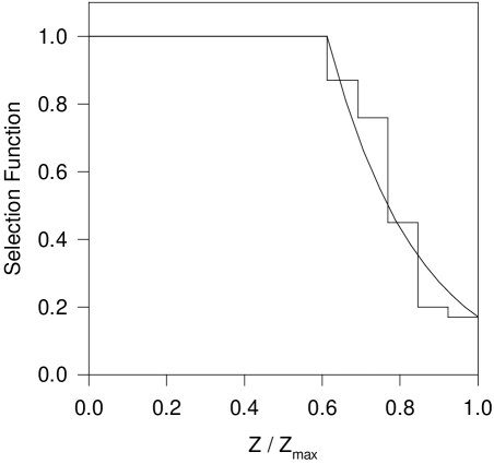
Figure 8: The SSRS2 selection-function, with $\mbox{$r_{o}$}=79.5\mbox{$\>h^{-1}\>\mbox{Mpc}$}$ and $\mbox{$r_{\rm max}$}=130\mbox{$\>h^{-1}\>\mbox{Mpc}$}$. The smooth line depicts $\phi$, where as the dashed line is the actual relative density, evaluated at 10$\>h^{-1}\>\mbox{Mpc}$ intervals.

where $x_{M}=10^{-0.4(M-M_{\star})}$. The selection-function $\phi(r)$ is the observed fraction of galaxies at the distance $r$, relative to $r_{o}$. A plot of the selection-function for the semi–volume-limited sample for SSRS2 is shown in Fig. 8. Using the selection-function, we modify both phases of the algorithm. In the wall builder phase, we consider larger spheres when counting neighbors at $r>\mbox{$r_{o}$}$. The radius of the counting-spheres is modified:

$$\ell^{\prime}=\left\{\begin{array}[]{ll}\ell&\mbox{if $r<\mbox{$r_{o}$}$}\\ \ell/\phi^{1/3}(r)&\mbox{otherwise}\end{array}\right.$$ (9)

A similar correction is applied to the void finder phase. A void of a given size found in a low density environment is less significant than a void of the same size found in a high density environment. In order that all the voids found in a given iteration are equally significant, we adjust the algorithm so that at a given iteration relatively larger voids are accepted, if located at $r>\mbox{$r_{o}$}$:

$$d^{\prime}_{\mathtt{i}}=\left\{\begin{array}[]{ll}d_{\mathtt{i}}&\mbox{if $r<\mbox{$r_{o}$}$}\\ d_{\mathtt{i}}/\phi^{1/3}(r)&\mbox{otherwise}\end{array}\right.$$ (10)

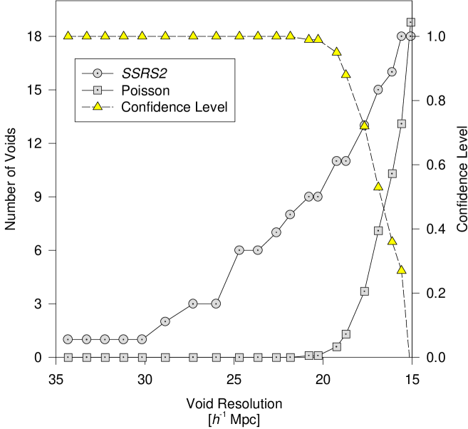
Figure 9: The accumulated number of voids as a function of the void resolution $d$, for the SSRS2 and for equivalent random catalogs. The derived confidence level $p$ is also indicated.

As mentioned earlier (§3.3), we use random distributions that mimic the true sample’s geometry and density, in order to assess the statistical significance of the voids. This scheme needs to be fitted, to correspond to the decrease in the galaxy density with $r$. We continue to use the same definition for the confidence level $p$ (eq. [5]). However, $d$ is now a function of $r$, scaled in the same manner given by equation (10) (see Fig. 9).

4 Voronoi Distributions

As a test-bed for the void finder algorithm, we use Voronoi distributions: A distribution of galaxies that is based on a Voronoi tessellation (Voronoi 1908). A Voronoi tessellation is a tiling of space into convex polyhedral cells, generated by a distribution of seeds. To generate a galaxy distribution in which the galaxies are located on the walls of the Voronoi cells, we have used an algorithm developed by Van de Weygaert & Icke (1989). The resultant galaxy distribution has the desired characteristic of large empty regions (i.e., voids), which we identify by the void finder algorithm.

A Voronoi tessellation is constructed from a given set of seeds $\{\vec{x}_{i}\}$. Based on the locations of these seeds, we divide the volume into cells. The Voronoi cell $\Pi_{i}$ of seed $i$ is defined by the following set of points $\vec{x}$:

$$\Pi_{i}=\{\>\vec{x}\;\;\>|\;\;\>{\mathrm{dist}}(\vec{x},\vec{x}_{i})<{\mathrm{dist}}(\vec{x},\vec{x}_{j})\quad\;\mbox{for all $j\neq i$}\>\}$$ (11)

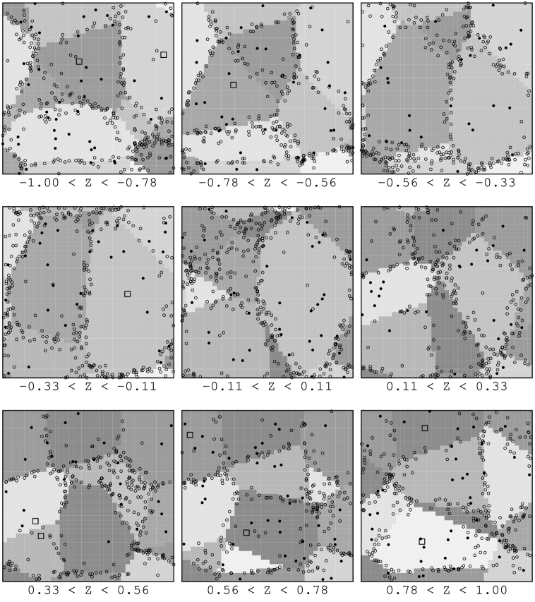
Figure 5: Nine planar slices showing Voronoi cells and galaxies in cubic Voronoi tessellation, generated from 10 seeds with 3000 galaxies (10% random). The cells are depicted using various shades of gray, indicating the intersection of the Voronoi cell with the plane at the center of the slab. The locations of the Voronoi seeds are marked by ‘$\Box$’. Galaxies associated with cell boundaries are marked by ‘$\circ$’, and random galaxies by ‘•’.

In other words, $\Pi_{i}$ is the set of points that is nearer to the seed $\vec{x}_{i}$ than to any other seed. In Fig. 5 we show two-dimensional cuts through a Voronoi tessellation.

We assign a finite width to the walls and position the galaxies on the boundaries between the Voronoi cells, with a Gaussian displacement in the distance from the exact cell boundary. These galaxies are designated to be wall galaxies, but do not necessarily end-up in this way: in regions where the galaxy distribution is sparse, the wall builder may identify these galaxies as field galaxies. Further still, if the galaxy density is low, there may be boundaries between Voronoi cells with no galaxies at all. Additional random galaxies correspond to field galaxies. Most of these randomly placed galaxies end-up as field galaxies. A few, located in dense areas, will be identified by the wall builder as wall galaxies.

We will call a galaxy distribution constructed in this way a Voronoi distribution. The location and number of the Voronoi cells (the would-be voids), the spread of the wall galaxies and the fraction of random galaxies are all known. Therefore, we can use this distribution as a test bed for our algorithm.

We have constructed a Voronoi distribution using 3000 galaxies and 10 seeds, which includes 300 (10%) random galaxies. These numbers correspond roughly to what is available in present redshift surveys. The original Voronoi tessellation (Fig. 5) is compared to the void finder reconstruction (Fig. 6). All Voronoi cells are reproduced except the very small cells near the boundaries, that were cut by the box limit. The reconstructed voids follow closely the original Voronoi cells, withstanding the noise introduced by the random galaxies. The walls highlighted using the wall builder are located along the boundaries between the Voronoi cells.

It is worthwhile to examine where the algorithm fails. A single void was broken into two (Fig. 6, lower-left corner of upper-left box) due to some random galaxies that extended the walls into this cell. Also note the instances where two Voronoi seeds are situated relatively close to each other (e.g., in the lower-left box). In such a situation the resultant wall is very sparse. This is due to the way in which the Voronoi code generates the galaxy distribution.

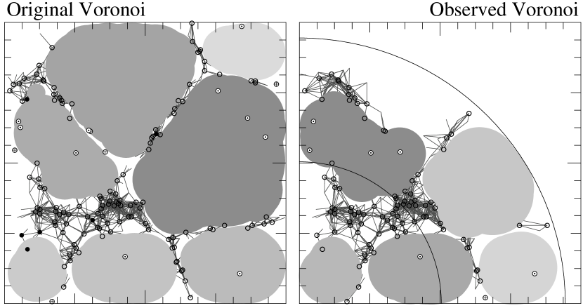
Figure 7: Left: void finder reconstruction of an ordinary Voronoi distribution. Right: reconstruction of a mock survey based on the same data. The intermediate arc marks the volume-limited region of the mock sample.

We have also created mock surveys, based on Voronoi distributions. Galaxies in the Voronoi distribution were assigned magnitudes according to a Schechter function. Then, a magnitude-limited sample was chosen. To this Voronoi-based mock survey we have applied our usual procedure: analyzing a semi–volume-limited sample, applying corrections beyond $r_{o}$. Fig. 7 shows a reconstruction based on the original data, along with a reconstruction based on the corresponding mock survey. The fit between the Voronoi cells and the recovered voids is still good, showing the adequacy of our method in analyzing actual surveys.

All together, the Voronoi tessellations that we examined show that the void finder indeed generates a faithful reproduction of the Voronoi cells. Further still, in cases where the reproduction merges adjacent Voronoi cells into one void, we see this as the adequate outcome of a missing wall. If we would have examined such a galaxy distribution by eye, with no prior knowledge about the locations of the Voronoi cells, we too would most likely consider that volume—originally occupied by two Voronoi cells—as one void. A level of $\sim 10\%$ random galaxies is tolerated, with no significant distortion in the void reproduction, and Voronoi-based mock surveys are also reproduced faithfully.

Boundary distortions are the cause for most of the cases in which the void finder departs from the original tessellation. This is also evident when considering the void volumes: The volume occupied by the voids is $\sim 15\%$ larger, if we consider only an inner cube and not the full tessellation. Voids near the boundaries are typically smaller (if at all recognized), as the Voronoi cells are bisected by the cube’s boundary.

5 Voids in the SSRS2

The SSRS2 survey (da Costa et al. 1994) consists of $\sim 3600$ galaxies with $m_{b}\leq 15.5$ in the region $-40\arcdeg<\delta<-2\fdg 5$ and $b\leq-40\arcdeg$, covering $1.13\,\mbox{sr}$. We have considered a semi–volume-limited sample, in this case consisting of galaxies brighter than $M_{o}\leq-19$, corresponding to a depth $\mbox{$r_{o}$}=79.5\mbox{$\>h^{-1}\>\mbox{Mpc}$}$. The Schechter luminosity function was evaluated with $M_{\star}=-19.5$ and $\alpha=1.2$, as derived for the SSRS2. Our final semi–volume-limited sample consists of 1898 galaxies, extending out to $\mbox{$r_{\rm max}$}=130\mbox{$\>h^{-1}\>\mbox{Mpc}$}$ where the selection-function $\phi$ has dropped to 17% (Fig. 8). It should be emphasized that the SSRS2 analysis is performed in redshift-space. However, because of the paucity of large clusters and the small amplitude of peculiar motions in the volume surveyed by the SSRS2, redshift distortions are small (da Costa et al. 1997) and the properties derived here should reflect those of voids in real-space.

The wall builder analysis of the SSRS2 has classified 1736 galaxies (91.5%) as wall galaxies, and 162 (8.5%) as field galaxies. The wall separation distance was $\ell=7.4\mbox{$\>h^{-1}\>\mbox{Mpc}$}$. In the volume-limited region we have $n^{-1/3}=6.4\mbox{$\>h^{-1}\>\mbox{Mpc}$}$, so $\ell/n^{-1/3}=1.16$. The wall galaxies are grouped in ten structures. The remarkable fact that one structure contains most (96%) of the wall galaxies will be discussed elsewhere, as this may have interesting statistical implications regarding the connectivity of the wall–filament skeleton. The rest of the wall galaxies are found in nine groups, each having 4 to 21 galaxies.

We have identified eleven significant ($p\geq 0.95$) voids within the volume probed by the SSRS2. These voids were detected while the void resolution was $d\geq 19.2\mbox{$\>h^{-1}\>\mbox{Mpc}$}$. In the following calculations we take into account only these voids, unless otherwise specified. Seven additional voids were identified before the void search was terminated at the resolution $\mbox{$d_{\rm stop}$}=15.1\mbox{$\>h^{-1}\>\mbox{Mpc}$}$, for which $p$ vanishes. Fig. 9 plots the accumulated number of voids in the SSRS2 and in the corresponding random catalogs, as a function of the void resolution $d$. The locations and characteristics of all eighteen voids are given in Table 1. Column (1) lists the confidence level $p$ attributed to each void. The diameters given in column (2) are of a sphere with the same volume as the whole void, as is listed in column (3). The center of the void given in columns (4)–(6) is defined as its center-of-(no)-mass. The density contrast value listed in column (7) was corrected for the average galaxy density at the same distance as the center of the void. In column (8) we give the fraction of the total volume of the void covered by the single largest sphere contained in it. This value is typically $\sim 40\%$ of the total volume of the void. Finally, in column (9) we indicate the corresponding voids identified in da Costa et al. (1988, hereafter dC88).

The average size of the voids in the survey as estimated from the equivalent diameters is $\bar{d}=40\pm 12\mbox{$\>h^{-1}\>\mbox{Mpc}$}$. The average under-density within the voids was found to be $\delta\rho/\rho\approx-0.9$, a quite remarkable result showing how empty voids are of bright galaxies. The eleven significant voids comprise 54% of the survey’s volume. An additional 5% is covered by the seven additional voids, totaling in $\sim 60\%$ of the volume being occupied by these voids. We estimate that the walls occupy less than 25% of the volume.

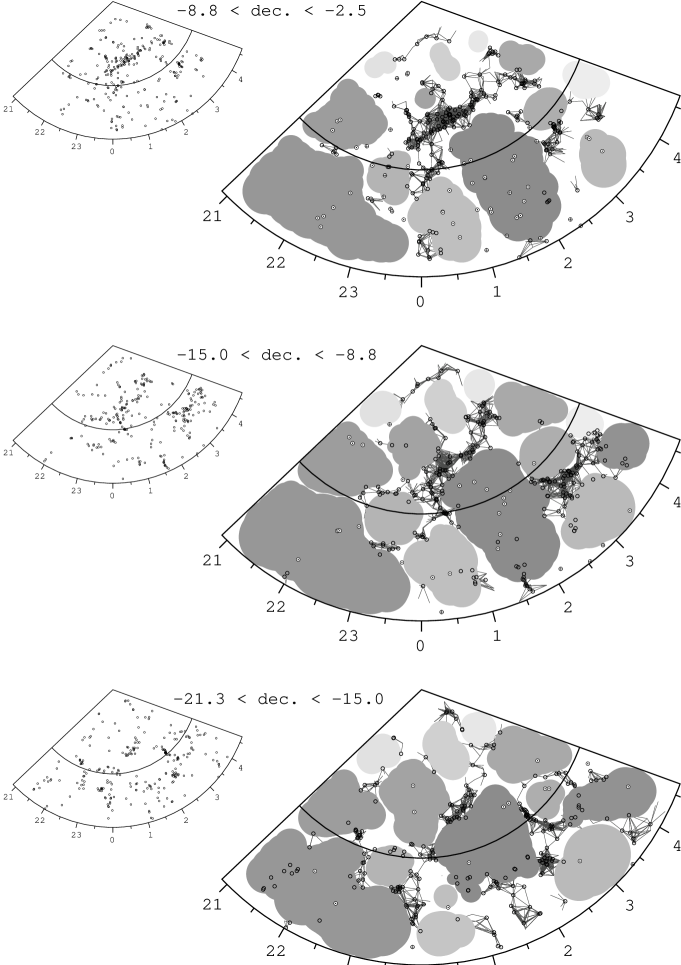
Figure 10: LSS in the SSRS2. The survey spans the declination range $-40\arcdeg<\delta<-2\fdg 5$, which we have split to six $6\fdg 25$-wide slices. Our sample extends to $\mbox{$r_{\rm max}$}=130\mbox{$\>h^{-1}\>\mbox{Mpc}$}$, and the intermediate arc marks $\mbox{$r_{o}$}=79.5\mbox{$\>h^{-1}\>\mbox{Mpc}$}$ (Continued on the following page).

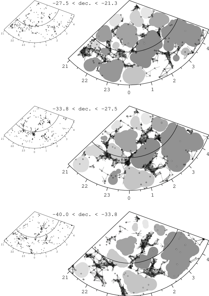
Figure 10: (Continued from previous page) Voids (grey areas), walls (dark lines) and galaxies (wall galaxies: ‘$\circ$’; void galaxies: ‘$\odot$’; field galaxies: ‘$\oplus$’).

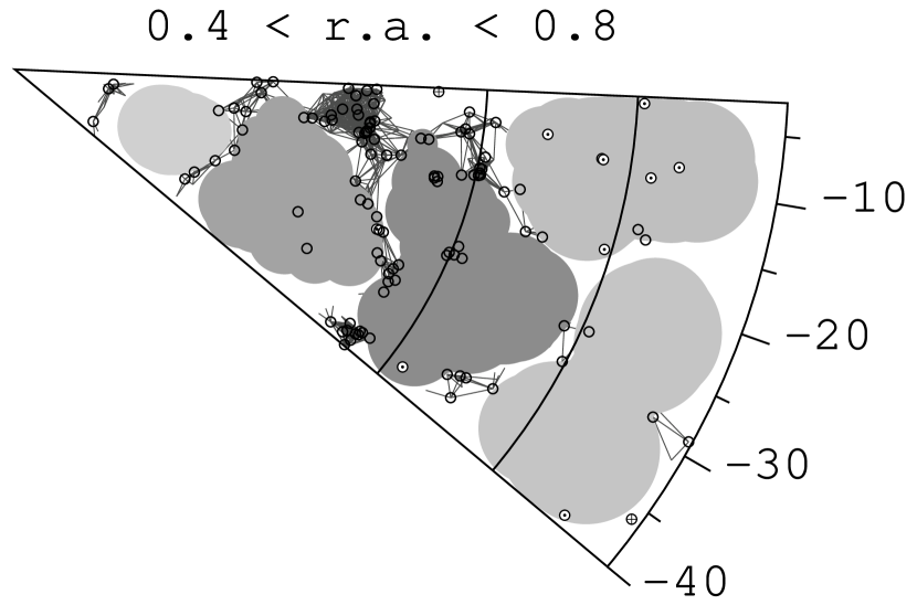
Figure 11: A constant right-ascension slice of the SSRS2, demonstrating the narrow ($37\fdg 5$) declination range of this survey. Most of the voids in this image are limited by the survey’s boundary.

The SSRS2 sample and the resultant void finder reconstruction is presented in Fig. 10, as six $6\fdg 25$-wide constant-declination slices. Do not be mislead by the wide right-ascension range of this survey, emphasized by these images. In declination the survey spans $37\fdg 5$ (see Fig. 11), limiting the sizes of the voids we find. The slices contain numerous walls and filaments. The nearest prominent features, the Fornax cluster and the Eridanus group, can easily be recognized at ($r\sim 10\mbox{$\>h^{-1}\>\mbox{Mpc}$},\alpha=3\fh 5$) running through most of the declination range. One of the outstanding structures in this survey is the Southern Wall (SW). This wall (dC88) is the dense structure running across all slices, from ($\alpha=4\mbox{${}^{\rm h}$}$, $r=45\mbox{$\>h^{-1}\>\mbox{Mpc}$}$) to ($\alpha=0\mbox{${}^{\rm h}$}$, $r=90\mbox{$\>h^{-1}\>\mbox{Mpc}$}$). It is especially prominent in the $\delta>-15\arcdeg$ and the $\delta<-27\fdg 5$ slices. The Pavo-Indus-Telescopium (PIT) supercluster runs along the line of sight at $\alpha=21\fh 5$ in the $\delta<-21\fdg 3$ slices. These two walls are almost parallel, and are connected through a third wall running perpendicular to the line of sight at $r\sim 90\mbox{$\>h^{-1}\>\mbox{Mpc}$}$ in the right ascension range $21\fh 5$ to $0\mbox{${}^{\rm h}$}$. These walls bound two voids (void 5 and void 12 in Table 1), identified earlier as one void (void 3 in dC88)—here the void is broken into two by a filament almost connecting PIT and the SW. A third structure runs parallel to the SW, bounding another void (void 1) between them.

The largest void found in the SSRS2 survey (void 3) has an equivalent diameter $d=60.8\mbox{$\>h^{-1}\>\mbox{Mpc}$}$, making it comparable in volume to the large void found in the Boötes (Kirshner et al. 1981). This void is an ellipsoid, whose major axis is perpendicular to the line of sight, located at: $80\mbox{$\>h^{-1}\>\mbox{Mpc}$}<r<130\mbox{$\>h^{-1}\>\mbox{Mpc}$}$; $-25\arcdeg<\delta<-2\fdg 5$; $21\mbox{${}^{\rm h}$}<\alpha<23\fh 75$. This void might actually be larger, since it is bounded (in three directions) by the limits of the SSRS2. A second large void (void 2, with $d=56.2\mbox{$\>h^{-1}\>\mbox{Mpc}$}$) is also comparable to the Boötes void.

When preparing the semi–volume-limited sample, we cast off all faint $M>M_{o}$ galaxies in the region $r<\mbox{$r_{o}$}$. These galaxies comprise the bulk of the surveyed galaxy population that we are forced to ignore (the rest are $r>\mbox{$r_{\rm max}$}$ galaxies, where the sample is too sparse). Although we cannot use these galaxies during the analysis phases, we can still try and benefit from them a posteriori: after the voids are located, we examine the locations of these galaxies. In this way we have divided the original galaxy distribution in the volume-limited region into two distinct populations, according to some absolute-brightness limit.

There are 1264 $M_{o}>-19$ galaxies in the volume-limited region of the SSRS2. Almost 61% of this region is covered by voids—but only 19% of the faint galaxies are found within them. Even though the void finder algorithm uses only the brighter galaxies in this region, we find that the faint galaxies do not fill the voids, providing an excellent verification of our algorithm. Still, the percentage of faint galaxies within the voids is significantly larger than that of the bright galaxies: only $\sim 5\%$ of the bright $M_{o}\leq-19$ galaxies are contained in the voids.

6 Discussion

We have used the void finder algorithm to analyze two redshift surveys: The SSRS2 and the IRAS 1.2 Jy survey (El-Ad, Piran & da Costa 1996b). These surveys represent two extreme cases in the trade-off between density and sky coverage. The SSRS2 is densely sampled ($m_{b}\leq 15.5$), but it has narrow angular limits, especially in the declination range. As a result, voids are often limited by the survey’s boundary, diminishing their scale. The IRAS is an almost full-sky survey ($87.6\%$ coverage), but it is rather sparse. As a result one cannot use a small void resolution, for lack of statistical significance. In addition to the above differences, the SSRS2 galaxies are optically selected, as opposed to the IRAS galaxies.

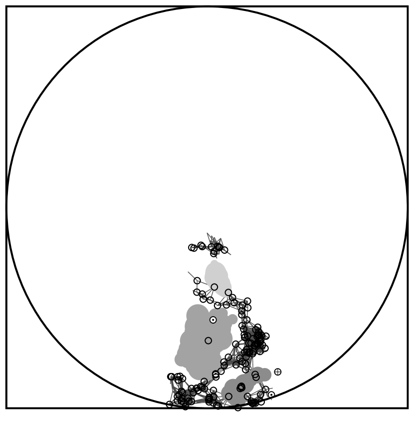
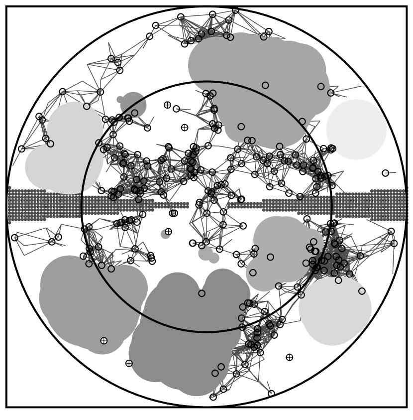
Figure 12: Voids in the SG plane: here we compare the redshift-space voids of the SSRS2 (left) and the IRAS (right). The denser sampling of the SSRS2 is evident. Similar voids are found in the overlapping regions of the two surveys.

Withstanding these differences, the results obtained with these surveys are similar. First, the surveys agree regarding individual voids in the regions where the surveys overlap. Fig. 12 depicts the redshift-space voids in the SG plane, for the IRAS and for the corresponding part of the SSRS2. In the region where the SSRS2 sample overlaps the IRAS sample, we find three of the eleven significant voids identified in the SSRS2. The corresponding IRAS voids are $\sim 33\%$ larger the SSRS2 ones, since they are not bounded by narrow angular limits as the SSRS2 voids.

Additionally, the results agree viz a viz the statistical characteristics of the voids:

1. Large voids occupy $\sim 50\%$ of the volume.

2. Walls occupy less than $\sim 25\%$ of the volume.

3. A void scale of at least 40$\>h^{-1}\>\mbox{Mpc}$, with an average under-density of $-0.9$.

4. Faint galaxies do not “fill the voids”, but they do populate them more than bright ones.

The void scale derived in both surveys is a lower limit: for the SSRS2, because of the narrow boundaries limiting the voids; and for the IRAS, due to the larger $d_{\rm stop}$, and because of the conservative analysis applied regarding the ZOA and the field galaxies. Further still, regarding the walls, both surveys poses the remarkable characteristic where almost all ($\sim 95\%$) of the wall galaxies are contained in a single structure.

The fact that both the IRAS and the SSRS2 are consistent regarding the void statistics as well as the individual voids is not trivial, since the IRAS galaxies represent a special galaxy class, which is biased relative to the optical galaxies (Lahav, Rowan-Robinson & Lynden-Bell 1988; Lahav, Nemiroff & Piran 1990). The agreement between the surveys suggests that a similar void scale exists for both optically and IRAS selected galaxies.

The IRAS data has been used to derive the smooth density field, and it probes a volume comparable to that used to determine the density field of the underlying mass distribution from the potent reconstruction method (Dekel, Bertschinger & Faber 1990) based on the measured galaxy peculiar velocity field. The voids and walls identified by our algorithm (El-Ad, Piran & da Costa 1996b) indeed correspond to the under-dense and over-dense regions in the IRAS density field (Strauss & Willick 1995) respectively. Comparison with the SFI sample (da Costa et al. 1996) also demonstrates that the voids delineated by galaxies correspond remarkably well with the under-dense regions in the reconstructed mass density field derived from peculiar velocity measurements (but also compare with the Mark III map—Dekel 1994; Dekel et al. 1997).

Most of the over-dense regions, walls and filaments, are narrower than 10$\>h^{-1}\>\mbox{Mpc}$. The smoothing scale used for creating the density fields spreads the originally thin structures over wider regions, extending into the under-dense volumes. This has the effect of giving a false impression of a rather blurred galaxy distribution, where prominent over-dense structures are separated by small under-dense regions. The true picture is very different: there is a sharp contrast between the thin over-dense structures which occupy only the lesser part of the volume, and the large voids. The notion of a void filled universe cannot be avoided in this picture.

We have developed and tested a new tool for quantifying the large-scale structure of the universe. We focus on the under-dense regions, and for the first time we have individually identified and statistically quantified the voids. The void finder analysis clearly shows the prominence of the voids in the LSS, not hindered by smoothing of the over-dense regions, and it reveals the image of a void-filled universe, where large voids are a common feature.

The consistency in the void image between IRAS and optically selected galaxies suggests that galaxies of different types delineate equally well the observed voids. Therefore galaxy biasing is an unlikely mechanism for explaining the observed voids in redshift surveys. Comparison with the recovered mass distribution further suggests that the observed voids in the galaxy distribution correspond well to under-dense regions in the mass distribution. This confirms the gravitational origin of the voids (Piran et al. 1993).

	Confidence	Equivalent	Total	Location of Center			Void	Largest
	Level	Diameter	Volume	(Equatorial Coordinates)			Under-	Sphere’s
	$p$	[$\>h^{-1}\>\mbox{Mpc}$]	[$h^{-3}\>\mbox{KMpc}^{3}$]	$r$	$\alpha$	$\delta$	density	Fraction	Identification
	(1)	(2)	(3)	(4)	(5)	(6)	(7)	(8)	(9)
1	$>$0.99	54.3	084.9	085.7	$1\mbox{${}^{\rm h}$}33\mbox{${}^{\rm m}$}$	$-16\arcdeg 45\arcmin$	-0.89	0.25
2	$>$0.99	56.2	093.9	099.7	$3\phantom{\mbox{${}^{\rm h}$}}34\phantom{\mbox{${}^{\rm m}$}}$	$-28\phantom{\arcdeg}50\phantom{\arcmin}$	-0.87	0.20	dC88 void 4
3	$>$0.99	60.8	119.0	107.2	$22\phantom{\mbox{${}^{\rm h}$}}25\phantom{\mbox{${}^{\rm m}$}}$	$-14\phantom{\arcdeg}46\phantom{\arcmin}$	-0.93	0.25
4	$>$0.99	35.6	024.0	066.7	$21\phantom{\mbox{${}^{\rm h}$}}43\phantom{\mbox{${}^{\rm m}$}}$	$-14\phantom{\arcdeg}40\phantom{\arcmin}$	-0.91	0.37
5	$>$0.99	34.8	022.6	053.0	$23\phantom{\mbox{${}^{\rm h}$}}48\phantom{\mbox{${}^{\rm m}$}}$	$-24\phantom{\arcdeg}39\phantom{\arcmin}$	-0.94	0.39	dC88 void 3 (Sculptor)
6	$>$0.99	32.0	017.4	056.5	$3\phantom{\mbox{${}^{\rm h}$}}56\phantom{\mbox{${}^{\rm m}$}}$	$-20\phantom{\arcdeg}11\phantom{\arcmin}$	-0.92	0.47
7	$>$0.99	25.5	008.8	077.2	$3\phantom{\mbox{${}^{\rm h}$}}17\phantom{\mbox{${}^{\rm m}$}}$	$-11\phantom{\arcdeg}40\phantom{\arcmin}$	-0.91	0.71
8	$>$0.99	27.8	011.4	083.9	$23\phantom{\mbox{${}^{\rm h}$}}20\phantom{\mbox{${}^{\rm m}$}}$	$-12\phantom{\arcdeg}32\phantom{\arcmin}$	-0.95	0.59
9	0.99	39.0	031.1	114.6	$3\phantom{\mbox{${}^{\rm h}$}}06\phantom{\mbox{${}^{\rm m}$}}$	$-13\phantom{\arcdeg}47\phantom{\arcmin}$	-0.86	0.54
10	0.95	34.8	022.4	104.7	$0\phantom{\mbox{${}^{\rm h}$}}26\phantom{\mbox{${}^{\rm m}$}}$	$-9\phantom{\arcdeg}17\phantom{\arcmin}$	-0.69	0.39
11	0.95	42.9	041.5	112.8	$0\phantom{\mbox{${}^{\rm h}$}}21\phantom{\mbox{${}^{\rm m}$}}$	$-29\phantom{\arcdeg}43\phantom{\arcmin}$	-0.88	0.31
12	0.72	25.0	008.1	074.8	$23\mbox{${}^{\rm h}$}03\mbox{${}^{\rm m}$}$	$-32\arcdeg 35\arcmin$	-0.97	0.37
13	0.72	22.1	005.8	031.0	$1\phantom{\mbox{${}^{\rm h}$}}23\phantom{\mbox{${}^{\rm m}$}}$	$-19\phantom{\arcdeg}36\phantom{\arcmin}$	-1.00	0.55	dC88 void 1
14	0.53	21.3	005.2	087.2	$21\phantom{\mbox{${}^{\rm h}$}}28\phantom{\mbox{${}^{\rm m}$}}$	$-29\phantom{\arcdeg}28\phantom{\arcmin}$	-1.00	0.62
15	0.53	27.3	010.7	116.1	$21\phantom{\mbox{${}^{\rm h}$}}24\phantom{\mbox{${}^{\rm m}$}}$	$-33\phantom{\arcdeg}17\phantom{\arcmin}$	-0.74	0.86
16	0.36	20.3	004.4	036.5	$21\phantom{\mbox{${}^{\rm h}$}}43\phantom{\mbox{${}^{\rm m}$}}$	$-18\phantom{\arcdeg}41\phantom{\arcmin}$	-1.00	0.52
17	0.27	19.0	003.7	032.1	$3\phantom{\mbox{${}^{\rm h}$}}42\phantom{\mbox{${}^{\rm m}$}}$	$-21\phantom{\arcdeg}21\phantom{\arcmin}$	-1.00	0.62
18	0.27	21.1	004.9	085.9	$4\phantom{\mbox{${}^{\rm h}$}}18\phantom{\mbox{${}^{\rm m}$}}$	$-8\phantom{\arcdeg}42\phantom{\arcmin}$	-1.00	0.50

Table 1: Locations & properties of the voids in the SSRS2 survey.

Figure 1: Wall construction using the wall builder. Panel a: A toy distribution of 16 galaxies ($\circ$). Panel b: After the calculation of $\ell$, all galaxy pairs closer than this separation are marked. Panel c: Galaxies with less than three neighbors are flagged as field galaxies ($\oplus$). Panel d: The final result (after one additional iteration of neighbors count). The string extending between the dense structures has been eliminated.