ANISOTROPIES IN THE COSMIC MICROWAVE BACKGROUND: THEORY

Anisotropies in the Cosmic Microwave Background (CMB) contain a wealth of information about the past history of the universe and the present values of cosmological parameters. I ouline some of the theoretical advances of the last few years. In particular, I emphasize that for a wide class of cosmological models, theorists can accurately calculate the spectrum to better than a percent. The specturm of anisotropies today is directly related to the pattern of inhomogeneities present at the time of recombination. This recognition leads to a powerful argument that will enable us to distinguish inflationary models from other models of structure formation. If the inflationary models turn out to be correct, the free parameters in these models will be determined to unprecedented accuracy by the upcoming satellite missions.

1 History

The Texas Symposium on Relativistic Astrophysics was held in Chicago ten years ago in 1986. David Wilkinson spoke about the cosmic microwave background. He undoubtedly made the point that the CMB provides us with some of the best evidence for the Big Bang. There was no evidence (and there still is no evidence) for any deviations from a black-body spectrum. And this is one of the primary predictions of the Big Bang.

Wilkinson devoted most of his talk to searches for anisotropies in the CMB. The fact that the CMB temperature is the same in all directions indicates that the universe was very smooth early in its history. However, cosmologists generally work within the framework of gravitational instability which says that small inhomogeneities early on grew via gravity into the large structures we see today. Thus, the CMB should not be perfectly isotropic; it should carry some imprint of those small, early inhomogeneities. Wilkinson compiled the upper limits on anisotropies from the experiments of the time. This compilation is reproduced in Figure 1, where I have taken the liberty of slightly changing his notation. In particular, it is convenient to expand the temperature on the sky in terms of spherical harmonics

$${T(\theta,\phi)\over T_{0}}=\sum_{l=0}^{\infty}\sum_{m=-l}^{l}a_{lm}Y_{lm}(\theta,\phi).$$ (1)

When we expand in this fashion, low $l$’s correspond to anisotropies on large angular scales (the quadrupole is $l=2$) while large $l$’s correspond to anisotropies on small scales. The square of the coeffients of the $Y_{lm}$’s are known as the $C_{l}$’s. These are extremely useful things becuase they can be calculated by theorists and measured by observers. A given experiment at angular scale $l$ measures $\delta T_{rms}\sim[l(l+1)C_{l}/2\pi]^{1/2}$. The upper limits at the time correspond to $\delta T_{rms}\sim 50-200\mu$K.

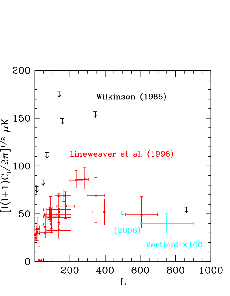
Figure 1: Observations of the CMB spectrum. Upper limits are those compiled by Wilkinson in 1986. Detections were compiled by Lineweaver based on results within the last two years. Anticipated error bars from satellites are also shown.

Wilkinson was obviously aware of the fact that these upper limits were tantalizingly close to the levels of anisotropies predicted by many theories. He ended his talk by saying, “If the anisotropies are indeed just below current limits, as most of us feel they must be, the next few years should see this field turn from one of searching to one of studying.”

2 Experiments

How has the field progressed since Wilkinson’s review? Figure 1 shows, along with Wilkinson’s compilation, a recent compilation$\!{}^{{\bf?}}$ of all experiments in the last two years. Starting with the COBE$\!{}^{{\bf?}}$ detection in 1992 at the largest angular scales, there have been dozens of detections on a wide range of angular scales. These detections, as Wilkinson’s quote makes clear, were anticipated based on typical models of structure formation. Although the details are not yet in, it is safe to say that gravitational instability theories predicted the level of anisotropies that are observed today.

Another feature of the detections is just now becoming evident. As one moves from low $l$ to high $l$ (from large scales to small scales), one sees evidence of a gradual rise in the the amplitude of the anisotropies. We will see shortly that this too is a prediction of some of the more popular models of structure formation.

How will the situation look ten years from now when results from the current crop of balloon-borne and ground-based experiments have come in, and the two satellite experiments (MAP$\!{}^{{\bf?}}$ and PLANCK$\!{}^{{\bf?}}$) will have made all-sky maps? Figure 1 shows the expected error bars in the year 2006. There are several ways to represent the knowledge we will have at the time. First, it is important to note that, today, experiments are sensitive to a range of $l$’s: thus, $C_{500}$ for example is not measured by a given small scale experiment. Rather, each experiment measures a signal integrated over a wide range of $l$. This range is depicted by the horizontal error bars in Figure 1. In the future, we can continue to smooth over the $l$’s in this fashion. Then the errors will be as shown on the far right in Figure 1. In order to see them on this graph, I have blown them up by a factor of 100! We will also have the ability by then, though, to determine each individual $C_{l}$. The expected errors on $C_{500}$ are shown in Figure 1. Either way you look at it, we will have an extraordinary amount of information in ten years. For the experimentalists, at least, it is clear that Wilkinson’s prediction has come true. The field really has moved from searching to studying.

3 Theory

CMB theorists have also been very active over the last few years. First of all, for a wide range of models, we are confident that we can calculate$\!{}^{{\bf?}}$ the anisotropy spectra – the $C_{l}$’s – to an accuracy of better than a percent. Figure 2 shows the results of seven different groups who independently calculated the $C_{l}$’s for a given model. This graph was made about two years ago, and the agreement has only gotten better since then. Not only can we calculate accurately, but we can also calculate quickly. Thanks to Seljak and Zaldariagga$\!{}^{{\bf?}}$, in the time it has taken me to write this paragraph, we could have run off another set of $C_{l}$’s.

Figure 2: Seven different calculations of the CMB power spectrum for a model with adiabatic fluctuations. All lie within the shaded band which illustrates the minimum “cosmic variance” errors.

We also have made great strides in the last few years understanding the bumps and wiggles in the theoretical curves. To understand the structure of these anisotropies, we need to review the thermal history of the universe. Recall that, early in the history of the universe, the temperature of the cosmic gas was very high. So, anytime a free electron and proton came together to form a hydrogen atom, a high energy photon immediately destroyed it. There was essentially no neutral hydrogen early on. This situation changed dramatically when the temperature dropped below $1/3$ eV. After that time, there were not enough ionizing photons around. So almost all the free electrons and protons combined into neutral hydrogen. This had dramatic implications for the cosmic photons. As long as the electrons were free, they interacted with the photons via Compton scattering. After they combined into hydrogen, the photons travelled freely from the “surface of last scattering” to us today. So, for the purposes of the CMB, the universe is neatly divided into two epochs: Before Recombination when the photons and electrons behaved as a tightly coupled fluid and After Recombination when photons freestreamed. The mathematics of freestreaming is a little complicated, but the physics is completely trivial: it just requires us to trace the paths of free photons. So the physics behind the spectrum of anisotropies comes solely from the epoch Before Recombination.

It pays to reiterate that Before Recombination, the photons and electrons acted as a fluid. By this, I mean that it could be described by only its $l=0$ component (as opposed to all the multipole moments that are needed to describe it today). This represents an immense simplification: instead of solving a infinite heirarchy of coupled differential equations for all the photon moments, we need solve for only one of the moments. The forces acting on this moment, let’s call it $\delta T$, are pressure and gravity. These forces act in opposite directions. Pressure tends to smooth out any inhomogeneities (i.e. drives $\delta T$ to zero) while gravity produces inhomogeneities. It is not surprising then that acoustic oscillations are set up in the medium. In fact, Hu & Sugiyama$\!{}^{{\bf?}}$ have shown that this oscillation pattern is precisely the one imprinted in the $C_{l}$ spectrum of Figure 2. A quantitative analysis shows that there are two possible modes that can be excited in this fluid. In particular,

$$\delta T(\vec{x},\eta)=\int d^{3}ke^{i\vec{k}\cdot\vec{x}}\left[A\cos[k\eta/{\sqrt{3}}]+B\sin[k\eta/{\sqrt{3}}]\right]$$ (2)

where $\eta$ is conformal time. Again, not surprisingly, the $C_{l}$ spectrum today is radically different if the sine mode is excited than if the cosine mode is excited. Figure 3 shows that, as you would expect, the spectra are out of phase with each other.

Figure 3: The power for two different theories, one of which (adiabatic) excites the cosine mode of acoustic oscillations the other (isocurvature) the sine mode. Inflationary predictions typically look like the adiabatic spectrum here. Defect models should have some of the features of the isocurvature spectrum, but the calculations at present are not yet believable.

It is clear from the present data shown in Figure 1 that we will shortly be able to tell which of the two theoretical curves in Figure 3 is more accurate. That is, we will soon know whether the sine or the cosine mode were excited in the early universe. This is extremely important because we expect the two most popular mechanisms of structure formation – inflation and topological defects – to excite different modes. Let me walk through this argument which has recently been clearly elucidated by Hu & White$\!{}^{{\bf?}}$. Any theory which respects causality necessarily requires that there be no correlations on very large scales (scales that have not been in causal contact with each other). This is equivalent to a boundary condition on $\delta T$; namely that the Fourier transform vanishes at $k=0$. This means that only $B$ in equation 2 can be non-zero. So topological defects, which of course obey causality, can be expected to excite the sine mode. Inflation is a theory which introduces correlations amongst scales that appear to be causally disconnected. Thus, inflationary models can, and most often do, excite the cosine mode.

Figure 4: The spectra for adiabatic models with different sets of parameters. Varied are the cosmological constant, neutrino mass, spectral index, and Hubble constant.

There are several caveats to the above argument. First of all, the predictions for the adiabatic models depend on various cosmological parameters$\!{}^{{\bf?}}$: the slope of the primordial spectrum, the contribution from tensor modes, the Hubble constant, the baryon density, and several others. Thus the actual curves share some of the features of the curve labelled “Adiabatic” in figure 3, but the predictions are by no means unique (see figure 4). Fortunately there are some robust features of these curves which hold up even after allowing many parameters to vary. The second caveat is that we simply do not know for sure that defect theories follow the general isocurvature model. There have been a few calculations of the spectrum in defect models$\!{}^{{\bf?}}$. As one who is actively at work on one such calculation, I think it is fair to say that we have not yet reached agreement.

Assuming there are no major theoretical surprises, we can expect the experiments over the next several years to pick out whether toppological defects or inflation are correct. Once that issue is settled, it remains to pin down the cosmological parameters which impact upon the spectrum. One might think that since there are so many free parameters, they cannot all be determined simultaneously. Recent work has shown that this is not true. Figure 5 shows an example$\!{}^{{\bf?}}$: we let five parameters vary and show the error ellipses projected down onto a couple of two dimensional planes. The top figure shows that it is quite possible that by the year 2006, we will not be arguing about whether the Hubble constant is $50$ or $100$, but rather whether it is $50.5$ or $50.0$. The bottom figure shows that, in addition to the cosmological parameters, we should get a good handle on the inflationary parameters, thereby allowing us to distinguish amongst different inflationary models$\!{}^{{\bf?}}$. A number of groups$\!{}^{{\bf?}}$ have varied even more parameters and all have reached the same general conclusion: the cosmological parameters will be pinned down to unprecedented accuracy by the satellite experiments.

Figure 5: The estimated 95% contours for the MAP (larger ellipses in each case) and PLANCK (formerly COBRAS/SAMBA) satellites. In each case five variables – the amplitude of the scalar and tensor perturbations, the spectral index of the scalars, the baryon density, and the Hubble constant – are allowed to vary. The ellipses are the projections of the five dimensional ellipses onto the (Hubble constant,Baryon density) plane and the (spectral index,tensor/scalar ratio) plane. The points and lines in the $n-r$ plane correspond to the predictions of different inflationary models.

4 Conclusions

About thirty years ago, Penzias and Wilson discovered the cosmic microwave radiation. This discovery convinced the vast majority of physicists that the Big Bang model was correct. In 1992, the COBE satellite discovered anisotropies in the CMB. The existence and amplitude of these anisotropies were predicted by theories which relied on gravitational instability to form structure. It is perhaps too early to know for sure, but I would guess that COBE’s most enduring legacy will be its evidence that current models of structure formation are on the right track.

A number of cosmologists are beginning to speculate about what we will have learned in ten years after the next generation of balloon and ground based experiments and after the MAP and PLANCK satellites have flown. There is a very good chance these measurements will clearly distinguish between the two most popular models of structure formation: inflation and topological defects. Indeed, this could happen very soon. If a peak does indeed develop in the $C_{l}$ spectrum at around $l\sim 200$, this will be strong evidence for inflation. If the general picture of inflation is verified in this manner, the fun will begin. It will then be possible to determine many of the cosmological parameters to unprecedented accuracy. Further, the experiments will contain so much information that it will be possible to distinguish amongst different inflationary models. This opens a window to study physics at energies that are twelve orders of magnitude higher than those probed by the largest accelerators.

Many people are fond of pointing out that something completely unexpected and confusing may turn up, thereby upsetting the possibility of any such determinations. Of course this is possible. Unexpected and confusing discoveries have rocked cosmology for decades. The “man-bites-dog” story in cosmology though is the one in which the confusion ends; this may well happen within the next ten years.

References

References

- [1] C. H. Lineweaver et al, astro-ph/9610133.
- [2] G.P. Smoot et al, Astrophys. J. 396, L1 (1992).
- [3] The MAP home page is http://map.gsfc.nasa.gov/.
- [4] The PLANCK (formerly COBRAS/SAMBA) home page is http://astro.estec.esa.nl/SA-general/Projects/Cobras/cobras.html.
- [5] P.J.E. Peebles and J.T. Yu, Astrophys. J. 162, 815 (1970); M.L. Wilson and J. Silk, Astrophys. J. 243, 14 (1981); J.R. Bond and G. Efstathiou, Astrophys. J. 285, L45 (1984).
- [6] U. Seljak and M. Zaldariagga, Astrophys. J. 469, 437 (1996).
- [7] W. Hu and N. Sugiyama, Astrophys. J. 444, 489 (1995); F. Atrio-Barandela and A. G. Doroshkevich, Astrophys. J. 420, 26 (1994); P. Nasel’skij and I. Novikov, Astrophys. J. 413, 14 (1993); U. Seljak, Astrophys. J. 435, L87 (1994); A. G. Doroshkevich. Ya. B. Zeldovich, and R. A. Sunyaev, Sov. Astron. 22, 523 (1978); A. G. Doroshkevich, Sov. Astron. Lett. 14, 125 (1988).
- [8] W. Hu and M. White, Phys. Rev. Lett. 77, 1687 (1996); N. G. Turok, astro-ph/9607109 (1996).
- [9] J. R. Bond, R. Crittenden, R. L. Davis, G. Efstathiou and P. J. Steinhardt, Phys. Rev. Lett. 72, 13 (1994).
- [10] R. G. Crittenden and N. G. Turok, Phys. Rev. Lett. 75, 2642 (1995); A. Albrecht, D. Coulson, P. Ferreira, and J. Magueijo, Phys. Rev. Lett. 76, 1413 (1996).
- [11] S. Dodelson, W. Kinney, and E. W. Kolb, (1997).
- [12] L. Knox and M. S. Turner, Phys. Rev. Lett. 73, 3347 (1994).
- [13] L. Knox, Phys. Rev. D52, 4307 (1995); G. Jungman, M. Kamionkowski, A. Kosowsky , and D. N. Spergel, Phys. Rev. D54, 1332 (1996); S. Dodelson, E. I. Gates, and A. S. Stebbins, Astrophys. J. 467, 10 (1996).