Dynamical Modeling of Velocity Profiles:
The Dark Halo Around the Elliptical Galaxy NGC 2434

Abstract

We describe a powerful technique to model and interpret the stellar line-of-sight velocity profiles of galaxies. It is based on Schwarzschild’s approach to build fully general dynamical models. A representative library of orbits is calculated in a given potential, and the non-negative superposition of these orbits is determined that best fits a given set of observational constraints. Our implementation incorporates several new features: (i) we calculate velocity profiles and represent them by a Gauss-Hermite series. This allows us to constrain the orbital anisotropy in the fit. (ii) we take into account the error on each observational constraint to obtain an objective $\chi^{2}$ measure for the quality-of-fit. Given the observational constraints, the technique assesses the relative likelihood of different orbit combinations in a given potential, and of models with different potentials. In our implementation only projected, observable quantities are included in the fit, aperture binning and seeing convolution of the data are properly taken into account, and smoothness of the models in phase-space can be enforced through regularization. This scheme is valid for any geometry.

In a first application of this method, we focus here on spherical geometry; axisymmetric modeling is described in companion papers by Cretton et al. and van der Marel et al. We test the scheme on pseudo-data drawn from an isotropic Hernquist model, and then apply it to the issue of dark halos around elliptical galaxies. We model radially extended stellar kinematical data for the E0 galaxy NGC 2434, obtained by Carollo et al.  Constant mass-to-light ratio models are clearly ruled out, regardless of the orbital anisotropy. To study the amount of dark matter needed to match the data, we considered a sequence of cosmologically motivated ‘star+halo’ potentials. These potentials are based on the CDM simulations by Navarro et al., but also account for the accumulation of baryonic matter; they are specified by the stellar mass-to-light ratio $\Upsilon_{*,B}$ and the characteristic halo velocity, $V_{200}$. The star+halo models provide an excellent fit to the data, with $\Upsilon_{*,B}=3.35\pm 0.25$ (in B-band solar units) and $V_{200}=450\pm 100$ km/s. The best-fitting potential has a circular velocity $V_{\rm c}$ that is constant to within $\sim 10\%$ between $0.2$–3 effective radii and is very similar to the best-fitting logarithmic potential, which has $V_{\rm c}=300\pm 15{\rm\,km\,s^{-1}}$. In NGC 2434 roughly half of the mass within an effective radius is dark. Models without a dark halo overestimate the mass-to-light ratio of the stellar population by a factor of $\sim 2$.

1 Introduction

Mapping how the ratio of luminous to dark matter in a galaxy changes as a function of radius provides an important test for galaxy formation scenarios. Numerical simulations of halo formation in a cosmological context have reached a level where they can predict the radial profile of an isolated dark halo (Navarro et al. 1996, hereafter NFW; Cole & Lacey 1996). This profile is altered by the presence of dissipative, baryonic matter, which collects at the center and contracts the dark matter profile. This contraction may provide a natural explanation for the observed fact that the circular velocity is approximately constant with radius in spiral galaxies (Blumenthal et al. 1986; NFW). Elliptical galaxies are more centrally concentrated than spiral galaxies of the same mass, suggesting that they may have circular velocities that are higher in the inner parts than in the outer parts.

Observational studies of the dark halos in spiral galaxies (e.g., van Albada et al. 1985) are comparably straightforward. HI gas provides an excellent tracer to large radii. To interpret the kinematics it is justifiable to assume a nearly co-planar distribution with nearly circular orbits, upon which the gravitational potential can be constrained from the observables. By contrast, the majority of elliptical galaxies do not have HI disks that are in equilibrium, and the transition from where the stellar mass dominates to where the dark halo dominates has remained poorly constrained. This has been due to the difficulties in obtaining unambiguous results from the stellar kinematics, as caused by two main problems. First, modeling the stellar dynamics for ellipticals is much more complex than for the cold disks of spirals (e.g., de Zeeuw & Franx 1991; Bertin & Stiavelli 1993; de Zeeuw 1996). Random motions dominate, and the stars can occupy a host of qualitatively different orbits in any given potential. Hence, the dynamical modeling must solve for both the potential and the orbital distribution of the stars, given the observed projected positions and velocities of stars. In practice, most existing studies have not done this. Instead, the orbital structure has often been assumed a priori, by requiring that the distribution function (hereafter, DF; i.e., the number of stars per unit volume of the phase space of stellar positions and velocities) has a certain simple form. The second reason for the poor understanding of the star–halo connection in ellipticals has been the fact that until recently good stellar kinematic data were available only out to approximately one effective radius $R_{\rm eff}$. This left more than half the stellar mass kinematically unconstrained. In addition, the data were generally restricted to measurements of the two lowest order velocity moments, i.e., the mean streaming velocity $V$ and the line-of-sight velocity dispersion $\sigma$. These quantities contain no or little independent information on the intrinsic velocity dispersion anisotropy of the system (Binney & Mamon 1982), which provides the main indeterminacy in the modeling. As a consequence, stellar dynamical indications for the presence of dark halos around elliptical galaxies have remained ambiguous. There have been indications for dark halos in studies that employed restricted classes of dynamical models (e.g., van der Marel 1991; Saglia et al. 1992). However, the few models in the literature that had the full freedom of rearranging orbits (e.g., Richstone & Tremaine 1984; Dejonghe 1989) have been able to fit the data for most ellipticals without requiring any dark matter (Katz & Richstone 1985; Saglia et al. 1993; Bertin et al. 1994). Discrete kinematical tracers in elliptical galaxies (i.e., planetary nebulae and globular clusters) have the advantage that they can be observed to larger radii, but they have the disadvantage of small-number statistics. Dynamical modeling of their observed radial velocities is beset by the same degeneracies that plague the interpretation of the integrated light measurements. Not surprisingly, these studies have produced similarly ambiguous results (e.g., Ciardullo, Jacoby & Dejonghe 1993; Tremblay, Merritt & Williams 1995). Yet, as summarized in various reviews (e.g., Ashman 1992; de Zeeuw 1995; Saglia 1996), there is independent evidence for extended dark matter from X-ray measurements of luminous galaxies (e.g., Forman, Jones & Tucker 1985; Awaki et al. 1994), from HI kinematics (Franx et al. 1994), and from gravitational lensing (e.g., Maoz & Rix 1993; Kochanek 1995). It is likely that this apparent discrepancy is attributable to the shortcomings of the stellar dynamical tests, i.e., to the uncertainty about the orbital distributions resulting from insufficiently constraining data.

There are several reasons for being optimistic that this situation can be improved and that the luminous to dark matter distribution in elliptical galaxies can now be investigated in some detail through stellar dynamical studies. First, improved CCD technology (larger detector size, higher QE, lower read-out noise and dark current), combined with improved strategies to ensure accurate sky subtraction and better stellar template matching, have made it possible to obtain stellar kinematics to 2–4 $R_{\rm eff}$ (Carollo et al. 1995, hereafter C95; Statler et al. 1996). With data reaching out to these radii, kinematic constraints can be obtained over most of the stellar body. Second, improved analysis techniques (e.g., Rix & White 1992; van der Marel & Franx 1993, hereafter vdMF; Kuijken & Merrifield 1993) make it possible now to extract the entire line-of-sight velocity profile (VP) from the absorption-line spectra, rather than only its lowest order moments $V$ and $\sigma$. The higher moments of the VP, which can now be measured, contain essential information about the anisotropy of the velocity distribution (e.g., Dejonghe, 1987; Gerhard 1993; C95).

The main purpose of this paper is to describe the development and application of theoretical tools that permit to model and fit VP shape data in a flexible and objective way. In its most general form the modeling technique presented here can answer the question: given a variety of gravitational potentials and given a set of observational constraints (photometry and kinematics, including VPs), what is the relative likelihood of the different potentials? For each potential the orbital distribution is determined that best fits the data, and the likelihood follows from the quality of the fit. Thus the method allows one to determine which are the best-fitting potentials, and which potentials are excluded by the data.

Our technique is based on the numerical calculation of a representative library of orbits in a chosen potential, and the subsequent determination of the non-negative superposition of these orbits that best fits the data. This approach was pioneered by Schwarzschild (1979), who required the orbit superposition to reproduce the galaxy density, and so built triaxial galaxy models. Richstone (1980; 1984) built scale–free axisymmetric models with this technique. In the past decade, the approach has been used to build a variety of spherical, axisymmetric and triaxial galaxy models, which also include the observed radial velocities and/or velocity dispersions as constraints (e.g., Pfenniger 1984; Richstone & Tremaine 1984, 1985, 1988; Levison & Richstone 1985; Zhao 1996).

We have built on this previous work by adding two new features: (i) we calculate and compare an arbitrary number of moments of the Gauss-Hermite series expansion of the VP, and show how they can be used as linear constraints on the model; and (ii) we take into account the error on each observational constraint in the superposition procedure and hence obtain an objective measure for the quality-of-fit. Only projected, observable quantities are included in the fit. We include a proper seeing convolution of each orbit, so that the observational setup of the data (including aperture binning) can be accurately taken into account. The addition of VP modeling not only allows us to interpret the VP shape data that is now becoming available, but it also removes the need for additional simplifications and assumptions. We do not have to assume that the true lowest order velocity moments of the models can be compared without bias to the best Gaussian fits $V$ and $\sigma$ obtained from the data. This was done in previous implementations, and is also implicit in modeling based on the Jeans equations (e.g., Merritt & Oh 1997). Avoiding this assumption removes the possibility of systematic errors (easily 10–20%; vdMF) in the interpretation of $V$ and $\sigma$. We also do not assume that the local velocity distributions are Gaussian everywhere along the line-of-sight.

Our extension of Schwarzschild’s method is valid for any geometry. To illustrate and test the new elements in the most straightforward way, we restrict ourselves here to the spherical case, which simplifies the calculation of the stellar orbits. The treatment of the VP shapes and of the orbital superposition is fully general. We test the method on analytic models, and then apply it to the kinematic measurements for the E0 galaxy NGC 2434 obtained by C95; preliminary results from this analysis are published in Rix (1996a,b). The extension of our scheme to axisymmetric systems is described in Cretton et al. (1997) and applied in van der Marel et al. (1997a,b).

The paper is organized as follows. In Section 2 we describe the modeling procedure. In Section 3 we test the method on isotropic Hernquist models, and in Section 4 we use it to study the presence and properties of a dark halo around the E0 galaxy NGC 2434. In the analysis we use a family of cosmologically motivated galaxy potentials that is discussed in Appendix B. We summarize our results in Section 5.

2 Modeling technique

Our extension of Schwarzschild’s method tests in three steps whether a given potential is compatible with all observational data:

1. A representative library of orbits is calculated in the chosen potential.

2. Each orbit is projected onto the space of observables.

3. The combination of orbits with non-negative occupation numbers is found that best matches the data, taking into account the observational errors.

For computational convenience, we here carry out steps 1 and 2 for spherical geometry. Our description of step 3 is fully general. Other techniques to constrain the potentials of spherical stellar systems through modeling of observed VP shapes are available (e.g., Dejonghe & Merritt 1992; Merritt 1993a; Merritt & Saha 1993), but these do require the availability of analytic integrals of motion. Our approach has the advantage that it can be generalized to more complicated geometries in a straightforward manner.

2.1 Orbit Library

In a spherical gravitational potential $\Phi(r)$, all orbits are planar rosettes, characterized by four isolating integrals of motion: the energy $E$, and the three components of the angular momentum $\vec{L}$. For each energy, $L=|\vec{L}|$ lies in the interval $[0,L_{\rm max}]$, where $L_{\rm max}$ is the angular momentum for the circular orbit at energy $E$. This circular orbit has a radius $r_{\rm c}$, given by the implicit equation

$$\Phi(r_{\rm c})+{\textstyle{1\over 2}}r_{\rm c}\left[{{\partial\Phi}\over{\partial r}}\right]_{r=r_{\rm c}}=E.$$ (1)

To cover phase space, we choose a grid in the $(E,L)$ plane (the Lindblad diagram) in the following way. We specify a set of radii $r_{{\rm c},i}$, $i=1,\ldots,N_{E}$, which are spaced logarithmically at small radii (corresponding to observed radii $<0.5^{\prime\prime}$) and linearly at large radii with $\Delta r_{\rm c}\sim 1^{\prime\prime}$ (the typical resolution of the observational constraints). Each radius $r_{{\rm c},i}$ defines an energy grid point $E_{i}$, with an associated $L_{{\rm max},i}$. For each of the $N_{E}$ grid points $E_{i}$, we choose $N_{L}$ angular momenta $L_{ij}\equiv\beta_{j}L_{{\rm max},i}$, $j=1,\ldots,N_{L}$. The numbers $\beta_{j}$ are distributed uniformly in the interval $[\epsilon,1-\epsilon]$, with $\epsilon=0.02$. This choice of $\epsilon$ excludes the exactly radial and circular orbits, which avoids numerical difficulties in the radial orbit calculation for singular potentials, and avoids the sharp edges in the projected density and VP of a circular orbit. Typically we set $N_{E}\approx 50$ and $N_{L}\approx 10$.

The orbits in a spherical model need only be integrated in the radial dimension, which provides the instantaneous radius $r$ and radial velocity $v_{r}$ (e.g., Binney & Tremaine 1987). The tangential velocity $v_{\rm t}$ follows from $v_{\rm t}=L/r$. Each orbit is started at its apocenter, and is calculated for an integral number of periods. For a spherical potential one half of a period is in principle sufficient, but calculating a small number of complete periods ($\sim 5$) reduces discreteness effects in the result, arising from the finite number of time-steps. We chose approximately 300 time steps per radial period. During the integration the time steps were adjusted to conserve energy equally well at each step. For every orbit the fractional energy conservation was at least $10^{-5}$ over the whole integration.

Our orbit integrations are carried out with a simple predictor-corrector integrator, because the orbits need not be computed with great accuracy. If, for example, the orbit were to drift in energy by a small amount during the integration, the orbit would no longer represent a $\delta$-function in phase space, but a short line or small area in the $(E,L)$ plane. But since the (presumably) continuous DF is represented by a finite number of discrete orbits (or ‘basis vectors’), there is no reason to prefer true $\delta$-functions over ‘fuzzy’ ones. Also, physical meaning cannot be attached to rapid fluctuations of the phase space density, given realistically available constraints. Indeed, we have found it advantageous to assemble each orbit $(E_{i},L_{ij})$ from a number of ‘sub-orbits’, typically about 25, whose integrals of motion are drawn at random from a small phase space cube $(\delta E,\delta L)$ around $(E_{i},L_{ij})$ (see also Zhao 1996). This reduces sharp edges in the projected density and VP (especially for nearly circular orbits). It also relieves memory requirements by reducing the number of orbits that must be stored.

For testing and debugging the algorithms it proved useful to construct smoother building blocks, $f(E)$–components, in addition to the $(E,L)$–orbits. They can be viewed as a weighted combination of orbits with different $L$, but the same $E$. They can be constructed almost analytically for any spherical potential, as described in Appendix A. These components can be used to build isotropic models with $f=f(E)$. Such models provide a useful test case, because their projected properties can often be calculated analytically. For axisymmetric models, $f(E,L_{z})$–components (with $z$ along the symmetry axis) prove to be similarly useful (Cretton et al. 1997).

2.2 Observables

2.2.1 Projected orbits

We adopt a Cartesian coordinate system $(x,y,z)$, with the $z$-axis directed towards the observer. The associated cylindrical and polar coordinate systems are denoted $(R,z,\phi)$ and $(r,\theta,\phi)$. This makes $R$ the projected radius in the $(x,y)$ plane of the sky. The tangential velocity $v_{\rm t}$ satisfies $v_{\rm t}^{2}=v_{\theta}^{2}+v_{\phi}^{2}$. An angle $\xi$ defines $v_{\theta}$ and $v_{\phi}$ in terms of $v_{\rm t}$, through $v_{\theta}=v_{\rm t}\cos\xi$ and $v_{\phi}=v_{\rm t}\sin\xi$.

As an orbit is integrated, it is projected onto the space of the observables $(x,y,v_{z})$. In the following, we will refer to the line-of-sight velocity $v_{z}$ as $v$. To store the projected orbital properties we adopt a grid (i.e., a storage cube) in the $(x,y,v)$-space. The spatial coordinate spacing is matched to the pixel grid of the photometric or spectroscopic observations (e.g., $\sim 1^{\prime\prime}$ for ground-based data). The velocity coordinate should cover in principle $[-v_{\rm escape},v_{\rm escape}]$. We found in practice that 30-50 velocity bins covering the range $[-4\sigma_{\rm max},4\sigma_{\rm max}]$ is sufficient, where $\sigma_{\rm max}$ is the largest observed velocity dispersion.

The orbit integration yields only the phase-space coordinates $(r,v_{r},v_{\rm t})$ at each time step. However, for projection onto the space of the observables, all six phase-space coordinates are required. These are obtained by drawing a random viewing angle and a random direction of the tangential velocity vector at each time step, i.e., we draw $\cos\theta\in[-1,1]$, $\phi\in[0,2\pi]$ and $\xi\in[0,2\pi]$ from uniform distributions. This yields the following observables at the given time step:

$$x=r\sin\theta\cos\phi,\qquad y=r\sin\theta\sin\phi,\qquad v=v_{r}\cos\theta-v_{\rm t}\cos\xi\sin\theta.$$ (2)

This procedure properly takes into account the fact that the storage cube should contain the average contribution of all trajectories that correspond to the given $(E_{i},L_{ij})$ (i.e., it ensures that the models have DFs that depend only on the modulus of ${\vec{L}}$, and not on its direction). The procedure may be repeated numerous times at each time step, to obtain several different $(x,y,v)$ for the same $(r,v_{r},v_{\rm t})$. This corresponds to viewing the model from all geometrically equivalent angles at a fixed time, and creates a smoother projection.

We denote the different orbits in the library (each corresponding to a fixed combination $(E_{i},L_{ij})$) with the index $k$, with $k=1,\ldots,N_{\rm o}$. The total number of orbits $N_{\rm o}=N_{E}\times N_{L}$. The occupation weight of orbit $k$ on the storage cube cell centered on $(x,y,v)$ is denoted as $w^{k}_{xyv}$. At the start of the integration of each orbit, the weights are set to zero. As the integration of the trajectory proceeds, and projected coordinates are obtained as described above, a weight is added to the cube cell that contains the projected coordinates. This weight is chosen equal to the average of the sizes of the previous and the next time-step in the integration. This assignment of weights is effectively a Monte-Carlo integration of the orbit over the grid, because the chance of dropping a weight in a grid cell is proportional to the time the orbit spends in it. Once the orbit calculation (and projections) are finished, the occupation weights for each orbit are normalized to unit mass,

$$\sum_{xyv}w^{k}_{xyv}=1,\qquad\forall k.$$ (3)

Sometimes projected quantities extend beyond the boundaries of the storage cube. In this case no weights are added to the grid, but the time spent outside the cube is used in the normalization.

Figure 1 illustrates the occupation weights for four orbits in a test model, all with the same energy $E$ but with different angular momenta $L/L_{\rm max}$. Because of the spherical symmetry of the system, the weights can be conveniently displayed in the two-dimensional space of projected radius $R$ and line-of-sight velocity $v$. The differences in the appearance of the orbits in this space of observables is evident.

2.2.2 PSF convolution

It is important for model predictions to incorporate the observational setup and to account for the point-spread-function (PSF) of the data. The final model is a linear super-position of orbits and the PSF convolution of an orbit is also a linear operation. Therefore, the two operations commute and the PSF convolution can be carried out separately for each orbit. The PSF does not correlate velocities and hence is carried out separately for each velocity slice of the storage cube. Each velocity slice is an ‘iso-velocity’ image of the orbit on a Cartesian grid. Hence, the PSF convolution is most efficiently carried out by a Fast Fourier Transform of these iso-velocity images. As many orbits, e.g., the tightly bound ones, only occupy a small fraction of the spatial grid, the size $2^{N}$ of the FFT grid can be adjusted for each orbit and each slice, resulting in a considerable speed-up. The storage-grid must extend a few PSF widths beyond the outermost observational data points. This PSF convolution is most important for studying the dynamics at small radii if steep kinematic gradients are present, e.g., in the application of our technique to the search for massive nuclear black holes.

2.2.3 Calculating the velocity moments

After the $k$-th orbit has been calculated, projected onto the storage cube and convolved with the PSF, we need to extract quantities for direct comparison with the observational constraints. The data contain information on the projected properties of the galaxy at a select number of constraint positions on the projected face of the galaxy. Photometry is generally available over the whole face of the galaxy, extending to much larger radii than the kinematic measurements. So in general, there are different constraint positions for the photometric and the kinematic data. In addition, the constraint positions are often extended areas (e.g., the width of a spectroscopic slit multiplied by the number of pixels along the slit that were averaged to obtain spectra of sufficient S/N). Clearly, the storage cube must be chosen sufficiently big to cover all constraint areas. The constraint positions are labeled by $l$, with $l=1,\ldots,N_{\rm c}$. We denote by $f_{xy,l}$ the fraction of the area of the storage cube cell centered on the grid point $(x,y)$, that is contained within the constraint area $l$.

Let $M^{k}_{l}$ be the fraction of the total mass on orbit $k$ that contributes to constraint area $l$. This mass fraction is obtained by summing over the (PSF convolved) storage cube for the given orbit:

$$M^{k}_{l}=\sum_{xyv}f_{xy,l}\>w^{k}_{xyv}.$$ (4)

A dynamical model is determined by its orbital weights $\gamma_{k}$, which measure the fraction of the total mass of the system that resides on each orbit $k$ (see Appendix A.1 for details). The total mass fraction $M_{l}$ of the model that contributes to constraint area $l$ is obtained as a sum over all orbits:

$$M_{l}=\sum_{k}\gamma_{k}\>M^{k}_{l}.$$ (5)

To obtain the observed mass fractions $M^{\rm obs}_{l}$ at the constraint positions $l$ from the observed surface brightnesses $\mu^{\rm obs}_{l}$, we assume that the stellar population has the same mass-to-light ratio everywhere in the galaxy. One then has

$$M^{\rm obs}_{l}=\mu^{\rm obs}_{l}\,A_{l}/L_{\rm tot},$$ (6)

where $A_{l}$ is the area of constraint position $l$, and $L_{\rm tot}$ is the total observed luminosity. Fitting the predicted mass fractions $M_{l}$ to the observed mass fractions $M^{\rm obs}_{l}$ is then a linear superposition problem for the $\gamma_{k}$.

For our technique to work, we must also ensure that the contributions of individual orbits to all kinematic constraints add up linearly. As we show below, this can be achieved in a straightforward manner if we choose the Gauss-Hermite coefficients $h_{m}$ ($m=1,\ldots,M$) to describe the shape of the VP (vdMF; Gerhard 1993). The normalized VP contributed by orbit $k$ to constraint position $l$ is

$${\rm VP}^{k}_{l,v}={1\over{M^{k}_{l}}}\sum_{xy}f_{xy,l}\>w^{k}_{xyv}.$$ (7)

The total normalized VP at constraint position $l$ is obtained as a sum over all orbits:

$${\rm VP}_{l,v}={1\over{M_{l}}}\sum_{k}\gamma_{k}\>M^{k}_{l}\>{\rm VP}^{k}_{l,v}.$$ (8)

This ‘histogram’, with the velocity $v$ in the subscript on the left-hand-side as the independent variable, is a discrete representation of the underlying continuous profile ${\rm VP}_{l}(v)$. The Gauss-Hermite moment $h_{m,l}$ of order $m$ at constraint position $l$ is defined as an integral over ${\rm VP}_{l}(v)$:

$$h_{m,l}=2\sqrt{\pi}\int_{-\infty}^{\infty}{\rm VP}_{l}(v)\>\alpha(w_{l})\>H_{m}(w_{l})\>{\rm d}v.$$ (9)

The function $\alpha$ is a Gaussian weighting function:

$$\alpha(w_{l})\equiv{1\over{\sqrt{2\pi}}}\exp{\bigl{[}-{1\over 2}w_{l}^{2}\bigr{]}}.$$ (10)

The quantity $w_{l}$ is defined as $w_{l}\equiv(v-V_{l})/\sigma_{l}$, where the velocity $V_{l}$ and dispersion $\sigma_{l}$ are (for the moment) free parameters. The $H_{m}(w_{l})$ are Hermite polynomials (see, e.g., Appendix A of vdMF). One may similarly define the Gauss-Hermite moment $h^{k}_{m,l}$ of orbit $k$ and order $m$ for constraint position $l$, as an integral over ${\rm VP}^{k}_{l}(v)$ (of which ${\rm VP}^{k}_{l,v}$ is the discrete representation). When the free parameters $V_{l}$ and $\sigma_{l}$ are chosen to be the same for each orbit $k$, it follows that

$$M_{l}\,h_{m,l}=\sum_{k}\gamma_{k}\>M^{k}_{l}\>h^{k}_{m,l}.$$ (11)

Thus, fitting the observed Gauss-Hermite moments $h^{\rm obs}_{m,l}$ through the combination $M^{\rm obs}_{l}\,h^{\rm obs}_{m,l}$ is also a linear superposition problem for the $\gamma_{k}$.

In practice we choose $V_{l}$ and $\sigma_{l}$ equal to the parameters of the best-fitting Gaussian to the observed VP at constraint position $l$ (these are the observationally determined quantities). This implies $h^{\rm obs}_{1,l}=h^{\rm obs}_{2,l}=0$ for the first- and second-order observed Gauss-Hermite moments (vdMF). By requiring the predicted moments $h_{1,l}$ and $h_{2,l}$ to reproduce this, the model VP automatically has the correct mean velocity and velocity dispersion (as determined through a Gaussian fit). Hence, these latter quantities need not be fitted separately. In this procedure we do require knowledge of the errors $\Delta h^{\rm obs}_{1,l}$ and $\Delta h^{\rm obs}_{2,l}$ that correspond to the observationally quoted errors $\Delta V$ in $V_{l}$ and $\Delta\sigma$ in $\sigma_{l}$. These can be obtained from the general relations for Gauss-Hermite expansions (vdMF),

$$\Delta h_{1}=-{1\over 2}\sqrt{2}\>\Delta V/\sigma,\qquad\Delta h_{2}=-{1\over 2}\sqrt{2}\>\Delta\sigma/\sigma,$$ (12)

which are valid to first order in the (small) quantities $(\Delta V/\sigma)$, $(\Delta\sigma/\sigma)$ and $h_{3}$, $h_{4}$, $\ldots$.

The zeroth-order moment $h_{0}$ defined by equation (9) measures the normalization of the best-fitting Gaussian to the normalized VP. This quantity is not included in the fit, because it is observationally inaccessible: it is directly proportional to the unknown difference in line strength between the galaxy spectrum and the template spectrum used to analyze it. In practice one uses the assumption $h_{0}=1$ to estimate the line strength from the observations. The observational estimates for the higher-order Gauss-Hermite moments are also influenced by uncertainties in the line strength, but only to second order. These uncertainties can be safely ignored in all cases of practical interest.

Our scheme uses the Gauss-Hermite moments $h_{m}$, which are defined as integrals over the VPs. These integrals are well-defined for arbitrary functions, even highly non-Gaussian ones. Our scheme therefore assumes neither that the individual orbital VPs are well described by the lowest order terms of a Gauss-Hermite series (which is not generally the case), nor that the observed VPs are well described by the lowest order terms of such a series (which is generally the case).

2.3 Comparison with the observational constraints

Once the properties of all orbits are calculated for all constraint positions, we need to find the non-negative superposition of orbital weights $\gamma_{k}$ that best matches the observational constraints within the error bars. When the observational errors are normally distributed, the quality of the fit to the data is determined by the $\chi^{2}$ statistic:

$$\chi^{2}\equiv\sum\limits_{l=1}^{N_{\rm p}}\Biggl{(}{{{M^{\rm obs}_{l}-{\textstyle\sum}{\gamma_{k}M^{k}_{l}}}\over{\Delta M^{\rm obs}_{l}}}}\Biggr{)}^{2}+\displaystyle{\sum_{l=N_{\rm p}+1}^{N_{\rm c}}\,\sum_{m=1}^{M}\Biggl{(}{{M^{\rm obs}_{l}h^{\rm obs}_{m,l}-{\textstyle\sum}{\gamma_{k}M^{k}_{l}h^{k}_{m,l}}}\over{\Delta(M^{\rm obs}_{l}h^{\rm obs}_{m,l})}}\Biggr{)}^{2},}$$ (13)

where we assume that there are $N_{\rm p}$ photometric and $N_{\rm k}=N_{\rm c}-N_{\rm p}$ kinematic constraint positions. Currently, the number $M$ of Gauss-Hermite moments that can be extracted from spectroscopic observations is typically 4. In this procedure no arbitrary relative weighting of the photometry vs. the kinematics is necessary; the error on each constraint is objectively taken into account.

When all quantities are divided by their observational uncertainties, e.g., $M^{\rm obs}_{1}\rightarrow M^{\rm obs}_{1}/\Delta M^{\rm obs}_{1}$, $M^{1}_{1}h^{1}_{1,1}\rightarrow M^{1}_{1}h^{1}_{1,1}/\Delta(M^{\rm obs}_{1}h^{\rm obs}_{1,1})$, etc., the $\chi^{2}$ minimization is converted into a least squares problem:

$$\left[\matrix{M^{1}_{1}&\ldots&\ldots&M^{N_{\rm o}}_{1}\cr M^{1}_{2}&\ldots&\ldots&M^{N_{\rm o}}_{2}\cr\vdots&\vdots&\vdots&\vdots&\cr M^{1}_{N_{\rm p}}&\ldots&\ldots&M^{N_{\rm o}}_{N_{\rm p}}\cr M^{1}_{Np+1}h^{1}_{1,N_{\rm p}+1}&\ldots&\ldots&M^{N_{\rm o}}_{Np+1}h^{N_{\rm o}}_{1,N_{\rm p}+1}\cr\vdots&\vdots&\vdots&\vdots&\cr M^{1}_{N_{\rm c}}h^{1}_{1,N_{\rm c}}&\ldots&\ldots&M^{N_{\rm o}}_{N_{\rm c}}h^{N_{\rm o}}_{1,N_{\rm c}}\cr\vdots&\vdots&\vdots&\vdots&\cr\vdots&\vdots&\vdots&\vdots&\cr M^{1}_{Np+1}h^{1}_{M,N_{\rm p}+1}&\ldots&\ldots&M^{N_{\rm o}}_{Np+1}h^{N_{\rm o}}_{M,N_{\rm p}+1}\cr\vdots&\vdots&\vdots&\vdots&\cr M^{1}_{N_{\rm c}}h^{1}_{M,N_{\rm c}}&\ldots&\ldots&M^{N_{\rm o}}_{N_{\rm c}}h^{N_{\rm o}}_{M,N_{\rm c}}\cr}\right]\times\left[\matrix{\gamma_{1}\cr\vdots\cr\vdots\cr\gamma_{N_{o}}\cr}\right]=\left[\matrix{M^{\rm obs}_{1}\cr M^{\rm obs}_{2}\cr\vdots\cr M^{\rm obs}_{N_{\rm p}}\cr M^{\rm obs}_{Np+1}h^{\rm obs}_{1,N_{\rm p}+1}\cr\vdots\cr M^{\rm obs}_{N_{\rm c}}h^{\rm obs}_{1,N_{\rm c}}\cr\vdots\cr\vdots\cr M^{\rm obs}_{Np+1}h^{\rm obs}_{M,N_{\rm p}+1}\cr\vdots\cr M^{\rm obs}_{N_{\rm c}}h^{\rm obs}_{M,N_{\rm c}}\cr}\right],$$ (14)

which must be solved for the occupation vector $(\gamma_{1},\ldots,\gamma_{N_{\rm o}})$, with the constraints $\gamma_{k}\geq 0$, for $k=1,\ldots,N_{\rm o}$. There are standard algorithms for solving this problem and we use the Non-Negative Least Squares (NNLS) algorithm by Lawson & Hanson (1974; see also Pfenniger 1984; Zhao 1996).

The NNLS fit returns the orbital weights $\gamma_{k}$ and the model predictions for all the observed quantities on the right-hand-side of equation (14). Among these are the predicted $h_{1}$ and $h_{2}$, but not the predicted $V$ and $\sigma$. In practice it is often useful to know the latter, for visual comparison to the data. The predicted $V$ and $\sigma$ can be calculated to first order accuracy from the predicted $h_{1}$ and $h_{2}$ using the relations (12). For higher accuracy one may fit a Gaussian to the actual VPs predicted by the model, which are obtained by substituting the $\gamma_{k}$ into equation (8).

In practice one considers potentials that depend on a number of parameters. After the (set of) best-fitting parameter combination(s) has been determined, the confidence regions on the model parameters can be estimated from the relative likelihood statistic $\Delta\chi^{2}\equiv\chi^{2}-\chi^{2}_{\rm min}$. If the observational errors are normally distributed, then $\Delta\chi^{2}$ follows a $\chi^{2}$ probability distribution, with the number of degrees of freedom equal to the number of parameters in the potential (Press et al. 1992). Errors on parameter values quoted in the modeling below correspond to the $68\%$ confidence level, unless mentioned otherwise.

2.4 Regularization

If one uses fewer orbits than constraints, the NNLS fit will always have a formally unique solution, even when the underlying physical problem allows a wide range of solutions (an example is the case in which the observations constrain only the projected mass distribution and velocity dispersion profile, cf. Binney & Mamon 1982). To produce meaningful results with this method, in practice one must therefore use more orbits, or basis vectors of the phase space, than constraints. In this case, the best solution (which need not be an exact solution, i.e., $\chi^{2}=0$) need not be unique. The NNLS fit will select one of the possible solutions. The adopted solution will generally be very irregular in phase-space (trying to accommodate all the noise in the data or the orbit library), which is physically implausible. Non-negativity is the only clear-cut physical constraint on the distribution function. The ‘smoothness’ of the DF in a collisionless system ultimately depends on the efficiency of the violent relaxation during the formation of the galaxy, which is difficult to quantify. Here, we are mostly interested in constraints on the gravitational potential, independent of the detailed properties of the DF, as long as it is non negative. Therefore, we employ only a very simple smoothing procedure, which does not significantly impact the model fit to the data.

Smoothing of the DF can be achieved through regularization (Press et al. 1992), but there is no unique approach (e.g., Merritt 1993b). Previous authors have either maximized the entropy of phase space (Richstone & Tremaine 1988), or have enforced local smoothness of the distribution function (Merritt 1993a; Zhao 1996). Here we use a regularization scheme similar to that of Zhao. It minimizes the local curvature of the mass distribution in phase space by including an additional term to the $\chi^{2}$-function defined in equation (13):

$$\lambda\>\sum\limits_{k=1}^{N_{o}}\bigl{(}\hat{\gamma}_{k}-{1\over P}\sum\limits_{p=1}^{P}\hat{\gamma}_{k_{p}}\bigr{)}.$$ (15)

The $P$ orbits $k_{1},\ldots,k_{P}$ are the ‘immediate neighbors’ of orbit $k$ in phase space. For our simple $(E_{i},L_{ij})$ grid there are four neighbors to each point that is not on the edge of the grid. The quantities $\hat{\gamma}_{k}$ are defined as $\hat{\gamma}_{k}\equiv\gamma_{k}/\gamma^{\rm ref}_{k}$, where the $\gamma^{\rm ref}_{k}$ are a set of reference weights. These could be chosen to reflect any prior knowledge or prejudice about the DF. For example, they may be set to the orbital weights that can be calculated semi-analytically (Appendix A.1) for an isotropic DF, forcing the model to tend to the isotropic DF in the limit of infinite smoothing.

Here we have employed the simplest regularization by setting all the $\gamma^{\rm ref}_{k}$ equal to unity. The parameter $\lambda$ in equation (15) governs the degree of regularization. Although this parameter is in principle freely adjustable, it can be chosen in a reasonably objective way, by letting the data determine the degree of permissible DF smoothing. Let $\chi^{2}_{0}$ be the minimum chi-squared for the case without regularization ($\lambda=0$). Any solution that matches the data with $\Delta\chi^{2}=\chi^{2}-\chi^{2}_{0}\mathrel{\hbox to0.0pt{\lower 3.0pt\hbox{$\sim$}\hss}\raise 2.0pt\hbox{$<$}}1$ is statistically equally acceptable. We can therefore increase $\lambda$ until $\Delta\chi^{2}=1$, which yields a smoother DF that provides an equally good fit to the data. This regularization procedure is followed in all the subsequent applications in this paper. As Figure 5 shows, this minimal regularization often leads to drastically smoother DFs with indistinguishable fits to the data.

Given the simple nature of the regularization employed here, it is important to reiterate that there is a large class of problems for which regularization is not essential. For example, this is the case when the main goal is to rule out certain potentials, e.g., those without a dark halo or without a black hole. If no good fit can be found without regularization, i.e., allowing arbitrarily un-smooth DFs, then there will certainly not exist a smooth DF that fits the data. Thus, by omitting regularization at all, one will always obtain conservative estimates of the range of potentials that are ruled out.

3 An illustration of the method

As an illustration and a test, we create pseudo-data drawn from the analytically known properties of an isotropic ($f(E)$) non-rotating Hernquist (1990) model. We assume a mass to light ratio $\Upsilon^{\rm true}_{\star}=1$ for the stellar population (in arbitrary units), and assume that no dark material is present. We match these pseudo-data with our technique, under the assumption of a mass-to-light ratio $\Upsilon_{\star}$. As constraints we use the surface brightness over the radial range $0.05\,R_{\rm eff}$ to $2\,R_{\rm eff}$, with an uncertainty of 5%, the line-of-sight velocity dispersion with an error of 5%, and the (non-zero) values of $h_{4}$ with an error of $\pm 0.05$ (based on the observational characteristics of, e.g., C95).

We calculated a library of 420 orbits ($N_{E}=60$ and $N_{L}=7$), with the energy grid ranging from $r_{{\rm c},1}=0.01R_{\rm eff}$ to $r_{{\rm c},N_{E}}=6R_{\rm eff}$. Each orbit was built up from 25 sub-orbits (see Section 2.1). Only one orbit library was calculated, for $\Upsilon_{\star}=1$. The orbit library for any other $\Upsilon_{\star}$ is obtained trivially by rescaling the model velocity by a factor $\sqrt{\Upsilon_{\star}}$. However, the orbit contributions $h^{k}_{m,l}$ to the Gauss-Hermite moments at each constraint position must be calculated separately for each assumed $\Upsilon_{\star}$, because they involve the observed velocities $V_{l}$ and dispersions $\sigma_{l}$ in a non-linear way. Similarly, the NNLS fit for the orbital weights $\gamma_{k}$ must also be done separately for each $\Upsilon_{\star}$.

We constructed models with $\Upsilon_{\star}=0.5$, $1$ and $2$. This mimics the realistic situation in which the true mass-to-light ratio of a galaxy is unknown, and has to be inferred from models with different $\Upsilon_{\star}$. Figure 2 shows the match to the pseudo-data if only the surface brightness and the velocity dispersion profiles are fitted. For the correct mass-to-light ratio (middle panels), the fit is perfect and the difference between input and output $h_{4}$ is negligible, even though $h_{4}$ was not fitted. Note that $\Delta\chi^{2}=1$ regularization has been applied to all models. The bottom panel shows the orbital (mass) weights in a modified Lindblad diagram, where $E$ and $L$ are replaced by $r_{\rm c}(E)/R_{\rm eff}$ and $L/L_{\rm max}(E)$, respectively. The area of the dots is proportional to the logarithm of the orbital weight and the vertical dashed lines show the radial range in which observational constraints exist. For $\Upsilon_{\star}=\Upsilon^{\rm true}_{\star}$ all the mass is attributed to orbits with $r_{\rm c}$ within the observed range (although of course for very radial orbits, e.g., $L/L_{\rm max}=0.05$, the apocenter lies well beyond $r_{\rm c}$). The model assigns comparable mass to orbits with the same energy but different eccentricities. This is reassuring, because the pseudo-data were drawn from an isotropic Hernquist model. Note that we have no reason to expect that our best fitting model is precisely isotropic, because we are constraining a function of two variables, $f(E,L)$, by two functions of one variable, the surface brightness and the velocity dispersion profile. This is insufficient to fix $f(E,L)$ uniquely, but the computations show that the remaining freedom in the DF is not large (see also Dejonghe 1987). We verified that our method does reproduce the isotropic Hernquist model exactly (to within the small discretization errors) when only the f(E) components are used (see Section 2.1 and Appendix A).

The panels on either side show the fit for potentials with assumed mass-to-light ratios of $\Upsilon_{\star}=0.5$ (left) and $\Upsilon_{\star}=2$ (right). For $\Upsilon_{\star}=0.5$, the resulting distribution function consists of two disjoint pieces: a tangentially biased part at $r_{\rm c}\mathrel{\hbox to0.0pt{\lower 3.0pt\hbox{$\sim$}\hss}\raise 2.0pt\hbox{$<$}}R_{\rm eff}$ and a very radially biased part at $r_{\rm c}\mathrel{\hbox to0.0pt{\lower 3.0pt\hbox{$\sim$}\hss}\raise 2.0pt\hbox{$>$}}R_{\rm eff}$. These parts conspire to increase the velocity dispersion in the observed range above the isotropic value. The circular orbits have their highest projected velocity dispersion at $R\approx r_{\rm c}$ and the radial orbits have their highest projected dispersion at radii $R\ll r_{\rm c}$. The opposite effect is observed when $\Upsilon_{\star}=2$: the orbit weights now are given to radially biased orbits at small radii and nearly circular orbits at very large radii. This combination leads to a projected dispersion smaller than the isotropic value. Despite these discrepancies, it is remarkable that over much of the radial range the velocity dispersion can be fit to much better than the factor of $\sqrt{2}$ expected from simple scaling, owing to the freedom to select a special distribution of orbits. However, the predicted $h_{4}$ profiles for both $\Upsilon_{\star}=0.5$ and $\Upsilon_{\star}=2$ are significantly non-Gaussian, due to the awkward phase-space structure; they differ substantially from the input profile.

Figure 3 shows the same orbit library, but forced to fit to surface brightness, the velocity dispersion and the $h_{4}$ profile. Not surprisingly, the model with $\Upsilon_{\star}=1$ remains virtually unchanged. For the other two models the match to $h_{4}(R)$ is improved, at the slight expense of the $\sigma(R)$ fit. Figure 4 shows the $\chi^{2}$ of the model fit as a function of $\Upsilon_{\star}$. The dashed line shows the fit if only the surface brightness and velocity dispersion profiles are used as constraints (as in Figure 2). A range of potentials, those with $0.8\mathrel{\hbox to0.0pt{\lower 3.0pt\hbox{$\sim$}\hss}\raise 2.0pt\hbox{$<$}}\Upsilon_{\star}\mathrel{\hbox to0.0pt{\lower 3.0pt\hbox{$\sim$}\hss}\raise 2.0pt\hbox{$<$}}1.2$, all match the data perfectly ($\chi^{2}\approx 0$, because no noise was added to the pseudo-data). This is consistent with the results of Binney & Mamon (1982); in each potential the model uses a different orbital structure to fit the data. The solid line shows the $\chi^{2}$ when the $h_{4}$ profile is included in the fit (as in Figure 3). The range of $\Upsilon_{\star}$ that produces $\chi^{2}\approx 0$ is now much more narrowly centered on the true value, $\Upsilon_{\star}^{\rm true}=1$. Many of the potentials that could fit the surface brightness and velocity dispersion profiles cannot simultaneously fit the $h_{4}$ profile. The VP shape information constrains the velocity anisotropy, and therefore helps in limiting the set of allowed potentials.

Figure 5 shows the effect of regularizing the orbital weight distribution, for the case in which the mass-to-light ratio is correctly assumed to be $\Upsilon_{\star}=1$. The left panel shows the fit without any regularization: the resulting phase-space distribution is very jagged, and in fact very different from the isotropic model that was used to generate the pseudo-data. However, since all orbital weight distributions that yield fits within $\Delta\chi^{2}\sim 1$ are a statistically equally good match to the data, we are at liberty to select the smoothest distribution function amongst those (middle panel). This model is indeed very close to the isotropic model. The right panel shows excessive regularization, resulting in $\Delta\chi^{2}=10$. In the latter case one sees that the fit to the data deteriorates if too smooth an orbital weight distribution is enforced.

4 Improved mass modeling for elliptical galaxies

4.1 Choice of potentials

The modeling technique yields the relative likelihood of different gravitational potentials, given the observational constraints. However, even for the simplest, spherical case, there is an infinity of trial potentials, $\Phi(r)$. Much of the previous modeling in the literature has focused on testing the constant mass-to-light ratio hypothesis, for which the sequence of trial potentials is one-dimensional, and can be labeled by $\Upsilon_{\star}$. However, there are two cases of principal interest in which the total mass density is not proportional to the luminous stellar density, namely if (a) there is a massive black hole at the center of a galaxy, or (b) the luminous galaxy is embedded in a dark halo. While in case (a) the set of trial potentials is characterized by two parameters, $\Upsilon_{\star}$ and the black hole mass $M_{\rm BH}$, case (b) requires a more complex treatment. In the application of our technique below, to study the presence and properties of a dark halo in NGC 2434, we consider three classes of potentials. In each case the goal is to determine whether the given class of potentials is consistent with the data, and for what values of the parameters.

1. Constant mass-to-light ratio models, representing the case without a dark halo (or the case in which the dark and luminous matter have the same spatial distribution). The gravitational potential is derived directly from the deprojected stellar luminosity (and thus mass) distribution, with the mass-to-light ratio $\Upsilon_{\star}$ as the only free parameter.

2. Logarithmic potentials, as a popular case of an ad hoc functional form for the gravitational potential of a galaxy with a dark halo, with the (constant) circular velocity $V_{\rm c}$ as the only free parameter.

3. Cosmologically motivated ‘star+halo’ models, based on the recent work by NFW. These models use dark matter mass profiles predicted from collisionless cosmological simulations, which are modified by the baryonic/stellar mass accumulating at their center under the assumption of adiabatic invariance. The motivation and construction of these potentials is described in detail in Appendix B. The resulting potentials are characterized by two parameters: the stellar mass-to-light ratio $\Upsilon_{\star}$ and a characteristic scale velocity $V_{200}$ of the dark halo.

4.2 An application: The dark matter halo around NGC 2434

We combine the technique discussed in Section 2 with the sequence of trial potentials described in Section 3.1, to ask what range of gravitational potentials are compatible with the observed photometry and kinematics of NGC 2434. This is a nearly round (E0) elliptical galaxy at 20 ${\rm\,Mpc}$, with absolute luminosity $M_{B}=-19.9$ ($1.4\times 10^{10}L_{\odot}$; $H_{0}=70{\rm\,km\,s^{-1}}{\rm\,Mpc}^{-1}$ throughout this paper). Rotation is unimportant ($E_{\rm rot}/E_{\rm kin}\sim 0.01$). The kinematic data ($\sigma$ and $h_{4}$) are from C95, and extend to $60^{\prime\prime}$; the photometry is from Carollo & Danziger (1994), and extends to $105^{\prime\prime}$. NGC 2434 is one of the few early-type galaxies where the stellar kinematics, including the shape of the VP, have been measured to $\sim 2.5R_{\rm eff}$ ($R_{\rm eff}\sim 24^{\prime\prime}$).

C95 showed that the kinematics of NGC 2434 could not be fit with axisymmetric constant mass-to-light ratio models with a DF of the form $f=f(E,L_{z})$ (for the case of NGC 2434, which is nearly round on the sky, these reduce essentially to spherical isotropic $f(E)$ models). From the sign of the discrepancy between their simple models and the data, they also inferred that no other model without dark matter would fit the observational constraints. Here we take the analysis two steps further: (i) we demonstrate that NGC 2434’s kinematics cannot be fit by any constant mass-to-light ratio model, regardless of the anisotropy of the orbital distribution; and (ii) we explore the issue of how much dark matter is required to match the data.

4.2.1 Constant mass-to-light ratio models

We parameterized the luminosity density as

$$\rho_{\star}\propto(r/b)^{\alpha}~{}\bigl{[}1+(r/b)^{2}\bigr{]}^{\beta},$$ (16)

(with $\alpha=-1.9$, $\beta=-0.55$ and $b=13^{\prime\prime}$, see C95), and calculated the luminous gravitational potential upon assumption of a constant mass-to-light ratio $\Upsilon_{\star}$.

As in the test case of Section 2.5, an orbit library was calculated for only one value of $\Upsilon_{\star}$, which was subsequently scaled to arbitrary values of $\Upsilon_{\star}$. We used a grid of $60\times 8$ orbits in $E$ and $L/L_{\rm max}$, with each orbit ‘built’ from 25 sub-orbits. The energy grid ranged from $r_{{\rm c},1}=0.1^{\prime\prime}$ to $r_{{\rm c},N_{E}}=500^{\prime\prime}$. Our technique was used to fit the data (with regularization as discussed in Section 2.4), for B-band mass-to-light ratios $\Upsilon_{\star,B}$ ranging from 3.75 to 10 (in solar units).

Figure 6 shows the fits for various values of $\Upsilon_{\star,B}$. The best fit is found for $\Upsilon_{\star,B}=6.2\pm 0.3$, but the observational data cannot be well fit by these models for any value of $\Upsilon_{\star,B}$. For all values the algorithm invokes a highly anisotropic DF, in which the anisotropy is radically different between the inner and outer parts of the galaxy. However, at large radii none of the models can match a dispersion profile as flat as observed, while maintaining the observed nearly Gaussian VPs. Compared to the best-fitting models presented in Section 3.2.3, the constant mass-to-light ratio models can be ruled out at the $>99.9$% confidence level, independent of the orbital anisotropy of the system.

It is worth noting that this rejection of the constant mass-to-light ratio hypothesis requires the observed constraints on the VP, i.e., the knowledge that the VP is approximately Gaussian $|h_{4}|<0.1$. If only the surface brightness and the velocity dispersion are used as constraints, an (almost) acceptable model can be found with constant mass-to-light ratio.

4.2.2 Logarithmic potentials

Scale-free logarithmic potentials have $\Phi(r)\equiv V_{\rm c}^{2}~{}\log{r}$. Such potentials have a constant circular velocity $V_{\rm c}$, and have therefore been popular as approximations to the potentials of galaxies with dark halos. Although the stellar kinematics of elliptical galaxies at $R\mathrel{\hbox to0.0pt{\lower 3.0pt\hbox{$\sim$}\hss}\raise 2.0pt\hbox{$<$}}R_{\rm eff}$ can be well fit by models with logarithmic potentials (Kochanek 1994), constant mass-to-light ratio models generally provide equally good fits (van der Marel 1991). However, studies of gravitational lensing statistics (Maoz & Rix 1993) and gravitational lensing observations for individual galaxies (e.g., Kochanek 1995) strongly rule out these constant mass-to-light ratio models, whereas logarithmic potentials do provide good fits. Logarithmic potentials therefore provide the logical next step in our modeling of NGC 2434.

We calculated orbit libraries for logarithmic potentials with $V_{\rm c}$ ranging from 250 to $370{\rm\,km\,s^{-1}}$, in similar fashion as in Section 3.2.1. A model with $V_{\rm c}=300\pm 15{\rm\,km\,s^{-1}}$ was found to provide an excellent fit to the data, as shown in Figure 7. The distribution function is smooth and contiguous, and close to isotropic. The small error bar on $V_{\rm c}$ illustrates that the addition of VP shape constraints allows the normalization of the potential to be accurately determined, provided that its shape is assumed to be known a priori.

4.2.3 Cosmologically motivated star+halo potentials

So far, we have shown that constant mass-to-light ratio models fail, whereas a model with a logarithmic potential succeeds in fitting the data for NGC 2434. The cosmologically motivated star+halo potentials discussed in Appendix B provide a continuous sequence that connect these two cases. We computed a grid of these potentials, with $\Upsilon_{\star,B}$ in the range $1.5$–10 and $V_{200}$ in the range of 0–$800{\rm\,km\,s^{-1}}$ ($V_{200}=0{\rm\,km\,s^{-1}}$ corresponds to the constant mass-to-light ratio model). Circular velocity curves for some of the resulting potentials are shown in Figure 8. We calculated orbit libraries in these potentials, in similar fashion as in Section 3.2.1. For each $(\Upsilon_{\star,B},V_{200})$ the orbital distribution was found that best reproduced the data, with the corresponding $\chi^{2}$. With these potentials an excellent fit can be obtained to the data. As an example, Figure 9 shows a model with $\Upsilon_{\star,B}=3.5$ and $V_{200}=400{\rm\,km\,s^{-1}}$.

Figure 10 shows the grid of models that were calculated to explore the relative likelihood of models in the $(\Upsilon_{\star,B},V_{200})$ plane. The area of each point corresponds to the logarithm of their relative likelihood. There is a clear anti-correlation between $\Upsilon_{\star,B}$ and the mass of the halo (proportional to $V_{200}^{2}$). This is because the most robustly constrained quantity is the mass inside a characteristic radius ($\sim R_{\rm eff}$), which could be either stellar or dark. This anti-correlation is quantified in Figure 11, which shows the 68% and 95% confidence regions for the joint distribution of $(\Upsilon_{\star,B},V_{200})$. Figure 11 also shows that the best fitting parameters are $\Upsilon_{\star,B}=3.35\pm 0.25$ and $V_{200}=450\pm 100{\rm\,km\,s^{-1}}$. The errors quoted refer to the 68% confidence region of each parameter individually.

Interestingly, the stellar mass-to-light ratio $\Upsilon_{\star,B}$ for the best fit models is only 50% of the value for the best-fitting constant mass-to-light ratio model shown in Figure 6, which is, however, a poor fit. Even with a minimum halo of $V_{200}=250{\rm\,km\,s^{-1}}$, roughly the smallest value allowed by the data, it is still only 62%. Thus constant mass-to-light ratio models tend to overestimate the true stellar mass-to-light ratio when a dark halo is present. The reason is that these models attempt to reproduce roughly the correct mass within a characteristic radius ($\sim R_{\rm eff}$), but have no other option than to ascribe this mass to the stars.

The best-fitting models (e.g., that in Figure 10) have circular velocity curves that are nearly flat (see Figure 8). Their potential resembles that of the best-fitting logarithmic potential in Figure 9. As a result, their orbital distribution is also very similar.

5 Conclusions

We have described an extension of Schwarzschild’s method that is capable of modeling the full line-of-sight velocity distributions of galaxies. Similarly to what is done in the original scheme, we build galaxy models by computing a representative library of orbits in a given potential, and determine the non-negative superposition of these orbits that best fits an observed set of photometric and kinematic constraints. We have extended the technique to predict the full VP shapes for all models, and to include them in the fit to the data as a set of linear constraints. This allows us to fully exploit the high quality kinematical and VP shape data that are now becoming available, and so to constrain the anisotropy of the velocity distribution. The latter has been the main uncertainty in previous attempts to infer the gravitational potentials of elliptical galaxies from observational data. Explicit modeling of VPs also removes systematic errors in the comparison to the lowest-order velocity moments $V$ and $\sigma$.

We characterize the VPs through their Gauss-Hermite moments. Measurements of observed VPs are now routinely specified by constraints on these moments. This is useful in practice, because data on observed VPs are often reported as constraints on the Gauss-Hermite moments. It is also computationally convenient, because it reduces VP histograms with 30–50 bins to a small number of parameters. However, our technique is not restricted to the use of Gauss-Hermite moments. In principle one may fit individual velocity bins of observed VPs, if such data is available (as it is, e.g., in the technique of Rix & White 1992). However, this does increase storage and memory requirements, while also increasing the size, and therefore the computational complexity, of the NNLS fit.

We also extend Schwarzschild’s method as a modeling tool by taking into account the error on each observational constraint in finding the best matching orbit superposition. Hence we obtain an objective measure for the quality-of-fit. Only projected, observable quantities are included in the fit. We have also outlined how to include the PSF and the detailed sampling of the data in the data–model comparison by convolving each orbit and sampling it over the observational apertures. This procedure is especially important in the study of galactic nuclei. We enforce smoothness of the model DFs in phase space through a simple regularization scheme.

The scheme presented in Section 2 is valid for any geometry. However, in this first paper, we restricted ourselves to spherical systems which allows swift numerical calculation of the orbit libraries. The orbit superposition scheme was presented in its general form. This allows us to test new elements of our technique in the most straightforward way. We tested our method by constructing models that reproduce pseudo-data drawn from an isotropic Hernquist model, with and without inclusion of VP shape constraints in the fit. The results clearly demonstrate the importance of these constraints in narrowing down the range of potentials that can fit a given velocity dispersion profile when no assumptions are made about the form of the DF.

As an application we have considered the case of dark halos around elliptical galaxies. We used our technique to interpret the stellar kinematical and VP shape data out to $\sim 2.5R_{\rm eff}$ for the E0 galaxy NGC 2434. Models were constructed with a constant mass-to-light ratio, with logarithmic potentials, and with cosmologically motivated star+halo potentials. The latter are based on the cosmological simulations by NFW, but are modified to incorporate the accumulation of baryonic matter under the assumption of adiabatic invariance. Models without a dark halo are ruled out. Both a logarithmic potential and a cosmologically motivated star+halo potential can provide an excellent fit to the data. The dark halo of NGC 2434 is such that roughly half of the mass within an effective radius is dark. Models without a dark halo therefore tend to overestimate the mass-to-light ratio of the stellar population by a factor of $\sim 2$. The best-fitting star+halo potential has a circular velocity curve that is constant (‘flat’) to within $\sim 10\%$ from $0.2R_{\rm eff}$ to $3R_{\rm eff}$. This constant circular velocity is close to that of the best-fitting logarithmic potential, which has $V_{\rm c}=300\pm 15{\rm\,km\,s^{-1}}$.

The results presented here provide a first test of the conjecture that elliptical galaxies and spirals of the same stellar mass started out in similar dark matter halos. Obviously, the two types of galaxies differ in the degree to which the baryons were concentrated at their centers (with ellipticals being much denser). If the ‘baryon contraction’ led to a flat rotation curve in spirals, it should have led to a centrally peaked (and hence outward falling) rotation curve in ellipticals. The nearly constant circular velocity in NGC 2434 is, however, inconsistent with this idea.

The extension to axisymmetric systems is described in detail in a forthcoming paper (Cretton et al. 1997). The application to the galaxy M32, to investigate the presence of a massive central black hole, is discussed in van der Marel et al. (1997a,b). A further extension to tumbling triaxial systems is in progress. Another possible extension is to include radial variations in the stellar population. This can be achieved by choosing a radially varying $\Upsilon_{\star}$, or by including the color and line-strength gradients in the set of constraints, while allowing each orbit to be occupied by stars with different physical properties.

Appendix A The differential mass density

We describe here the connection between the orbital weights used in the Schwarzschild technique and the DF. Our treatment largely follows that of Vandervoort (1984).

A.1 Inferring the distribution function from the orbital weights

The general DF for a spherical system is $f(E,L)$, where the binding energy $E$ and angular momentum $L$ per unit mass are

$$E=\Psi(r)-{1\over 2}v_{r}^{2}-{L^{2}\over 2r^{2}},\qquad L=rv_{\rm t},$$ (A1)

and the positive gravitational potential is $\Psi\equiv-\Phi$. A solution of the Schwarzschild technique is not a direct approximation to $f(E,L)$, but to the differential mass density in the Lindblad diagram, $\gamma(E,L)\equiv{\rm d}M\>/\>{\rm d}E\,{\rm d}L$. This function is fully determined by the DF and the gravitational potential.

The total mass of the system is the integral of the DF over phase-space

$$M=\int{\rm d}^{3}{\bf r}\,{\rm d}^{3}{\bf v}\,f(E,L)\\ =\int 4\pi r^{2}\,{\rm d}r\int\,{\rm d}\xi\int v_{\rm t}\,{\rm d}v_{\rm t}\int{\rm d}v_{r}\,f(E,L),$$ (A2)

where the angle $\xi$ is the direction of the tangential velocity vector, as defined in Section 2.2.1. The integral over $\xi$ is trivial (since neither $E$ nor $L$ depends on it), so $M$ results from a three-dimensional integral over the phase-space coordinates $(r,v_{\rm t},v_{r})$. One may change the order of the integrations and change to the integration variables $(r,L,E)$ to obtain

$$M=8\pi^{2}\int_{-\infty}^{\Psi(0)}{\rm d}E\int_{0}^{L_{\rm max}(E)}L\,f(E,L)\,T_{r}(E,L)\,{\rm d}L.$$ (A3)

The radial period $T_{r}(E,L)$ of the orbit with integrals $(E,L)$ is defined as

$$T_{r}(E,L)\>\equiv\>2\int_{r_{\rm min}(E,L)}^{r_{\rm max}(E,L)}{{{\rm d}r}\over{v_{r}}}\>=\>2\int_{r_{\rm min}(E,L)}^{r_{\rm max}(E,L)}{{{\rm d}r}\over{[2(\Psi(r)-E)-(L^{2}/r^{2})]^{1/2}}},$$ (A4)

and can be easily calculated numerically for any potential. Equation (A3) shows that the differential mass density is:

$$\gamma(E,L)=8\pi^{2}\,L\,f(E,L)\,T_{r}(E,L).$$ (A5)

The Schwarzschild technique characterizes a system by the orbital weights (mass fractions) $\gamma_{k}$ for a discrete set of orbits. Each orbit $k$ corresponds to a combination $(E_{i},L_{ij})$ of the integrals of motion. Let the corresponding grid cell in $(E,L)$ space have an area $A_{ij}$. The orbital weights $\gamma_{k}$ are then related to the DF according to

$$\gamma_{k}\approx 8\pi^{2}\,L_{ij}\,f(E_{i},L_{ij})\,T_{r}(E_{i},L_{ij})\,A_{ij}/M.$$ (A6)

This relation allows the DF to be estimated from a set of $\gamma_{k}$ inferred by the technique (or, it allows the $\gamma_{k}$ to be predicted for a test model with a known DF).

A.2 Construction of $f(E)$-components

It proved useful for testing our technique to use building blocks that are more complex than individual orbits. In particular, we constructed building blocks that correspond to a weighted sum of orbits with the same energy. The orbital occupancies $W_{xyv}$ of these components are related to the orbital occupancies $w_{xyv}$ for the individual orbits, defined in Section 2.2.1, through:

$$W_{xyv}^{i}=\sum_{j=1}^{N_{L}}\epsilon_{j}\,w_{xyv}^{ij}$$ (A7)

(we denote here each orbit by the indices $i$ and $j$ of its position on the $(E,L)$ grid, rather than by its index $k$). The weights $\epsilon_{j}$ are such that each component corresponds to an isotropic DF, restricted to one energy $E_{i}$. This requires that

$$\epsilon_{j}=L_{ij}\,T_{r}(E_{i},L_{ij})\,A_{ij}\>\big{/}\>\left[\sum_{j=1}^{N_{L}}L_{ij}\,T_{r}(E_{i},L_{ij})\,A_{ij}\right].$$ (A8)

This follows from equation (A6) (which gives the relative masses contained on orbits with the same energy but different angular momenta) and from the fact that the $\epsilon_{j}$ must add to unity (so that the orbital occupancies $W^{i}_{xyv}$ are normalized). We call the resulting building blocks ‘$f(E)$-components’. Any combination of these components yields an isotropic DF.

One may alternatively derive the construction of the $f(E)$-components from an analysis based on delta-function DFs. Let $f^{\delta}_{[E_{0}]}$ represent a delta-function in the energy, $f^{\delta}_{[E_{0}]}(E)\equiv A_{0}\>\delta(E-E_{0})$, and let $f^{\delta}_{[E_{0},L_{0}]}$ represent a delta-function in both energy and angular momentum, $f^{\delta}_{[E_{0},L_{0}]}(E,L)\equiv B_{0}\>\delta(E-E_{0},L-L_{0})$. These DFs are normalized to unit mass if

$$A_{0}=\Biggl{[}8\pi^{2}\,\int L\,T_{r}(E_{0},L)\,{\rm d}L\Biggr{]}^{-1},\qquad B_{0}=\Biggl{[}8\pi^{2}L_{0}\,T_{r}(E_{0},L_{0})\Biggr{]}^{-1},$$ (A9)

cf. equation (A3). Therefore,

$$f^{\delta}_{[E_{0}]}(E)=\int f^{\delta}_{[E_{0},L_{0}]}(E,L){L_{0}\,T_{r}(E_{0},L_{0})\over\int L^{\prime}\,T_{r}(E_{0},L^{\prime})\,{\rm d}L^{\prime}}\;{\rm d}L_{0},$$ (A10)

which shows how $f^{\delta}_{[E_{0}]}$ is build up as a weighted integral over the $f^{\delta}_{[E_{0},L_{0}]}$. The weights provide the continuous analog of equation (A8). The projected properties for the delta-function DF $f^{\delta}_{[E_{0},L_{0}]}$ can be traced in analytical fashion (see also Merritt 1993a). For example, the VP can be evaluated through a 1D quadrature over the line of sight:

$${\rm VP}(x,y,v) = \int f^{\delta}_{[E_{0},L_{0}]}(E,L)\>{\rm d}v_{x}\,{\rm d}v_{y}\,{\rm d}z$$ (A11)

$$= \int f^{\delta}_{[E_{0},L_{0}]}(E,L)\,J(E,L)\>{\rm d}E\,{\rm d}L\,{\rm d}z\>=\>B_{0}\int J(E_{0},L_{0})\>{\rm d}z,$$

where $J(E,L)$ is the Jacobian for the change of integration variables, from $(v_{x},v_{y})$ to $(E,L)$:

$$J=\Biggl{[}2v_{y}x(xv_{x}+zv)\Biggr{]}^{-1},$$ (A12)

with

$$v_{y}=\pm\sqrt{2(\Psi-E)-v^{2}-v_{x}^{2}},\qquad v_{x}=-{1\over x}\Bigl{[}zv\pm\sqrt{2(\Psi-E)(z^{2}+x^{2})-L^{2}}\Bigr{]}.$$ (A13)

Appendix B Cosmologically motivated star+halo models

To model the dynamics of galaxies with dark matter halos one must choose a dark potential to add to the luminous one. The traditional approach, used widely when fitting rotation curves of spiral galaxies, has been to describe the dark matter as an isothermal sphere with asymptotic circular velocity $V_{\rm c}$ and core radius $r_{\rm h}$ (e.g., van Albada et al. 1985). The main drawback of this approach is that it is without physical basis: it is implausible to expect a dark matter halo with a constant density core after the baryonic mass has condensed and concentrated at its center. It also has disadvantages from a practical point of view. The dark halo is described by two new parameters, which add to the unknown mass-to-light ratio $\Upsilon_{\star}$ of the stellar population. This makes the sequence of potentials that must be compared to the data three-dimensional, which makes a proper comparison to data for elliptical galaxies very time consuming. Apart from this, $V_{\rm c}$ and $r_{\rm h}$ are highly correlated and cannot even be determined independently from observed rotation curves for most spiral galaxies.

Suggestive alternatives come from cosmological studies. NFW and Cole & Lacey (1996) have found that in numerical simulations of many cosmogonies, including standard CDM, the spherically averaged density profiles of the forming virialized halos can be described by a simple functional form over a wide range of radii:

$$\rho(r)={{\rho_{\rm crit}~{}\delta_{c}}\over{(r/r_{s})\bigl{[}1+(r/r_{s})\bigr{]}^{2}}},$$ (B1)

where $\rho_{\rm crit}=(3H^{2}_{0})/(8\pi G)$ is the critical density of the universe. The two scale parameters $\delta_{c}$ and $r_{s}$ are defined in terms of a dimensionless concentration parameter $c$, through

$$\delta_{c}={{200}\over{3}}~{}c^{3}/\Bigl{[}\ln{(1+c)}-c/(1+c)\Bigr{]},\qquad r_{s}=r_{200}/c,$$ (B2)

where $r_{200}$ is defined as the radius within which the mean halo density is $200\rho_{\rm crit}$. Each halo may also be described by a mass scale $M_{200}\equiv 200\rho_{\rm crit}(4\pi/3)r^{3}_{200}$ and a velocity $V_{200}\equiv\sqrt{GM_{200}/r_{200}}$. Mathematically, any two of these parameters are sufficient to describe the halo’s structure, e.g., $V_{200}$ and $c$. Remarkably, NFW found in addition that for a given cosmology, the two parameters are tightly correlated (e.g., with $\sim 15\%$ scatter in $c$ at a given $V_{200}$). For standard CDM this relation can be described by

$$\log_{10}\,c=1.05\>-\>0.15\bigl{[}M_{200}/(3\times 10^{13}M_{\odot})\bigr{]}.$$ (B3)

Thus, these N-body simulations essentially suggest a cosmologically motivated, one-parameter sequence of dark matter halo models.

The NFW simulations do not contain dissipative, baryonic matter. In reality, such matter collects at the center of the potential well to form the visible part of the galaxy. Blumenthal et al. (1986) suggested that adiabatic invariance can be exploited to estimate how the halo structure is modified by the accumulation of luminous matter at the center. This was confirmed by N-body simulations with a crude model for the infall of the dissipative matter. In general, adiabatic invariance holds (approximately) for those orbits with periods smaller than the characteristic time scale of the changes in the potential (Binney & Tremaine 1987). An elliptical galaxy has a dynamical time of a few times $10^{7}$ years at the effective radius, so adiabatic invariance may be a good approximation if the baryonic infall occurs over a time scale exceeding $10^{7-8}$ years.

If the radial mass profiles of baryons and dark matter were initially the same, then adiabatic invariance in the simplest approximation (Blumenthal et al. 1986) relates the initial and final radii of the mass shells $r_{\rm i}$ and $r_{\rm f}$, respectively, by

$$r_{\rm f}\Bigl{[}M_{\star}(r_{\rm f})+M_{\rm DM}(r_{\rm f})\Bigr{]}=r_{\rm i}M_{\rm i}(r_{\rm i}).$$ (B4)

Here $M_{\rm i}(r_{\rm i})$ is the initial total mass within radius $r_{\rm i}$, $M_{\star}(r_{\rm f})$ is the final stellar mass within radius $r_{\rm f}$, and $M_{\rm DM}(r_{\rm f})$ is the final dark mass with radius $r_{\rm f}$. We assume the initial profile $M_{\rm i}(r_{\rm i})$ to be as given by NFW for the case of standard CDM ($\Omega=1$), with the characteristic velocity $V_{200}$ as free parameter. We then employ adiabatic contraction to obtain the final dark matter profile $M_{\rm DM}(r_{\rm f})$ from the observed stellar mass profile $M_{\star}(r_{\rm f})$, assuming a stellar mass-to-light ratio $\Upsilon_{\star}$. This yields a sequence of star+halo models that are characterized by the parameters $\Upsilon_{\star}$ and $V_{200}$. This procedure does not account for mergers, which may decrease the density of the luminous and dark matter. In this sense the present procedure, assuming $\Omega=1$ and neglecting late mergers, leads to the densest possible halos, at a given $v_{200}$.

Circular velocity curves for some of the resulting potentials are shown in Figure 8. Several features are noteworthy: (i) the transition from the luminous to the dark matter dominated regime is always smooth, and is not marked by a feature in the circular velocity curve; (ii) because the condensing baryons drag some of the dark matter with them to the center, the dark matter fraction decreases slower towards small radii than it does for constant density core halos; and (iii) compact halos are required in order to produce an ‘effectively flat’ circular velocity curve.

Figure 1  Grey-scale representations of the occupation weights $w^{k}_{xyv}$ of four orbits, shown in the $(R,v)$ plane of projected radius vs. line-of-sight velocity. The orbits have the same energy $E$, but different angular momenta $L/L_{\rm max}$. Each orbit is assembled from 25 sub-orbits, as described in §2.1. The axes are in units of the cell sizes, described in §2.2.1. The orbits were calculated in a Hernquist potential at an energy for which $r_{c}(E)\approx R_{\rm eff}$. Note the changes in the ‘caustic’ structure from the nearly radial orbit at the top to the nearly circular orbit at the bottom, reflecting the changes in peri- and apocenter distance.

Figure 2  Fits to pseudo-data (small dots with error bars) drawn from a spherical, isotropic, non-rotating Hernquist model with $\Upsilon^{\rm true}_{\star}=1$. In each column we show (from top to bottom) surface brightness $\mu$ (in magnitude units), velocity dispersion $\sigma$ (arbitrary units) and the VP shape coefficient $h_{4}$, all as a function of radius. The solid lines in each panel (in some cases coinciding with the sequence of dots), show the model prediction when only $\mu(R)$ and $\sigma(R)$, but not $h_{4}(R)$ were fitted. The bottom panel in each column shows the orbital weights of the best fit model in the Lindblad diagram. The area of each dot is proportional to the logarithm of the orbital weight. The axes of the Lindblad diagram are not the conventional $(E,L)$, but rather $r_{\rm c}(E)/R_{\rm eff}$ on the abscissa and $L/L_{\rm max}(E)$ on the ordinate. For the model in the center column the orbits were calculated in the potential with the correct value of $\Upsilon_{\star}$. The panels on the left and right show the model predictions if $\Upsilon_{\star}$ is assumed to be $0.5$ and $2$, respectively.

Figure 3  As Figure 2, but now all observational constraints, $\mu(R)$, $\sigma(R)$ and $h_{4}(R)$ were fitted.

Figure 4  Illustration of the additional constraints on the gravitational potential provided by VP shape information. The dashed line shows $\chi^{2}$ for the fit to the Hernquist test model with $\Upsilon_{\star}^{\rm true}=1$, when only $\mu(R)$ and $\sigma(R)$ are fitted. A range of potentials, $0.8<\Upsilon_{\star}<1.2$, provides a perfect fit to the pseudo-data ($\chi^{2}\approx 0$, because no noise was added). The assumption of an incorrect mass-to-light ratio can be fully compensated by a change in the orbital distribution. This is no longer true if the model must also fit $h_{4}(R)$ (solid curve). In this case the range of potentials that provides a perfect fit is much more narrowly centered on the true mass-to-light ratio.

Figure 5  The effect of regularization on the modeling. All models in this figure have the correct mass-to-light ratio. The left panels show the best fit without any regularization. The phase space distribution is jagged in response to the numerical noise in the projected orbit properties. However, all models that produce a $\chi^{2}$ that does not differ by more than $\Delta\chi^{2}=1$ are statistically equally acceptable. Hence, we are at liberty to select the smoothest of these models (center column; same as the center-column of Figure 3). The right column shows that with excessive regularization the DF is very smooth, but at the expense of a worse fit to the data.

Figure 6  Predictions of constant mass-to-light ratio models compared to the data for NGC 2434. The top panels show $\Delta(\mu-\mu_{1/4})$ the difference between the surface brightness (in magnitudes) and the surface brightness of the best fitting de Vaucouleurs model. All other quantities in the panels are as in Figure 2. Models are shown for, from left to right, $\Upsilon_{\star,B}=5$, $6.2$ and $8.7$. The middle column provides the best fit, but the observational data cannot be well fit for any value of $\Upsilon_{\star,B}$. This implies that constant mass-to-light ratio models are ruled out, independent of the orbital anisotropy of the system.

Figure 7  Predictions of a model with a logarithmic potential with $V_{\rm c}=300{\rm\,km\,s^{-1}}$, compared to the data for NGC 2434. The model provides an excellent fit, by contrast to the constant mass-to-light ratio models in Figure 6. All observational constraints are matched within the error-bars with a fairly smooth and contiguous distribution of orbital weights. The value of $\chi^{2}=25$ is considerably lower than expected for the fit to 98 data points. It is apparent from the Figure that this is not because the model “fits every noise spike”, but because a portion of the errors in the photometry and kinematics is systematic; i.e. the scatter among neighboring data points is less than the size of their error bars.

Figure 8  Rotation curves, $v_{c}=(R\partial\Phi/\partial R)^{1/2}$, for four of the cosmologically motivated star+halo potentials described in Appendix B (solid curves). In all cases the stellar mass-to-light ratio $\Upsilon_{\star,B}=3.5$, but the characteristic halo velocity, $V_{200}$, changes from 100 to $600{\rm\,km\,s^{-1}}$. The dashed and dash-dotted curves show the separate contributions from the stars and the dark matter, respectively. The sequence presents a way of consistently and continuously ‘bending up’ the outer part of the rotation curve. The mass distribution for $V_{200}=400{\rm\,km\,s^{-1}}$ leads to an approximately flat rotation curve from $0.2<r/R_{\rm eff}<3$ and is very similar to the best fitting logarithmic potential (Figure 7).

Figure 9  Predictions of a model with a cosmologically motivated star+halo potential, compared to the data for NGC 2434. The fit is excellent. The model has $\Upsilon_{\star,B}=3.5$ and $V_{200}=400{\rm\,km\,s^{-1}}$, and was found to provide the best fit among the parameter combinations studied, cf. Figure 10. The fit to the data and the orbital structure of this model are very similar to those in Figure 7 for the logarithmic potential, as might be expected from the similarity in the two potentials (cf. Figure 8).

Figure 10  Relative likelihood of all star+halo models that were calculated in the parameter space of $\Upsilon_{\star,B}$ and $V_{200}$. For each model the superposition of orbits was determined that best fits the NGC 2434 data. The area of each point is proportional to the logarithm of its relative likelihood, which is determined by $\Delta\chi^{2}$. Models with no dark halo ($V_{200}=0$) are ruled out. A wide range of potentials with a dark halo can fit the data. There is a strong anti-correlation between $\Upsilon_{\star,B}$ and $V_{200}$ (see also Figure 11); the kinematics strongly constrain the mass within a given radius, but this mass can either be attributed to the visible or the dark matter.

Figure 11  Confidence limits in the $\Upsilon_{\star,B}$ and $V_{200}$ plane for NGC 2434. The solid ellipse encloses the 1$\sigma$ (68%) confidence region, the dotted contour encloses the 2$\sigma$ (95.4%) confidence region, for the joint distribution of both parameters. The solid and dotted lines denote the 1$\sigma$ and 2$\sigma$ limits on the parameters individually: $\Upsilon_{\star,B}=3.35\pm 0.25$ and $V_{200}=450\pm 100{\rm\,km\,s^{-1}}$.

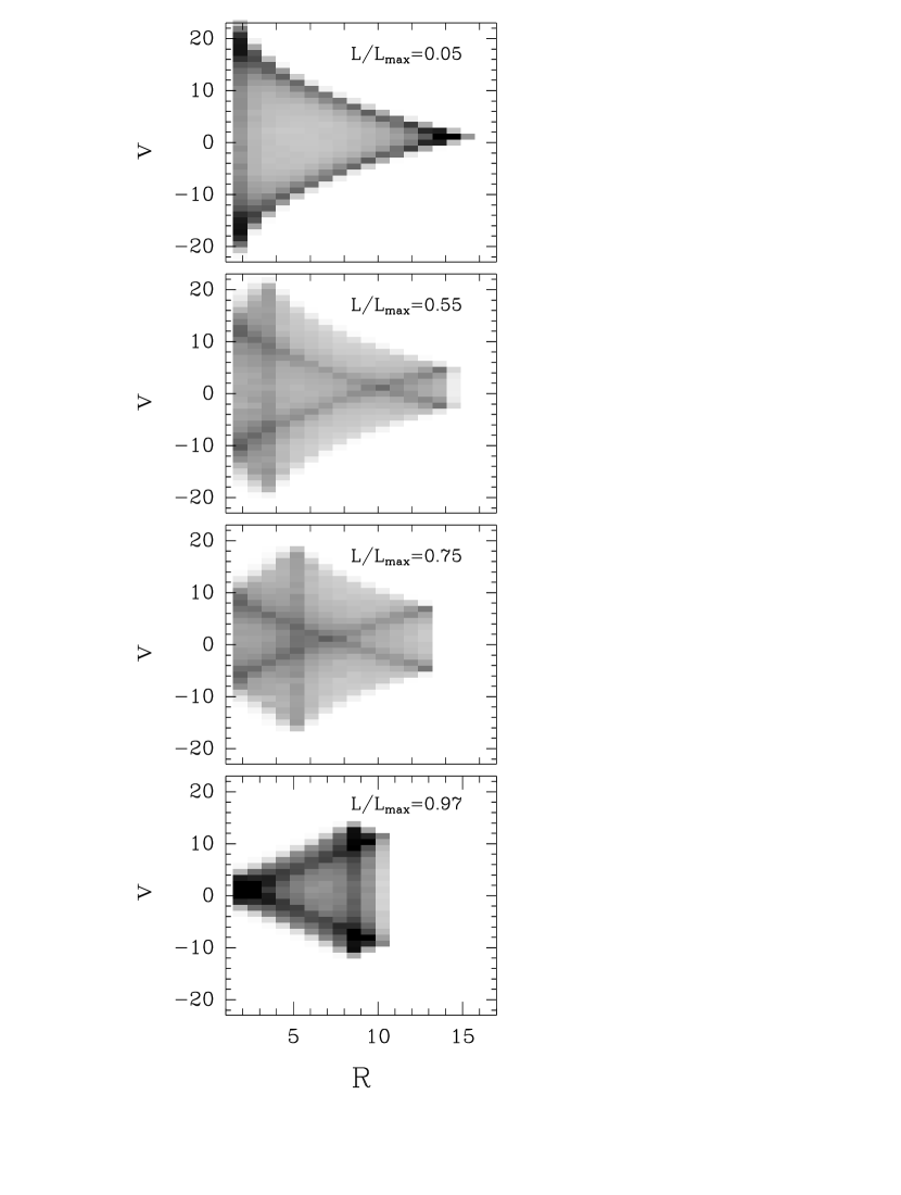
Figure 1:

Figure 2:

Figure 3:

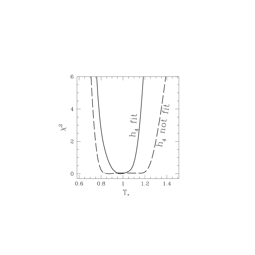
Figure 4:

Figure 5:

Figure 6:

Figure 7:

Figure 8:

Figure 9:

Figure 10:

Figure 11:

References

- (1) Ashman, K.M. 1992, PASP, 104, 1109
- (2) Awaki, H. et al. 1994, PASJ, 46, L65
- (3) Bertin, G., & Stiavelli, M. 1993, Rep. Progr. Phys., 56, 493
- (4) Bertin, G. et al. 1994, A&A, 292, 381
- (5) Binney, J.J., & Mamon, G.A. 1982, MNRAS, 200, 361
- (6) Binney, J.J., & Tremaine, S.D. 1987, Galactic Dynamics (Princeton: Princeton University Press)
- (7) Blumenthal, G., Faber, S., Flores, R., & Primack, J. 1986, ApJ, 301, 27
- (8) Carollo, C.M., & Danziger, I.J. 1994, MNRAS, 270, 523
- (9) Carollo, C.M., de Zeeuw, P.T., van der Marel, R.P., Danziger, I.J., & Qian, E.E. 1995, ApJ, 441, L25 (C95)
- (10) Ciardullo, R., Jacoby, G.H., & Dejonghe, H.B. 1993, ApJ, 414, 454
- (11) Cole, S., & Lacey, C. 1996, MNRAS, 281, 716
- (12) Cretton, N., van der Marel, R.P., Rix, H.-W., & de Zeeuw, P.T. 1997, ApJ, in preparation
- (13) Dejonghe, H.B. 1987, MNRAS, 224, 13.
- (14) Dejonghe, H.B. 1989, ApJ, 343, 113
- (15) Dejonghe, H.B., & Merritt, D. 1992, ApJ, 391, 531
- (16) de Zeeuw, & P.T., Franx, M. 1991, ARA&A 29, 239
- (17) de Zeeuw, P.T. 1995, IAU Symposium 164, Stellar Populations, eds G. Gilmore, P.C. van der Kruit (Dordrecht: Kluwer), 215
- (18) de Zeeuw, P.T. 1996, in Gravitational Dynamics, eds. O. Lahav, E. Terlevich & R. Terlevich (Cambridge: Cambridge Univ. Press), 1
- (19) Forman, C., Jones, C., & Tucker, W. 1985, ApJ, 293, 102
- (20) Franx, M., van Gorkom, J., & de Zeeuw, P.T. 1994, ApJ, 436, 642
- (21) Gerhard, O.E. 1993, MNRAS, 265, 213
- (22) Hernquist, L. 1990, ApJ 356, 359
- (23) Katz, N., & Richstone, D.O., 1985, ApJ, 296, 331
- (24) Kochanek, C. 1994, ApJ, 436, 56
- (25) Kochanek, C. 1995, ApJ, 445, 559
- (26) Kormendy, J., & Richstone, D. 1995, ARA&A, 33, 581
- (27) Kuijken, K. and Merrifield, M. R., 1993, MNRAS, 264, 712
- (28) Lawson, C.L., & Hanson, R.J. 1974, Solving Least Squares Problems (Englewood Cliffs, New Jersey: Prentice–Hall)
- (29) Levison, H.F., & Richstone, D.O. 1985, ApJ, 295, 349
- (30) Maoz, D., & Rix, H.-W. 1993, ApJ, 416, 425
- (31) Merritt, D. 1993, ApJ, 413, 79 (1993a)
- (32) Merritt, D. 1993, in Structure, Dynamics and Chemical Evolution of Elliptical Galaxies, eds. I.J. Danziger, W.W. Zeilinger, & K. Kjär (Münich: ESO), 275 (1993b)
- (33) Merritt, D., & Saha, P. 1993, ApJ, 409, 75 (1993c)
- (34) Merritt, D., & Oh, S.P. 1997, preprint
- (35) Navarro, J., Frenk, C., & White, S.D.M. 1996, ApJ, 462, 563 (NFW)
- (36) Pfenniger, D. 1984, A&A, 141, 171
- (37) Press, W.H., Teukolsky, S.A., Vetterling, W.T., & Flannery, B.P. 1992, Numerical Recipes (Cambridge: Cambridge University Press)
- (38) Richstone, D.O., 1980, ApJ, 238, 103.
- (39) Richstone, D.O., 1984, ApJ, 281, 100.
- (40) Richstone, D.O., & Tremaine, S.D. 1984, ApJ, 286, 27
- (41) Richstone, D.O., & Tremaine, S.D. 1985, ApJ, 296, 370
- (42) Richstone, D.O., & Tremaine, S.D. 1988, ApJ, 327, 82
- (43) Rix, H.-W., 1996a, in Proceedings of the DM 1996 Workshop at Sesto, eds. P. Salucci and M. Sersic.
- (44) Rix, H.-W., 1996b, in The Nature of Elliptical Galaxies, Proceedings of the Second Stromlo Symposium, eds M. Arnaboldi, G. da Costa and P. Saha.
- (45) Rix, H.-W., & White, S.D.M. 1992, MNRAS, 254, 389
- (46) Saglia, R.P., Bertin, G., & Stiavelli, M. 1992, ApJ, 384, 433
- (47) Saglia, R.P. et al. 1993, ApJ, 403, 567
- (48) Saglia, R.P. 1996, in New Light on Galaxy Evolution, Proc. IAU Symp. 171, eds. R. Bender, R.L. Davies (Dordrecht: Kluwer Academic Publishers), 157
- (49) Schwarzschild, M. 1979, ApJ, 232, 236
- (50) Statler, T., Smecker-Hane, T., & Cecil, G. 1996, AJ, 111, 1512
- (51) Tremblay, B., Merritt, D., & Williams, T.B., 1995, ApJ, 443, L5
- (52) van Albada, T.S., Bahcall, J.N., Begeman, K., & Sancisi, R. 1985, ApJ, 295, 305
- (53) van der Marel, R.P. 1991, MNRAS, 253, 710
- (54) van der Marel, R.P., & Franx, M. 1993, ApJ, 407, 525 (vdMF)
- (55) van der Marel, R.P., de Zeeuw, P.T., Rix, H.-W., & Quinlan, G.D. 1997a, Nature, in press
- (56) van der Marel, R.P., de Zeeuw, P.T., Cretton, N. & Rix, H.-W. 1997b, ApJ, in preparation
- (57) Vandervoort, P.O. 1984, ApJ, 287, 475
- (58) Zhao, H.S. 1996, MNRAS, 278, 488