In this lecture I will review some recent progress in improving the accuracy of the calculation of density perturbations resulting from inflation.

1. Introduction

The early universe was very nearly uniform. However, the important caveat in that statement is the word “nearly.” Our current understanding of the origin of structure in the universe is that it originated from small “seed” perturbations, which over time grew to become all of the structure we observe. The best guess for the origin of these perturbations is quantum fluctuations during an inflationary era in the early universe.

The basic idea of inflation is that there was an epoch early in the history of the universe when potential, or vacuum, energy dominated other forms of energy density such as matter or radiation. During the vacuum-dominated era the scale factor grew exponentially (or nearly exponentially) in time. In this phase (known as the de Sitter phase), a small, smooth spatial region of size less than the Hubble radius at that time can grow so large as to easily encompass the comoving volume of the entire presently observable universe.

If the early universe underwent this period of rapid expansion, then one can understand why the universe is approximately smooth on the largest scales, but has structure (people, planets, stars, galaxies, clusters of galaxies, superclusters, etc.). Inflation also predicts that the cosmic background radiation should be very nearly isotropic, with small variations in the temperature. Perhaps all of the structure we see in the universe is a result of quantum-mechanical fluctuations during the inflationary epoch. In this lecture I will explore this possibility.

Because nearly all of the students are familiar with the basics of cosmology, I will not bother to define familiar terms and notation. In general, the notation follows that in The Early Universe (Kolb and Turner, 1990), except that here the scale factor is denoted by $a(t)$.

Since this is a school, I will not provide an exhaustive list of references to original material, but refer to several basic papers (including several review papers) where students can find the references to the original material. The list of references include Bardeen (1980); Stewart (1990); Mukhanov, Feldman, and Brandenberger (1992); Liddle and Lyth (1993); and Lidsey, Liddle, Kolb, Copeland, Barreiro, and Abney (L²KCBA) (1997).

2. Evolution of Perturbations

2.1. Life Beyond the Hubble Radius

An important part of this lecture will be the interplay of physical length scales with the Hubble radius. The time-dependent Hubble radius is defined as the inverse of the expansion rate: $R_{H}(t)\equiv H^{-1}(t)=[8\pi G\rho(t)/3]^{-1/2}$ (the last part of the equation comes from the Friedmann equation for a spatially flat universe). In a radiation-dominated (RD) universe $\rho\propto a^{-4}$ and in a matter-dominated (MD) universe $\rho\propto a^{-3}$, so $R_{H}\propto a^{2}$ in an RD universe and $R_{H}\propto a^{3/2}$ in a MD universe.

First, let us review what is meant by “crossing” the Hubble radius. For the sake of illustration, let’s take a length scale $\lambda$ to be at present $\lambda_{0}=300h^{-1}$Mpc. Today the Hubble radius is $R_{H}(t_{0})=H_{0}^{-1}\sim 3000h^{-1}$Mpc, so $\lambda_{0}/R_{H}(t_{0})=10^{-1}$ and $\lambda_{0}$ is said to be “within” the Hubble radius today. Any physical length scale increases in proportion to the scale factor in an expanding universe. The scale which is $\lambda_{0}$ today, was smaller in the early universe by a factor of $a(t)/a_{0}=1/(1+z)$, where $a_{0}$ is the present scale factor. The Hubble radius also depends upon $a(t)$, e.g., $R_{H}=[a(t)/a_{0}]^{3/2}=1/(1+z)^{3/2}$ in the MD era. So during the MD era the ratio $\lambda(t)/R_{H}(t)$ depends upon redshift as $\lambda(t)/R_{H}(t)=[\lambda_{0}/R_{H}(t_{0})](1+z)^{1/2}=10^{-1}(1+z)^{1/2}$. So for $z\mathrel{\mathchoice{\lower 3.6pt\vbox{\halign{$\mathsurround=0pt\displaystyle\hfill#\hfil$\cr>\crcr\sim\crcr}}}{\lower 3.6pt\vbox{\halign{$\mathsurround=0pt\textstyle\hfill#\hfil$\cr>\crcr\sim\crcr}}}{\lower 3.6pt\vbox{\halign{$\mathsurround=0pt\scriptstyle\hfill#\hfil$\cr>\crcr\sim\crcr}}}{\lower 3.6pt\vbox{\halign{$\mathsurround=0pt\scriptscriptstyle\hfill#\hfil$\cr>\crcr\sim\crcr}}}}100$, the length scale $\lambda$ was outside the Hubble radius, for $z\mathrel{\mathchoice{\lower 3.6pt\vbox{\halign{$\mathsurround=0pt\displaystyle\hfill#\hfil$\cr<\crcr\sim\crcr}}}{\lower 3.6pt\vbox{\halign{$\mathsurround=0pt\textstyle\hfill#\hfil$\cr<\crcr\sim\crcr}}}{\lower 3.6pt\vbox{\halign{$\mathsurround=0pt\scriptstyle\hfill#\hfil$\cr<\crcr\sim\crcr}}}{\lower 3.6pt\vbox{\halign{$\mathsurround=0pt\scriptscriptstyle\hfill#\hfil$\cr<\crcr\sim\crcr}}}}100$, the length scale $\lambda$ was inside the Hubble radius. At $z=100$ we say that a length scale of $300h^{-1}$Mpc crossed the Hubble radius.

Since $\lambda(t)/R_{H}(t)$ decreases in time in a radiation-dominated or matter-dominated universe, any physical length scale $\lambda$ starts larger than $R_{H}$, then crosses the Hubble radius ($\lambda=H^{-1}$) only once. This behavior is illustrated by the left side of Fig. 1.

In order for structure formation to occur via gravitational instability, there must have been small preexisting fluctuations on physical length scales when they crossed the Hubble radius in the RD an MD eras. In the standard big-bang model these small perturbations have to be put in by hand, because it is impossible to produce fluctuations on any length scale while it is larger than $R_{H}$. Since the goal of cosmology is to understand the universe on the basis of physical laws, this appeal to initial conditions is unsatisfactory.

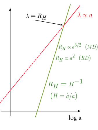
Figure 1: The behavior of the Hubble radius, $R_{H}$, and the physical size, $\lambda$, with the scale factor $a$ during normal expansion (left) and inflationary expansion (right).

That any length scale crosses $R_{H}$ only once is not a fundamental result of anything sacred like Einstein’s equations, the cosmological principle, or special relativity, but it depends upon the assumption of the equation of state. To see how changing the equation of state changes the ratio $\lambda(t)/R_{H}(t)$, let’s define $L(t)$ to be the dimensionless ratio $\lambda(t)/R_{H}(t)$. Obviously, if $L(t)$ is smaller than unity, the scale is within the Hubble radius and it is possible to imagine some microphysical process establishing perturbations on that scale, while if $L(t)$ is larger than unity, it is beyond the Hubble radius and no microphysical process can account for perturbations on that scale. Now $R_{H}(t)=H^{-1}(t)=a(t)/\dot{a}(t)$ and $\lambda(t)\propto a(t)$, so $L(t)$ is proportional to $\dot{a}(t)$, and $\dot{L}(t)$ scales as $\ddot{a}(t)$, which from the Einstein equation is proportional to $-(\rho+3p)$. There are two possible scenarios for $\dot{L}(t)$ depending upon the sign of $\rho+3p$:

$$\dot{L}(t)\left\{\begin{array}[]{lll}<0\rightarrow&R_{H}(t)\mbox{ grows faster than }\lambda(t),&\mbox{occurs for }\rho+3p>0\\ >0\rightarrow&R_{H}(t)\mbox{ grows more slowly than }\lambda(t),&\mbox{occurs for }\rho+3p<0.\end{array}\right.$$ (1)

If during some epoch the equation of state was such that $\rho+3p<0$, then scales larger than $R_{H}$ remained larger than $R_{H}$, while scales smaller than the Hubble radius were destined eventually to grow larger than the Hubble radius. The opposite behavior obtains during the standard RD and MD epochs when $\rho+3p>0$. During these epochs scales smaller than $R_{H}$ remain smaller than $R_{H}$ and scales larger than $R_{H}$ eventually become smaller than $R_{H}$.

Now if $\rho+3p<0$ in the early universe and $\rho+3p>0$ in the later universe, then it is possible to have a “double-cross” situation illustrated on the right side of Fig. 1. In the double-cross scenario, length scales start smaller than the Hubble radius during the phase when $\rho+3p<0$ (the inflationary phase), cross the Hubble radius, then remain larger than the Hubble radius. During the standard phase, scales of astrophysical interest start larger than the Hubble radius, cross the Hubble radius, then remain smaller than the Hubble radius.

Unlike the standard model, the double-cross model has the feature that it is possible to imprint perturbations on a scale as it crosses the Hubble radius during the inflationary phase, so one can imagine a reason to have preexisting perturbations on scales recrossing the Hubble radius during the RD-MD epochs.

2.2. Metric Perturbations on Scales Larger than $R_{H}$

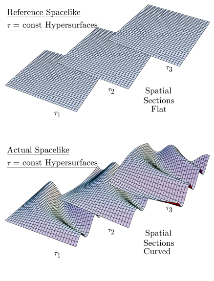
Figure 2: In the reference unperturbed universe, constant-time surfaces have constant spatial curvature (zero for a flat FRW model). In the actual perturbed universe, constant-time surfaces have spatially varying spatial curvature.

What we are interested in following the evolution of a spacetime which is neither homogeneous nor isotropic. We will do this by following the evolution of the differences between the actual spacetime and a well understood reference spacetime. So we will consider small perturbations away from the homogeneous, isotropic spacetime (see Fig. 2).

When one studies “perturbations” it is necessary to specify a reference background system. The reference system in our case is the spatially flat Friedmann–Robertson–Walker (FRW) spacetime, with line element $ds^{2}=a^{2}(\tau)\left\{d\tau^{2}-\delta_{ij}dx^{i}dx^{j}\right\}$, where $\tau$ is conformal time, related to “normal” time by $a^{2}d\tau^{2}=dt^{2}$. Sometimes equations will be written in terms of conformal time $\tau$, and sometimes in terms of coordinate time $t$. Derivatives with respect to conformal time will be denoted by a prime, while usual time derivatives are denoted by a dot, e.g., the Hubble parameter can be defined as $H(t)\equiv\dot{a}/a$, or ${\cal H}(\tau)=a^{\prime}/a=Ha$.

The most general form of a metric describing small perturbations away from the flat FRW metric contains scalar, vector, and tensor perturbations [the covariant decomposition of $\delta g_{\mu\nu}$ is given in Stewart (1990)]. For the moment, we will only be interested in the scalar perturbations. The perturbed line element including the scalar perturbations can be written in terms of four scalar functions $\{A,\ B,\ \psi,\ E\}$:

$$ds^{2}=a^{2}(\tau)\left\{(1+2A)d\tau^{2}-2\partial_{i}B\,dx^{i}d\tau-\left[(1-2\psi)\delta_{ij}+2\partial_{i}\partial_{j}E\right]dx^{i}dx^{j}\right\}.$$ (2)

Now because of the residual gauge freedom, not all of the four scalar perturbation functions $\{A,\ B,\ \psi,\ E\}$ are independent. For instance if one works in the synchronous gauge, all hypersurfaces have the same time. In this gauge $A=B=0$, and the line element is $ds^{2}=a^{2}(\tau)\left\{d\tau^{2}-\left[(1-2\psi)\delta_{ij}+2\partial_{i}\partial_{j}E\right]dx^{i}dx^{j}\right\}$. In the longitudinal gauge $B=E=0$, and the line element is $ds^{2}=a^{2}(\tau)\left\{(1+2A)d\tau^{2}-\left[(1-2\psi)\delta_{ij}\right]dx^{i}dx^{j}\right\}$.

It is sometimes bewildering to read the literature because everyone seem to have his/her favorite gauge. But really smart people support freedom of choice, and work with combinations of the gauge-invariant scalar functions $\Psi$ and $\Phi$ first found by Bardeen (1980):

$$\Psi = \psi-{\cal H}(B-E^{\prime})$$ (3)

$$\Phi = A+a^{-1}[(B-E^{\prime})a]\,^{\prime}.$$ (4)

Note that in the longitudinal gauge $\Phi=A$ and $\Psi=\psi$.

2.3. Perturbations in the Stress-Energy Tensor

Inflation assumes that the universe was dominated by something with an equation of state that satisfies the inequality $\rho+3p<0$. Such a component of the energy density is usually called “vacuum energy.” Since today we know that the vacuum energy must be very small (compared to what is required for inflation), any inflationary model has to have some dynamics for changing the vacuum energy. It is convenient to imagine that the dynamics of the change in the equation of state during inflation is described by the usual dynamics of a minimally coupled scalar field evolving under the influence of a scalar potential. This mysterious scalar field, denoted by $\phi$, is known as the inflaton, and its potential, $V(\phi)$, is known as the inflaton potential.

One assumes that the inflaton field is homogeneous in the reference spacetime, $\phi({\bf x},\tau)=\phi_{0}(\tau)$, and satisfies the equation of motion $\ddot{\phi}_{0}+3H\dot{\phi}_{0}+{{V,_{\phi}}}=0$. (Since “prime” was used to denote $d/d\tau$, I will use $X,_{\phi}$ to denote $dX/d\phi$.) This field equation, together with the Friedmann equation, can be solved to find the evolution of the background spacetime and scalar field. Alternatively, one can view the scalar field itself as the dynamical variable of the system. This allows the Einstein–scalar-field equations to be written as a set of first-order, non-linear differential equations (Grishchuk & Sidorav 1988; Muslimov 1990; Salopek & Bond 1990, 1991; Lidsey 1991a)

$$[{{H,_{\phi}}}(\phi)]^{2}-\frac{12\pi}{m_{Pl}^{2}}H^{2}(\phi) = -\frac{32\pi^{2}}{m_{P}l^{4}}V(\phi)$$ (5)

$$\dot{\phi} = -\frac{m_{Pl}^{2}}{4\pi}{{H,_{\phi}}}.$$ (6)

In the actual perturbed spacetime there are small perturbations about the background value: $\phi({\bf x},\tau)=\phi_{0}(\tau)+\delta\phi({\bf x},\tau)$. Of course we will be interested in the evolution of $\delta\phi$.

Now just as the metric perturbations are gauge dependent, the scalar field fluctuations are also. But one can circumvent the usual problems associated with gauge freedom by constructing a suitable gauge-invariant scalar field fluctuation, $\widetilde{\delta\phi}=\delta\phi+\phi_{0}^{\prime}(B-E^{\prime})$.

2.4. Perturbation Spectra

Of great convenience is the particular gauge-invariant quantity

$${{\cal R}}=\Psi-\frac{{\cal H}}{\phi_{0}^{\prime}}\widetilde{\delta\phi}=\psi-\frac{H}{\dot{\phi}}\delta\phi.$$ (7)

Clearly ${{\cal R}}$ defined by the first equality of Eq. (7) is gauge invariant because it is constructed explicitly from gauge-invariant terms. However even the second form in Eq. (7) is gauge invariant, as when one performs a gauge transformation the non-gauge-invariant terms in $\psi$ cancels the non-gauge-invariant terms in the $\delta\phi$ term.

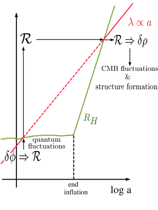
Figure 3: Quantum fluctuations in the inflaton field during inflation lead to fluctuations in the gauge-invariant quantity ${{\cal R}}$. As a particular length scale passes outside of the Hubble radius, the fluctuations are “frozen in” because ${{\cal R}}$ is constant outside the Hubble radius. When the length scale reenters the Hubble radius in the RD or MD era, fluctuations in ${{\cal R}}$ appear as energy density fluctuations.

${{\cal R}}$ has a simple physical interpretation in the synchronous gauge, where $\nabla^{2}{{\cal R}}={{}^{3}\!R}/4$ with ${}^{3}\!R$ the three-dimensional Ricci curvature on the spatial hypersurface. Now the usefulness of ${{\cal R}}$ follows from the fact that as shown by Bardeen (1980), ${{\cal R}}$ is constant on scales much larger than $R_{H}$.

The picture of the generation of quantum fluctuations during inflation can be appreciated by studying Fig. 3.

Now ${{\cal R}}$ is related to the observationally determined power spectrum. The first step in developing the relation is to expand ${{\cal R}}$ in terms of Fourier modes ${{\cal R}}_{k}$

$${{\cal R}}({\bf x})=\int\frac{d^{3}\!k}{(2\pi)^{3/2}}{{\cal R}}_{k}(\tau)\ e^{i{\bf k}\cdot{\bf x}}.$$ (8)

Now following the usual procedure, if we form $\langle{\cal R}({\bf x}){\cal R}({\bf x})\rangle^{1/2}$, where $\langle\cdots\rangle$ indicates the spatial average, we find that it is proportional to $\int k^{2}|{\cal R}_{k}|^{2}dk/k$, so $k^{3/2}|{\cal R}_{k}|$ is the power in ${\cal R}$ per decade of $k$. If the curvature perturbation is independent of $k$, then the “power-per-decade” is constant, and $|{\cal R}_{k}|\propto k^{-3/2}$. Putting in the factors of $2\pi$, we define the scalar spectrum $A_{S}(k)$ by

$$\frac{k^{3}}{2\pi^{2}}\ \langle{{\cal R}}_{k}{{\cal R}}_{l}^{*}\rangle=\frac{25}{4}\ A_{S}^{2}(k)\ \delta^{3}({\bf k}-{\bf l}),$$ (9)

where $A_{S}(k)$ is the primordial scalar density perturbation power spectrum. If ${\cal R}$ is independent of scale outside of the Hubble radius, then $A_{S}(k)$ will be independent of $k$. The primordial power spectrum, $A_{S}(k)$, is related to $P_{S}(k)$, the power spectrum observed in large-scale structure (LSS) surveys and cosmic background radiation (CBR) experiments.

To find the relation between $A_{S}(k)$ and $P_{S}(k)$, it is important to appreciate that $A_{S}(k)$ is the amplitude when a scale $k$ crosses the Hubble radius, i.e., when $k=aH$. Now if we specify the perturbation spectrum on a particular space-like hypersurface, rather than as each scale crosses the Hubble radius, we have to realize that we are specifying a gauge-dependent quantity beyond the Hubble radius. We will denote the perturbation defined this way as $(\delta\rho/\rho)_{k}$. In the synchronous gauge and in the comoving gauge, the density perturbation of wavenumber $k$ grows as $(\delta\rho/\rho)_{k}\propto(aH)^{-2}$ for $k<aH$ in both the MD and RD eras. So for scales well outside the Hubble radius, $(\delta\rho/\rho)_{k}\propto[k^{2}/(aH)^{2}]A_{S}(k)$, so that when $aH=k$, $(\delta\rho/\rho)_{k}=A_{S}(k)$.

For scales inside the Hubble radius the synchronous gauge and the comoving gauge coincide, and $(\delta\rho/\rho)_{k}$ is approximately constant in the RD era and grows as $(\delta\rho/\rho)_{k}\propto(aH)^{-2}$ in the MD era. So just around the time of matter domination, on scales smaller than $R_{H}$ (i.e., $k\gg(aH)_{EQ}$), $(\delta\rho/\rho)_{k}$ has the approximate value it had when it crossed the Hubble radius, so $(\delta\rho/\rho)_{k}\sim A_{S}(k)$ for $k\gg(aH)_{EQ}$. After matter domination $(\delta\rho/\rho)_{k}$ grows as $(aH)^{-2}\sim a\propto t^{2/3}$ on all scales, so $(\delta\rho/\rho)_{k}$ will continue to have the shape it did just after matter domination (at least in the regime of linear evolution).

The transition between scales larger than $R_{H}$ at $t_{EQ}$ and scales smaller than $R_{H}$ at $t_{EQ}$ can be encoded in a “transfer function” $T(k)$, by writing $(\delta\rho/\rho)_{k}=(k/aH)^{2}T(k)A_{S}(k)$ (see e.g., Liddle and Lyth, 1993). In order to reproduce the behavior discussed above, the function $T(k)$ must have the limiting forms $T(k)\rightarrow 1$ for $k\ll aH$ and $T(k)\rightarrow k^{-2}$ for $k\gg aH$.

Now the power spectrum $P_{S}(k)$ is defined by $(\delta\rho/\rho)_{k}^{2}\propto k^{3}P_{S}(k)$, so in terms of the primordial spectrum $A_{S}(k)$ and the transfer function $T(k)$, $P_{S}(k)$ is given by $P_{S}(k)\propto kT^{2}(k)A_{S}^{2}(k)$. Note that if the primordial spectrum is independent of scale, i.e., if $A_{S}^{2}(k)$ is independent of $k$—the Harrison-Zel’dovich spectrum, then $P_{S}(k)\propto k$ for $k\ll(aH)_{EQ}$ and $P_{S}(k)\propto k^{-3}$ for $k\gg(aH)_{EQ}$. If we write $A_{S}(k)$ as a power law, $A_{S}^{2}(k)=A_{S}^{2}(k_{0})(k/k_{0})^{n-1}$, then $P_{S}$ will be a power law also: $P_{S}(k)\propto k^{n}$, with $n=1$ corresponding to the value for constant amplitude perturbations at Hubble radius crossing.

Finally, we must understand the relation between wavenumber $k$ and field value $\phi$. During the evolution of the scalar field the background value of $\phi$ changes in time. Now associated with a particular value of $\phi$ is a length scale with comoving wavenumber $k$ crossing the Hubble radius at the time the scalar field value is $\phi$. The easiest relation to find is the differential form found from the expression $k=aH$:

$$\frac{d\ln k}{d\phi}=\frac{{{H,_{\phi}}}}{H}+\frac{{{a,_{\phi}}}}{a}=\frac{{{H,_{\phi}}}}{H}-\frac{4\pi}{m_{Pl}^{2}}\frac{H}{{{H,_{\phi}}}},$$ (10)

where the last equality follows from Eq. (5).

3. Scalar Perturbations from Inflation

3.1. Textbook Treatment

In the standard textbook treatment one expands fluctuations of the inflaton field in a Fourier expansion

$$\langle\delta\phi^{2}\rangle^{1/2}=\int\frac{dk}{k}\,k^{3}\left|\delta_{k}\right|^{2}.$$ (11)

Then one identifies $(\delta\phi)_{k}\equiv k^{3/2}|\delta\phi_{k}|$ as the fluctuation in the inflaton on the length scale $2\pi/k$. One knows that a scalar field has quantum fluctuations in deSitter space, or more precisely, the quantum fluctuations of a scalar field in deSitter space differ from the quantum fluctuations of a scalar field in flat space. The quantum fluctuations of a field in deSitter space at Hubble radius crossing (i.e., on scales $k=aH$, where $k$ is the comoving wavenumber) result in $(\delta\phi)_{k=aH}=H/2\pi$.

Now in the $\psi=0$ gauge, using the above result for the scalar field fluctuation gives ${{\cal R}}=(H/\dot{\phi}_{0})(\delta\phi)_{k=aH}\sim H^{2}/\dot{\phi}_{0}$. Now we can express $H^{2}$ and $\dot{\phi}_{0}$ in terms of the inflaton potential and its derivative. The background equation of motion from Section 2.3 in the slow-roll limit (ignoring the $\ddot{\phi}$ term) gives $\dot{\phi}\sim{{V,_{\phi}}}/3H$, and the Friedmann equation relates $H$ and $V(\phi)$: $H^{2}=8\pi\rho/3m_{Pl}^{2}\sim V(\phi)/m_{Pl}^{2}$. Substituting $V$ and ${{V,_{\phi}}}$ gives the familiar result for the perturbation spectrum first found in this manner by Bardeen, Steinhart, and Turner (1983),

$$k^{3/2}{{\cal R}}_{k}\sim A_{S}(k)\sim\frac{1}{m_{Pl}^{3}}\frac{V^{3/2}(\phi)}{{{V,_{\phi}}}}.$$ (12)

Since the scale factor increases so rapidly during inflation, all astrophysical scales of interest correspond to a rather narrow range of inflaton field values. For flat potentials, $V(\phi)$ and ${{V,_{\phi}}}(\phi)$ does not change much during inflation, so one expects $A_{S}(k)$ to be roughly independent of $k$. This is the reason for the often repeated “result” that inflation leads to an approximate Harrison-Zel’dovich spectrum of scalar density perturbations.

3.2. The Three Step Program for Better Predictions

The calculation of $A_{S}(k)$ in Eq. (12) was sufficiently accurate for a decade. But even with present-day data, and especially looking forward to the wealth of information expected in the near future, such as the angular power spectrum of CMB fluctuations up to multipole number of more than $10^{3}$, more accurate predictions are required.

As the result of considerable effort, in the past few years some progress has been made in improving the accuracy of the calculation of the density perturbation spectrum. Let me describe three basic steps in the road toward better accuracy:

1. a better treatment of the background classical dynamics by use of Hamilton-Jacobi formalism,

2. a better formalism of quantum corrections by use of the variational approach, and

3. the calculation of the spectra in terms of slow-roll parameters.

I have already discussed the advantage of treating $H$ as fundamental, and parameterizing its evolution by $\phi$ rather than time. In principle, the Hamilton–Jacobi formalism enables one to treat the dynamical evolution of the scalar field exactly, at least at the classical level. In practice, however, the separated Hamilton-Jacobi equation, the first line of Eq. (5), is rather difficult to solve. On the other hand, the analysis can proceed straightforwardly once the functional form of the expansion parameter $H(\phi)$ has been determined. This suggests that one should view $H(\phi)$ as the fundamental quantity in the analysis (Lidsey 1991b, 1993). This is in contrast to the more traditional approaches to inflationary cosmology, whereby the particle physics sector of the model — as defined by the specific form of the inflaton potential $V(\phi)$ — is regarded as the input parameter.

It proves convenient to express the scalar and tensor perturbation spectra in terms of $H(\phi)$ and its derivatives. The slow-roll approximation is an expansion in terms of quantities derived from appropriate derivatives of the Hubble expansion parameter. Since at a given point each derivative is independent, there are in general an infinite number of these terms, but only the first few enter into any expressions of interest. The first three are defined as

$$\epsilon(\phi)\equiv\frac{3\dot{\phi}^{2}}{2}\left[V+\frac{1}{2}\dot{\phi}^{2}\right]^{-1}=\frac{m_{{\rm Pl}}^{2}}{4\pi}\left(\frac{{{H,_{\phi}}}(\phi)}{H(\phi)}\right)^{2}\,,$$ (13)

$$\eta(\phi)\equiv-\frac{\ddot{\phi}}{H\dot{\phi}}=\frac{m_{{\rm Pl}}^{2}}{4\pi}\frac{{{H,_{\phi\phi}}}(\phi)}{H(\phi)}=\epsilon-\frac{m_{{\rm Pl}}\,{{\epsilon,_{\phi}}}}{\sqrt{16\pi\epsilon}}\,,$$ (14)

$$\xi(\phi)\equiv\frac{m_{{\rm Pl}}^{2}}{4\pi}\left(\frac{{{H,_{\phi}}}(\phi){{H,_{\phi\phi\phi}}}(\phi)}{H^{2}(\phi)}\right)^{1/2}=\left[\epsilon\eta-\left(\frac{m_{{\rm Pl}}^{2}\,\epsilon}{4\pi}\right)^{1/2}{{\eta,_{\phi}}}\right]^{1/2}\,.$$ (15)

One need not be concerned as to the sign of the square root in the definition of $\xi$; it turns out that only $\xi^{2}$, and not $\xi$ itself, will appear in our formulae. We emphasize that the choice $\dot{\phi}>0$ implies that $\sqrt{\epsilon}=-\sqrt{m_{{\rm Pl}}^{2}/4\pi}\,{{H,_{\phi}}}/H$.

One can show that inflation ends when $\epsilon=1$. The slow-roll approximation, as I use it here, involves assuming $\{\epsilon,\ \eta,\ \xi\}$ are all less than unity. This is somewhat more restrictive than just saying that $H$ changes slowly enough for inflation to occur: that only requires $\epsilon<1$.

Probably the most important advance is the development of the Mukhanov formalism for the perturbation calculation. Recall that the action for the Einstein–scalar field system is

$$S=-\int d^{4}\!x\sqrt{-g}\left[\frac{m_{Pl}^{2}}{16\pi}R-\frac{1}{2}(\nabla\phi)^{2}+V(\phi)\right],$$ (16)

with $g_{\mu\nu}=g_{\mu\nu}^{FRW}+\delta g_{\mu\nu}(A,B,\psi,E)$ and $\phi=\phi_{0}(\tau)+\delta\phi({\bf x},\tau)$.

Before quantizing the system, one must express the theory in terms of the ADM variables, expand to second order in the perturbations, apply the background field equations, and integrate by parts when judicious. Now the procedure is quite long and tedious. Details can be found in the review article of Mukhanov, Feldman, and Brandenberger (1992). When the dust settles, the variation of the action can be expressed in terms of the dynamical variable $u=a(\delta\phi+\phi_{0}^{\prime}\psi/{\cal H})=z{\cal R}$, where $z=a\phi_{o}^{\prime}/{\cal H}=a\dot{\phi}_{0}/H$:

$$\delta_{2}S=\frac{1}{2}\int d^{4}\!x\left(u^{\prime 2}-\delta^{ij}u,_{i}u,_{j}+\frac{z^{\prime\prime}}{z}u^{2}\right).$$ (17)

Now this is really remarkable, because the complicated dynamics of scalar field perturbations coupled to metric perturbations can be cast into the dynamics of a system we know well: a scalar field $u$ in flat spacetime with (time-dependent and negative) mass $m^{2}=-z^{\prime\prime}/z$.

Now scalar field theory in flat space is well understood. So we can use the tool of scalar quantum field theory as a sort of hammer to pound out the answer. Of course, we have to make sure we have the right tool, because as the saying goes, “when you have a hammer in your hand, everything you see looks like a nail.”

3.3. Quantization

The quantization of the action in Eq. (17) is really rather straightforward: From the scalar field $u({\bf x},\tau)$, form the conjugate momentum $\pi({\bf x},\tau)$, and form the Hamiltonian from $u({\bf x},\tau)$ and $\pi({\bf x},\tau)$. Then promote the classical field and its conjugate momentum to operators, $u({\bf x},\tau)\rightarrow\widehat{u}({\bf x},\tau)$, and $\pi({\bf x},\tau)\rightarrow\widehat{\pi}({\bf x},\tau)$ and impose the canonical equal-time commutation relations $[\widehat{u}({\bf x},\tau),\widehat{u}({\bf y},\tau)]=[\widehat{\pi}({\bf x},\tau),\widehat{\pi}({\bf y},\tau)]=0$, and $[\widehat{u}({\bf x},\tau),\widehat{\pi}({\bf y},\tau)]=i\delta^{3}({\bf x}-{\bf y})$.

If one expands the field operator in Fourier modes associated with creation and annihilation operators $\widehat{a}_{k}^{\dagger}$ and $\widehat{a}_{k}$, then the field becomes

$$\widehat{u}({\bf x},\tau)=(2\pi)^{-3/2}\int d^{3}\!k\left[u_{k}(\tau)\widehat{a}_{k}e^{i{\bf k}\cdot{\bf x}}+u_{k}^{*}(\tau)\widehat{a}^{\dagger}_{k}e^{-i{\bf k}\cdot{\bf x}}\right].$$ (18)

The field equation for $u_{k}$ is the familiar Klein–Gordan equation

$$u_{k}^{\prime\prime}+\left(k^{2}-\frac{z^{\prime\prime}}{z}\right)u_{k}=0.$$ (19)

Of course we must specify the boundary condition. In our case, we want $u_{k\gg aH}\rightarrow e^{-ik\tau}/k^{1/2}$, i.e., plane-wave solutions.

It is pleasing to note that any solution to Eq. (19) will have the feature that well beyond the Hubble radius, ${\cal R}_{k}$ will be constant. Note that in the limit $k\rightarrow 0$ the field equation becomes $u_{k}^{\prime\prime}-(z^{\prime\prime}/z)u_{k}=0$, which obviously has solution $u_{k}\propto z$. Now since ${\cal R}_{k}=u_{k}/z$, on scales much larger than the Hubble radius ${\cal R}_{k}\rightarrow$ constant.

4. Tensor Perturbations

In addition to the scalar perturbations in Eq. (2), the most general metric contains perturbations that transform like a tensor on the spatial hypersurfaces. These tensor perturbations enter the metric as

$$ds^{2}=a^{2}(\tau)\left[d\tau^{2}-(\delta_{ij}+{h_{ij}})dx^{i}dx^{j}\right].$$ (20)

As can be seen by explicit calculation from the Einstein equations, the metric perturbation ${h_{ij}}$ does not couple to the stress-energy tensor, but describes the propagation of gravitational waves. The gravitational waves are not important for large-scale structure, but they do have an effect of the CMB, at least for small multipole number.

Since by construction ${h_{ij}}$ is a transverse, traceless tensor, it has two degrees of freedom, usually denoted as $h_{\times}$ and $h_{+}$. (From the quantum view, gravitational waves are the propagating part of the gravitational degrees of freedom, corresponding to a massless spin-two particle, which of course has two degrees of freedom.)

Now just as was done for the scalar degrees of freedom, one substitutes the metric Eq. (20) into the Einstein–Hilbert action, and expands to quadratic order in ${h_{ij}}$, with the result

$$\delta_{2}S=\frac{m^{2}_{Pl}}{64\pi}\int d\tau d^{3}\!x\,a^{2}(\tau)\,\partial_{\mu}h^{i}_{~{}j}\partial^{\mu}h_{i}^{~{}j}.$$ (21)

Since our goal is quantization, and we know how to quantize scalar field theory, we want to make $\delta_{2}S$ look as much as possible like the action for a scalar field. To this end, it is very convenient to define the rescaled variable $P^{i}_{~{}j}(x)=(m^{2}_{Pl}/32\pi)^{1/2}a(\tau)h^{i}_{~{}j}(x)$. In terms of $P^{i}_{~{}j}(x)$, $\delta_{2}S$ becomes

$$\delta_{2}S=\frac{1}{2}\int d\tau\,d^{3}\!x\,\left[\left(\partial_{\tau}P_{i}^{~{}j}\right)\left(\partial_{\tau}P^{i}_{~{}j}\right)-\delta^{mn}\left(\partial_{m}P_{i}^{~{}j}\right)\left(\partial_{n}P^{i}_{~{}j}\right)+\frac{a^{\prime\prime}}{a}P_{i}^{~{}j}P^{i}_{~{}j}\right].$$ (22)

This may be interpreted as the action for two scalar fields in Minkowski spacetime, each with effective mass squared $-a_{\tau\tau}/a$. We can now proceed with quantization exactly as in the scalar case.

Again, just as in the scalar case for ${\cal R}$, we perform a Fourier decomposition of $P^{i}_{~{}j}$. But since there are two degrees of freedom, we must include a polarization tensor ${\epsilon^{i}}_{j}({\bf k};\lambda)$, which satisfies the conditions $\epsilon_{ij}=\epsilon_{ji}$, $\epsilon_{ii}=0$, $k^{i}\epsilon_{ij}=0$ and ${\epsilon^{i}}_{j}({\bf k},\lambda){\epsilon_{i}}^{j*}({\bf k},\lambda^{\prime})=\delta_{\lambda\lambda^{\prime}}$. The analysis is further simplified if we choose $\epsilon_{ij}(-{\bf k},\lambda)=\epsilon_{ij}^{*}({\bf k},\lambda)$. The Fourier decomposition can be written as

$$P^{i}_{~{}j}=\sum_{\lambda=\times,+}\int\frac{d^{3}\!k}{(2\pi)^{3/2}}\ \ v_{k,\lambda}\ \epsilon^{i}_{~{}j}(k;\lambda)\ e^{i{\bf k}\cdot{\bf x}}.$$ (23)

In terms of $v_{k}$, the spectrum of gravitational waves, $A_{T}(k)$, is defined as

$$\frac{k^{3}}{2\pi^{2}}\langle{v}_{{\bf k},\lambda}{v}^{*}_{{\bf l},\lambda}\rangle=\frac{10^{2}m_{{\rm Pl}}^{2}a^{2}}{32\pi}\,A_{T}^{2}(k)\,\delta^{(3)}({\bf k}-{\bf l})\,.$$ (24)

Now returning to the quantization of the perturbations, in momentum space the tensor perturbation action is

$$\delta_{2}S=\frac{1}{2}\sum_{\lambda=+,\times}\int d\tau d^{3}\!k\left[\left(\partial_{\tau}\left|v_{k,\lambda}\right|\right)^{2}-\left(k^{2}-\frac{a^{\prime\prime}}{a}\right)\left|v_{k,\lambda}\right|^{2}\right]\,.$$ (25)

We can now quantize $v_{k,\lambda}$ in the usual way, promoting the field to an operator with canonical quantization conditions.

The mode equation for $v_{k}$ becomes

$$\frac{d^{2}v_{k}}{d\tau^{2}}+\left(k^{2}-\frac{a^{\prime\prime}}{a}\right)v_{k}=0\,.$$ (26)

This equation can be compared to the mode equation for scalar perturbations, Eq. (19). The mode equation is somewhat simpler than the scalar case because $a^{\prime\prime}/a=2a^{2}H^{2}(1-\epsilon/2)$ is generally a simpler function than $z^{\prime\prime}/z$.

5. A Variety of Models (Some Realistic, Others Illustrative)

5.1. Solution Procedure

The procedure is simple (in principle): solve Eq. (19) for $u_{k}$, then find ${\cal R}_{k}=u_{k}/z$ to give $A_{S}(k)$, which together with a transfer function, yields the power spectrum which can be compared to observations. Then solve Eq. (26) for $v_{k}$, to give $A_{T}(k)$.

The trouble is that exact solutions to the wave equations are hard to find, partly because the mass terms are so complicated:

$$\frac{z^{\prime\prime}}{z} = 2a^{2}H^{2}\left[1+\epsilon-\frac{3}{2}\eta+\epsilon^{2}-2\epsilon\eta+\frac{1}{2}\eta^{2}+\frac{1}{2}\xi^{2}\right],$$ (27)

$$\frac{a^{\prime\prime}}{a} = 2a^{2}H^{2}\left(1-\frac{1}{2}\epsilon\right)$$ (28)

where the $\tau$ dependence of $H,\ \epsilon,\ \eta,$ and $\xi$ are found from their dependence upon $\phi$. In fact, only two exact solutions of Eqs. (19) and (26) are known. The first is a power-law solution found by Stewart and Lyth (1993), and the second, yet unnamed, has been found by Easther (1996).

The first step is to express the conformal time, $d\tau=dt/a(t)$ in terms of $aH$ and the slow-roll parameters. In general the result is

$$\tau=\int\frac{da}{a^{2}H}=-\frac{1}{aH}+\int\frac{\epsilon}{a^{2}H}\ da.$$ (29)

If $\epsilon$ is constant, then $\tau^{-1}=-aH(1-\epsilon)$ ($\tau$ is negative during inflation, with $\tau=0$ corresponding to the infinite future). If $\epsilon$ is not constant, then integrating by parts an infinite number of times, one can obtain

$$\tau=-\frac{1}{aH}\frac{1}{1-\epsilon}-\frac{2\epsilon\zeta}{aH}+\mbox{expansion in slow-roll parameters $\zeta$ etc.}\,,$$ (30)

where $\zeta=\epsilon-\eta$, and $\epsilon$ can now have arbitrary time dependence.

In the next section I will review the exact power-law solution, and and the section after that I will discuss how to use that exact solution to construct perturbative solutions for other models.

5.2. Power-Law Inflation

In the power-law model the Hubble parameter is expressed in terms of the Planck mass and a parameter $p$: $H(\phi)\propto\exp\sqrt{4\pi\phi^{2}/pm_{Pl}^{2}}$, which results from a scalar potential of the form $V(\phi)\propto e^{\phi}$ (Abbott and Wise 1984, Lucchin and Matarrese 1985). Obviously this type of potential is not a fundamental, renormalizable scalar potential, but it is the type of effective low-energy potential for dilaton-like degrees of freedom in string theories and Kaluza-Klein theories.

For $H(\phi)\propto e^{\phi}$, $\epsilon$, $\eta$, and $\xi$ will be equal and constant: $\epsilon=\eta=\xi=p^{-1}$.

Now one can proceed to find $z^{\prime\prime}/z$ and $a^{\prime\prime}/a$, with the result $z^{\prime\prime}/z=(\nu^{2}-1/4)/\tau^{2}$ and $a^{\prime\prime}/a=(\mu^{2}-1/4)/\tau^{2}$, where $\nu=(3/2)+(p-1)^{-1}$ and $\mu=(3/2)+(p-1)^{-1}$ (For power-law inflation $\nu$ and $\mu$ coincide, though in general they do not.)

For power-law inflation the mode equations are simply a Bessel equation:

$$\left[\frac{d^{2}}{d\tau^{2}}+k^{2}-\frac{\nu^{2}-4^{-1}}{\tau^{2}}\right]u_{k} = 0$$ (31)

$$\left[\frac{d^{2}}{d\tau^{2}}+k^{2}-\frac{\mu^{2}-4^{-1}}{\tau^{2}}\right]v_{k} = 0,$$ (32)

which for the boundary conditions we impose are solved by $H_{\nu}^{(1)}(-k\tau)$ and $H_{\mu}^{(1)}(-k\tau)$, Hankel functions of the first kind of order $\nu$ and $\mu$.

We are interested in the asymptotic forms of $u_{k}/z$ and $v_{k}$ for $k\ll aH$, which are easily found to be

$$u_{k} \rightarrow e^{i(\nu-1/2)\pi/2}2^{\nu-3/2}\frac{\Gamma(\nu)}{\Gamma(3/2)}\frac{1}{\sqrt{2k}}(-k\tau)^{-\nu+1/2}$$ (33)

$$v_{k} \rightarrow {\mbox{above with}}\ \nu\rightarrow\mu$$ (34)

which yields $A_{S}(k)\propto H^{2}/|H^{\prime}|$ and $A_{T}(k)\propto H$, with both expressions evaluated at $k=aH$. Now using the fact that at Hubble radius crossing $H(\phi)\propto k^{1/p}$ from Eq. (10), we find a power-law spectrum $A_{S}(k)$ and $A_{T}(k)$ proportional to $k^{-1/p}$.

The scalar spectral index is defined as $n(k)-1=d\ln A_{S}^{2}/d\ln k$. Writing $A_{S}^{2}(k)\propto k^{-2/p}$ the above power-law spectrum gives $n-1=-2/p$, a departure from the $n=1$ Harrison-Zel’dovich result. Defining the tensor spectral index, $n_{T}(k)$ as $n_{T}(k)=d\ln A_{T}^{2}/d\ln k$, for power-law inflation $n_{T}=-2/p$.

5.3. General Potentials

After working hard to find an exact solution, we can now make an expansion about it for general potentials. The power-law inflation case corresponded to the slow-roll parameters being equal, and hence exactly constant. In general they can be different, which means they will pick up a time dependence.

Assuming that $\epsilon$, as well as $\zeta=\epsilon-\eta$ are small, then Eq. (30) can be approximated to give $\tau=-(1+\epsilon)/(aH)$.

Having this expression for $\tau$, we can now immediately use Eq. (27), which must also be truncated to first-order. This gives the same Bessel equation Eq. (31), but now with $\nu$ given by $\nu=3/2+2\epsilon-\eta$ and $\mu$ given by $\mu=3/2+\epsilon$ . The assumption that treats $\epsilon$ as constant also allows $\eta$ to be taken as constant, but crucially, $\epsilon$ and $\eta$ need no longer be the same since we are consistent to first-order in their difference. The differences between further slow-roll parameters and $\epsilon$ lead to higher order effects, and so incorporating $\epsilon$ and $\eta$ in this manner is applicable to an arbitrary inflaton potential to next-order. The same solution Eq. (33) can be used with the new form of $\nu$, but for consistency it should be expanded to the same order. This gives the final answer, which is true for general inflation potentials to this order, of (Stewart & Lyth 1993)

$$A_{S}(k) = \frac{2}{5\sqrt{\pi}}\ \left\{\left[1-(2C+1)\epsilon(\phi)+C\eta(\phi)\right]\;\frac{1}{\sqrt{\epsilon(\phi)}}\frac{H(\phi)}{m_{Pl}}\right\}_{k=aH}\ ,$$ (35)

$$A_{T}(k) = \frac{2}{5\sqrt{\pi}}\ \left\{\left[1-(C+1)\epsilon(\phi)\right]\frac{H(\phi)}{m_{Pl}}\right\}_{k=aH}\ \ .$$ (36)

where $C=-2+\ln 2+\gamma\simeq-0.73$ is a numerical constant, $\gamma$ being the Euler constant originating in the expansion of the Gamma function. Of particular interest is the ratio

$$\frac{A_{T}^{2}(k)}{A_{S}^{2}(k)}=\epsilon(\phi)\ [1+2C(\epsilon(\phi)-\eta(\phi))]\ \ .$$ (37)

It is useful once again to point out that the $\phi\longleftrightarrow k$ connection is made through Eq. (10), which can be written in the form

$$\frac{d\ln k}{d\phi}=\sqrt{\frac{4\pi}{m_{Pl}^{2}}}\ \ \frac{\epsilon-1}{\sqrt{\epsilon}}.$$ (38)

For the spectral indices $n(k)-1\equiv d\ln A_{S}^{2}(k)/d\ln k$ and $n_{T}(k)\equiv d\ln A_{T}^{2}(k)/d\ln k$, it is easy to show that

$$n(k) = 1-4\epsilon+2\eta-[8(C+1)\epsilon^{2}-(6+10C)\epsilon\eta+2C\xi^{2}],$$ (39)

$$n_{T}(k) = -2\epsilon[1+(3+2C)\epsilon-2(1+C)\eta].$$ (40)

Obviously, the usual Harrison-Zel’dovich result $n=1$ is obtained if the slow-roll parameters $\{\epsilon,\,\eta,\,\xi\}$ are all much less than unity. But recall that $\epsilon=1$ defines the end of inflation, so there is no reason to assume that the slow-roll parameters must be much less than unity 50 e-folds from the end of inflation.

observable	lowest-order	next-order
$A_{T}^{2}(k_{0})$	$H(\phi_{0})$	$H(\phi_{0})$, $\epsilon(\phi_{0})$
$A_{S}^{2}(k_{0})$	$H(\phi_{0})$, $\epsilon(\phi_{0})$	$H(\phi_{0})$, $\epsilon(\phi_{0})$, $\eta(\phi_{0})$
$A_{T}^{2}(k_{0})/A_{S}^{2}(k_{0})$	$\epsilon(\phi_{0})$	$\epsilon(\phi_{0})$, $\eta(\phi_{0})$
$n_{T}(k_{0})$	$\epsilon(\phi_{0})$	$\epsilon(\phi_{0})$, $\eta(\phi_{0})$
$1-n(k_{0})$	$\epsilon(\phi_{0})$, $\eta(\phi_{0})$	$\epsilon(\phi_{0})$, $\eta(\phi_{0})$, $\xi(\phi_{0})$

Table 1: The observables, $A_{T}^{2}$, $A_{S}^{2}$, $n$, and $n_{T}$ at the point $k_{0}$ may be expressed in terms of $H$ and the slow-roll parameters at the point $\phi_{0}$. This table lists the inflation parameters required to predict the observable to the indicated order.

5.4. The Consistency Relation

Before turning to specific models, it is important to recognize a “consistency” relation. The overall amplitude is a free parameter determined by the normalization of the expansion rate $H$ during inflation (or equivalently the scalar field potential $V$). On the other hand, the relative amplitude of the two spectra is given to lowest order by

$$\frac{A_{T}^{2}}{A_{S}^{2}}=\epsilon\,.$$ (41)

Thus, to lowest order in the slow-roll parameters, there exists a simple relationship between the relative amplitude and the tensor spectral index:

$$n_{T}=-2\frac{A_{T}^{2}}{A_{S}^{2}}\,.$$ (42)

This is the lowest-order consistency equation and represents an extremely distinctive signature of inflationary models. It is difficult to conceive of such a relation occurring via any other mechanism for the generation of the spectra.

Since it is possible for the spectra to have different indices, the assumption that their ratio is fixed can be true only for a limited range of scales, but the correction enters at a higher order in the slow-roll parameters.

5.5. Other Models

Here I briefly give some results to lowest order in the slow-roll parameters for the spectral index in a couple of well-studied inflation models. I will work out polynomial chaotic inflation in detail, and only describe the other models and give the results.

Now in this section we are treating the potential as input, so it is useful to have the lowest-order results for the slow-roll parameters in terms of $V$. These were studied by Kolb and Vadas (1994), with the result

$$\epsilon=\frac{m_{Pl}^{2}}{16\pi}\left(\frac{{{V,_{\phi}}}}{V}\right)^{2}\quad{\rm and}\quad\eta=-\frac{m_{Pl}^{2}}{16\pi}\left(\frac{{{V,_{\phi}}}}{V}\right)^{2}+\frac{m_{Pl}^{2}}{8\pi}\left(\frac{{{V,_{\phi\phi}}}}{V}\right).$$ (43)

I will use the lowest-order result $n=1-4\epsilon+2\eta$ and $A_{T}^{2}/A_{S}^{2}=-n_{T}/2=\epsilon$.

Now of course the slow-roll parameters are a function of $\phi$, which implies they are a function of $k$. But since we are working to lowest order, we can assume that the spectral indices are constant, and the values associated with Hubble radius crossing about 50 e-folds from the end of inflation. Generally we will have to find the value of the field 50 e-folds from the end of inflation. We will denote this as $\phi_{50}$.

The end of inflation is defined by $\epsilon(\phi)=1$, and the definition of the number of e-folds from the end of inflation is

$$N(\phi)=\int_{a}^{a_{end}}\frac{da}{a}=\int_{t}^{a_{end}}H\ dt=\int_{\phi}^{\phi_{end}}\frac{H}{\dot{\phi}}d\phi=\sqrt{\frac{4\pi}{m_{Pl}^{2}}}\int_{\phi}^{\phi_{end}}\frac{d\phi}{\sqrt{\epsilon(\phi)}}\ \ .$$ (44)

5.5..1 Polynomial Chaotic Inflation

Probably because of its simplicity, the most popular inflation model is polynomial chaotic inflation, where the potential is assumed to be $V(\phi)=\phi^{p}$. A potential of this form has been championed by Linde.

With the potential in this form, the first two slow-roll parameters are

$$\epsilon=\frac{m_{Pl}^{2}}{16\pi}\ \frac{p^{2}}{\phi^{2}}\quad{\rm and}\quad\eta=-\frac{m_{Pl}^{2}}{16\pi}\ \frac{p^{2}}{\phi^{2}}+\frac{m_{Pl}^{2}}{8\pi}\ \frac{p(p-1)}{\phi^{2}}.$$ (45)

The end of inflation is found by setting $\epsilon=1$, which gives $\phi_{end}^{2}/m_{Pl}^{2}=p^{2}/16\pi$. For this model $N(\phi)=4\pi(\phi^{2}-\phi_{end}^{2})/pm_{Pl}^{2}$, which gives $\epsilon=pm_{Pl}^{2}/16\pi\phi_{50}^{2}=p/(p+200)$, and $\eta=(p-2)/(p+200)$.

Finally, the above values of $\epsilon$ and $\eta$ give

$$n = 1-4\epsilon+2\eta=1-\frac{4+2p}{p+200}\sim 1-\frac{p+2}{100}$$ (46)

$$A_{T}^{2}/A_{S}^{2} = \epsilon=\frac{p}{p+200}$$ (47)

This gives a flavor of the calculations that can easily be done for the other inflation models discussed in the following subsections. The results are given in Table 1.

5.5..2 Power Law Inflation

We have already discussed the power-law inflation model. In that model $\epsilon=\eta=1/p$. Of course the fact that $\epsilon$ is a constant means that some other machinery must be introduced for the highly desirable result of an end to inflation.

model	$n$	$A_{T}^{2}/A_{S}^{2}$
power-law:
$\exp\sqrt{16\pi\phi^{2}/pm_{Pl}^{2}}$	$1-2/p$	$1/p$
$p=5$	0.6	0.2
$p=10$	0.8	0.1
polynomial chaotic:
$\phi^{p}$	$1-(p+2)/100$	$p/(p+200)$
$p=2$	0.96	0.01
$p=4$	0.94	0.02
natural
$1\pm\cos(\phi/f)$	$1-m_{Pl}^{2}/8\pi f^{2}$	$(m_{Pl}^{2}/16\pi f^{2})\exp(-15m_{Pl}^{2}/2\pi f^{2})$
$f^{2}=5m_{Pl}^{2}/8\pi$	0.8	$6\times 10^{-7}$
$f^{2}=5m_{Pl}^{2}/16\pi$	0.6	$8\times 10^{-12}$
$R^{2}$
$\{1-\exp[-(16\pi/3m_{Pl}^{2})^{1/2}\phi]\}^{2}$	0.96	$10^{-3}$
CDM ($V=$ ????)	1	0

Table 2: Well studied inflation models to lowest order. The result $A_{T}^{2}/A_{S}^{2}=(1-n)/2$, true for power-law inflation, is often (incorrectly) used as a general result. The relative contribution to tensor modes to the CMB power spectrum for small multipole number is approximately $6.5A_{T}^{2}/A_{S}^{2}$.

5.5..3 Natural Inflation

Natural inflation is a local Fermilab favorite (Freese, Frieman, and Olinto, 1990). In this model the potential takes the form of the potential for a pseudo-Nambu-Goldstone boson:

$$V(\phi)=\Lambda^{4}\left[1\pm cos(\phi/f)\right],$$ (48)

where $\Lambda$ and $f$ are mass scales. The mass scale $f$ corresponds to the scale of the breaking of the original $U(1)$ symmetry, and $\Lambda$ is the mass scale associated with an explicit breaking term. It is attractive to consider $f$ to be of order $m_{Pl}$ and $\Lambda$ of order the GUT scale.

Natural inflation is a great example of a model with a non-renormalizable scalar potential. Even though the underlying theory may be renormalizable, there is no reason to expect that the effective low-energy inflaton potential should be restricted to be of a renormalizable form.

5.5..4 $R^{2}$ Inflation

$R^{2}$ inflation is actually the first model for inflation (Starobinsky 1980). In this model the inflaton potential is not a fundamental scalar field, bt has an origin in the gravity sector. If one adds a term quadratic in the Ricci scalar to the Einstein–Hilbert action,

$$S=-\frac{1}{16\pi G}\int d^{4}\!x\ \sqrt{\widehat{g}}\left[R+\frac{R^{2}}{6M^{2}}\right],$$ (49)

then by means of a conformal redefinition of the metric the $R^{2}$ term can be eliminated. Or, more precisely, the extra degree of freedom can be rewritten to look like a minimally coupled scalar field with action

$$S=-\frac{1}{16\pi G}\int d^{4}\!x\ \sqrt{\widehat{g}}\ \widehat{R}+\int d^{4}\!x\ \sqrt{\widehat{g}}\ \left[\frac{1}{2}\widehat{g}^{\mu\nu}\partial_{\mu}\phi\partial_{\nu}\phi-V(\phi)\right],$$ (50)

where

$$V(\phi)=\frac{3m^{2}_{Pl}M^{2}}{32\pi}\left\{1-\exp\left[-(16\pi/3m^{2}_{Pl})^{1/2}\phi\right]\right\}^{2}.$$ (51)

Here is an example of an effective inflaton potential where the scalar field need not be regarded as a fundamental scalar field degree of freedom. This suggests that the scalar field analysis described in this paper may be useful for a class of models larger than just scalar field models.

6. So What’s Your Point?

In this lecture I have tried to make several points:

1. In one-field, slow-roll models of inflation it is possible to make sufficiently accurate predictions of the observable parameters such as $A_{S}$, $A_{T}$, $N$, and $n_{T}$.

2. The restriction of “one-field, slow-roll” may not be as restrictive as first imagined, because many models of inflation can be written in this way even if they do not involve a fundamental scalar field to start with.

3. Different models make different predictions for the observables. Soon it will be possible to sort through the models and start weeding out those not in agreement with observation.

4. There is a consistency relation for these models, although it may be difficult to check observationally.

5. Although not discussed in this lecture, with a little work one can rework the expressions for the observables to express the potential in terms of the observables. Therefore, one might be able to glean some information about a scalar field potential at energy scales of about $10^{16}$GeV from astronomical observations (Copeland et al. 1993a, 1993b, 1994; Lidsey et al. 1997; Turner 1993a, 1993b).

References

Abbott, L. F., and M. Wise, 1984, Nucl. Phys. B 244, 541.

Bardeen, J. M., 1980, Phys. Rev. D22, 1882.

Bardeen, J. M., P. J. Steinhardt and M. S. Turner, 1983, Phys. Rev. D28, 679.

Copeland, E. J., E. W. Kolb, A. R. Liddle and J. E. Lidsey, 1993a, Phys. Rev. Lett. 71, 219.

Copeland, E. J., E. W. Kolb, A. R. Liddle and J. E. Lidsey, 1993b, Phys. Rev. D48, 2529.

Copeland, E. J., E. W. Kolb, A. R. Liddle and J. E. Lidsey, 1994, Phys. Rev. D49, 1840.

Easther, R., 1996, Class. Quant. Grav. 13, 1775.

Freese, K., J. A. Frieman, and A. V. Olinto, 1990, Phys. Rev. Lett. 65, 3233.

Grishchuk, L. P. and Yu. V. Sidorav, 1988, in Fourth Seminar on Quantum Gravity, eds M. A. Markov, V. A. Berezin and V. P. Frolov (World Scientific, Singapore).

Kolb, E. W. and M. S. Turner, 1990, The Early Universe, (Addison-Wesley, Redwood City, California).

Kolb, E. W. and Vadas, S. L., 1994 Phys. Rev. D50, 2479.

Lidsey, J. E., 1991a, Phys. Lett. B273, 42.

Lidsey, J. E., 1991b, Class. Quant. Grav. 8, 923.

Lidsey, J. E., 1993, Gen. Rel. Grav. 25, 399.

LidseyJ. E., A. R. Liddle, E. W. Kolb, E. J. Copeland, T. Barreiro, and M. Abney (L²KCBA), 1997, Rev. Mod. Phys. (to appear, April 1997).

Liddle, A. R. and D. H. Lyth, 1993, Phys. Rept. 231, 1.

Lucchin, F. and S. Matarrase, 1985, Phys. Rev. D32, 1316.

Mukhanov, V. F., H. A. Feldman and R. H. Brandenberger, 1992, Phys. Rept. 215, 203.

Muslimov, A. G., 1990, Class. Quant. Grav. 7, 231.

Salopek, D. S. and J. R. Bond, 1990, Phys. Rev. D42, 3936.

Salopek, D. S. and J. R. Bond, 1991, Phys. Rev. D43, 1005.

Starobinsky, A. A., 1980, Phys. Lett. B91, 99.

Stewart, J. M., 1990, Class. Quant. Grav. 7, 1169.

Stewart, E. D. and D. H. Lyth, 1993, Phys. Lett. B302, 171.

Turner, M. S., 1993a, Phys. Rev. D48, 3502.

Turner, M. S., 1993b, Phys. Rev. D48, 5539.