Constraints on the properties of the $2175{\rm\AA}$ interstellar feature carrier

Abstract

Constraints on the possible shape and clustering, as well as optical properties, of grains responsible for the 2175 $\AA$ interstellar extinction feature (interstellar UV bump) are discussed. These constraints are based on the observation that the peak position of the interstellar UV feature is very stable (variations $\la$ 1%), that the large variations in width ($\la$ 25%) are uncorrelated with the peak position except for the widest bumps, and that the shape of the feature is described extremely well by a Drude profile. The UV extinction of small graphite grains is computed for various clustering models involving Rayleigh spheres. It is shown that compact clusters qualitatively satisfy the above observational constraints, except that the peak position falls at the wrong wavelength. As an alternative to graphite to model the optical properties of the interstellar UV feature carrier, a single-Lorentz oscillator model is considered, in conjunction with a clustering model based on clusters of spheres. Intrinsic changes in the peak position and width are attributed to variations in chemical composition of the grains, impacting upon the parameters of the Lorentz oscillator. Further broadening is attributed to clustering. These models are shown to satisfy the above observational constraints. Furthermore, the correlated shift of peak position with increased width, observed for the widest interstellar UV features, is reproduced. Models involving a second Lorentz oscillator to reproduce the FUV rise are also considered. The impact of this extra Lorentz oscillator on the peak position, width, and shape of the bump is investigated. Synthetic extinction curves are generated to model actual ones exhibiting a wide range of FUV curvatures. Physical mechanisms which might be of relevance to explain the variations of these optical properties are discussed.

1 Introduction

Ever since its discovery, the prominent $2175~{}{\rm\AA}$ UV feature in the interstellar extinction curve has been attributed to graphite – or at least some form of carbon-rich material – due to cosmic abundance constraints, and the fact that small graphite particles produce a feature in roughly the right wavelength range.

The interstellar extinction curves along different lines of sight can be reproduced amazingly well by the following simple parameterization (Fitzpatrick & Massa 1986; 1988; 1990)

$$k(x) = \frac{A(x)-A_{\rm V}}{A_{\rm B}-A_{\rm V}}$$

$$= a_{1}+a_{2}x+\frac{a_{3}}{(x-x_{\rm max}^{2}/x)^{2}+\gamma^{2}}+a_{4}f_{\rm FUV}(x),$$

where $x$ is the inverse wavelength (wavenumber in $\mu{\rm m}^{-1}$), $A$ is the magnitude of extinction, $x_{\rm max}$ is close to the peak wavenumber of the UV feature, and $a_{1},\;a_{2},\;a_{3},\;a_{4}$ are fitting parameters. The far-UV curvature is described by $f_{\rm FUV}(x)=0.5392(x-5.9)^{2}+0.0564(x-5.9)^{3}$ for $5.9<x<8.0\,\mu{\rm m}^{-1}$ and $f_{\rm FUV}(x)=0$ for $x<5.9\,\mu{\rm m}^{-1}$. The function $[(x-x_{\rm max}^{2}/x)^{2}+\gamma^{2}]^{-1}$ is referred to as a “Drude” profile, though it is a profile produced by small spheres described either by a single Lorentz or Drude oscillator (Bohren & Huffman 1983). This fit reproduces most if not all interstellar extinction curves known to date, with no systematic deviations or additional features or shoulders (at least, none beyond the observational errors).

The main observational constraints concerning the interstellar UV feature (term with coefficient $a_{3}$ in Eq. [1]) are (Fitzpatrick & Massa 1986; Jenniskens & Greenberg 1993):

1. the remarkable constancy of its peak position, $x_{\rm max}=4.60\pm 0.04\,\mu{\rm m}^{-1}$, though its small ($\la 1\%$) variations are larger than observational errors.

2. the wide range of variations in its width, $\gamma=1.0\pm 0.25\,\mu{\rm m}^{-1}$ (i.e. $\la 25\%$).

3. the fact that the variations in peak position and width are uncorrelated, except for the widest bumps, i.e. $\gamma\ga 1.2\,\mu{\rm m}^{-1}$, for which a systematic shift to larger $x$ is observed (Cardelli & Savage 1988; Cardelli & Clayton 1991). The lines of sight for which this is observed all pass through dark, dense regions.

Various lines of sight show peculiar extinction curves depending on the type of environment they pass through. For example, in the hydrogen poor circumstellar environment of R CrB, the bump is weaker and shifted to $4.17\,\mu{\rm m}^{-1}(2400~{}{\rm\AA})$. Around carbon-rich (and hydrogen-rich) asymptotic giant branch stars, the bump is considerably weakened or absent (e.g., Snow et al. 1987). In H ii regions, the relative strength of the bump (parameter $a_{3}$) is weaker than in most other environments (Jenniskens & Greenberg 1993). However, the range of bump widths is similar to that of the diffuse interstellar medium. Broader bumps in H ii regions have their peak position shifted to smaller $x$. In other dense environments, like “bubbles” (regions showing loops and filaments characteristic of material swept up by stellar winds of OB stars in regions of recent massive star formation), the strength of the bump is similar to that of the diffuse ISM and no correlation is observed between its width and its peak position.

In this paper constraints on the optical properties of the purported interstellar UV feature carrier are derived considering rather general arguments related to chemical composition (as modelled by graphite or Lorentz oscillator models) and clustering (based on direct computations and interpretation using a spectral representation). In Sect. 2 some current theoretical models attempting to explain the characteristics of the interstellar UV feature are discussed. Their main shortcomings are emphasized. In Sect. 3 the profile of the UV feature of graphite is computed for various arrangements of touching spheres. The results are compared qualitatively to the observational constraints. Apart from the peak position falling at the wrong wavelength, the qualitative agreement is found to be good for compact clusters. But variations in chemical composition cannot be included directly in such a model. Therefore, in Sect. 4 a series of single-Lorentz oscillator models are used in conjunction with clustering to investigate the range of parameters (which simulate variations in chemical composition) consistent with the observational constraints. The clustering is modelled via a spectral representation formalism. In Sect. 5 the effects of adding a second Lorentz oscillator to explain the FUV rise are discussed. Interstellar curves along specific lines of sight exhibiting a wide range of FUV curvatures are modelled and plausible (though non-unique) optical constants for the bump grains along these lines of sight are derived. In Sect. 6 physical mechanisms relevant to the expected optical properties of the UV feature carrier are discussed, in particular, dehydrogenation and UV processing.

2 Current theoretical models

Detailed theoretical comparisons between electromagnetic scattering models involving small graphite grains and the interstellar UV feature are complicated by the fact that graphite is a highly anisotropic material. In particular, an approximation must be used when computations involving Mie theory (valid only for isotropic spheres) are carried out. The MRN model (Mathis et al. 1977) and its variants, using a size distribution of spherical grains of silicate and graphite, can explain the mean extinction curve, but fail to satisfy the above observational constraints. Draine (1988) has studied the UV feature produced by graphite particles using the discrete dipole approximation (DDA). This method is ideally suited for handling the anisotropic dielectric tensor of graphite. He found that only particles of small elongation with equivalent radii in the range 100–200 ${\rm\AA}$ could provide a reasonable fit to typical interstellar UV features.

Draine & Malhotra (1993) studied the variations in peak position, width, and strength of the bump for various models based on a size distribution of graphite grains to see whether they were compatible with the observational constraints. DDA calculations included spherical graphite grains with an ice coating, spheroidal graphite grains, and graphite spheres in contact with silicate spheres. All models using variations in shape or coating produced correlations between the peak position and width. Therefore, they concluded that the variations observed must be due to changes in the dielectric properties of the grains either through impurities or surface effects, rather than purely “geometric” effects.

Mathis (1994) considered a model consisting of a graphite oblate spheroidal core and a coating of material represented by an appropriately chosen single Lorentz oscillator. The weakness of this model lies in the fact that the shape of the grain had to be unreasonably fine-tuned in order to reproduce the stability in peak position of the UV feature. Having a coating to broaden the bump and eliminate correlations between its width and its peak position can be considered a second order effect, the overall shape of the grain being the first order effect. Therefore, implicit in this model is the unlikely assumption that all interstellar grains along every possible line of sight have exactly the same shape. Any deviation in shape shifts the peak position outside the observed range. Furthermore, variations in shape introduce a correlation between the strength, the width, and the peak position of the feature. Since the width and peak position of the narrowest interstellar UV features are narrower and shifted to smaller wavenumbers, respectively, compared to those of Rayleigh graphite grains, Mathis had to “tinker” with the dielectric function $\epsilon_{\perp}$ of graphite tabulated by Draine (1985). This is somewhat justified in view of the lack of agreement between laboratory measurements carried out by various authors in that spectral region (see e.g., Draine & Lee 1984), but it introduces additional free parameters. Note that virtually all of these graphite optical constant measurements yield a plasmon resonance for Rayleigh spheres at wavenumbers significantly larger than $4.60\,\mu{\rm m}^{-1}$.

Henrard et al. (1993) considered a model in which the bump carrier was assumed to consist of small spherical onion shells of graphite. Again, an unreasonable fine-tuning in the number of shells was required to reproduce the peak position of the interstellar UV feature.

3 Clustering effects on the graphite UV feature

In this section we investigate whether clustering of grains composed of graphite can lead to an increase of the width of the UV feature without appreciably changing its peak position.

Draine (1988) and Draine & Malhotra (1993) have confirmed the good agreement between the so called “1/3–2/3” approximation and DDA computations taking explicitly the anisotropy of graphite into account. In this approximation extinction cross sections $C(\epsilon_{\parallel})$ and $C(\epsilon_{\perp})$ are obtained separately for isotropic particles having the components of the dielectric tensor parallel and perpendicular to the c-axis of graphite, respectively. They are then combined by taking 1/3 of the first contribution, and 2/3 of the second, respectively. This procedure is exact in the electrostatic limit for spheres, and is an excellent approximation in the Rayleigh limit ($2\pi xa_{\rm eq}<1$, where $a_{\rm eq}$ is the radius of the equal-volume sphere). It is also expected to be a good approximation for more complicated shapes in the Rayleigh limit provided one assumes that the c-axis of graphite is randomly oriented with respect to any symmetry axis that might be present within the particles.

There is no consistent report of the interstellar UV feature being polarized (i.e. the particles are not partially oriented elongated particles). Therefore, in this paper, we assume that the particles are randomly oriented.

It has been confirmed (Witt 1989; Witt et al. 1992; Calzetti et al. 1995) that the extinction in the vicinity of the interstellar UV feature is consistent with pure absorption (i.e., carrier with size in the Rayleigh limit). This fact is exploited to simplify the orientational average by taking only three mutually perpendicular orientations of the incident electric field with respect to the particles. This averaging procedure is also exact in the electrostatic limit and is a good approximation in the Rayleigh limit. An added advantage of the Rayleigh limit is that one needs not worry about size distributions of grains since extinction is independent of size (except perhaps indirectly through grains of different sizes possibly having different shapes).

It is of interest to see how the width, shape, and peak position of the graphite UV feature change in the case of ensembles of agglomerated spheres to simulate clustered or irregularly shaped interstellar grains. Such a configuration can be handled by a multiple Mie sphere code (Mackowski 1991; Rouleau 1996), provided one assumes that the spheres, though touching, do no interpenetrate each other, and are isotropic. Therefore, we have performed multiple Mie sphere computations to calculate extinction cross sections per unit volume, $C/V$, for various simple arrangements of spheres and plausible clustering models.

The two types of clusters considered are a cluster-cluster agglomerate (CCA), and a compact cluster. A cluster-cluster agglomerate is constructed from hierarchically joining together clusters containing the same number of spheres, $N$, in an $N=2,\;4,\;8,\;16,\dots$ progression (see, e.g., Stognienko et al. 1995). These are rather fluffy and irregular in shape (in the case $N=16$ considered here, the filling factor with respect to a sphere enclosing the cluster is about 0.04). Another alternative is to use a particle-cluster agglomerate (PCA) in which individual spheres are added to the cluster with a sticking probability of unity. For the small number of spheres used here, both CCA and PCA clusters yield similar results and so PCA clusters are not included. A compact cluster represents the tightest arrangement of spheres possible, with each sphere touching many neighbours (Rouleau & Martin 1993; Rouleau 1996). Again, the spheres are not allowed to interpenetrate. The filling factor of a compact cluster is thus much larger than either CCA or PCA clusters (about 0.26 for an $N=16$ cluster). This type of cluster could be the result of a low sticking probability of the grains or a compaction of an initially looser agglomerate after some disruptive event (like interstellar shocks).

The clusters are assumed to be in the Rayleigh limit. The optical constants of Draine (1985) are used for the computations. Qualitatively similar results are obtained for other choices of optical constants of graphite. A multipole expansion order up to 6 was necessary to obtain convergence for the $C/V$ results with the multiple Mie sphere calculations.

\begin{picture}(0.0,6.2)\end{picture}

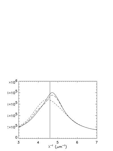
Figure 1: Cross section per unit volume, $C/V$, of randomly oriented $N=16$ CCA graphite clusters. Three different ways (see text) are used to treat the anisotropy of graphite: “1/3–2/3” approximation (long dashed line), random assignment (solid line), and averaged dielectric function (short dashed line). The vertical line marks the interstellar UV feature peak position

There are three distinct ways to deal with the anisotropy of graphite in the multiple Mie sphere code. The first way is to use the “1/3–2/3” rule, i.e. to average the extinction cross sections of the agglomerates with either $\epsilon_{\parallel}$ or $\epsilon_{\perp}$. The second way is to randomly assign $\epsilon_{\parallel}$ or $\epsilon_{\perp}$ with probabilities 1/3 and 2/3 to the individual spheres forming the aggregates. The third way is to average the components of the dielectric tensor and to use the resulting dielectric function in the multiple Mie sphere computations. These different approaches should be good approximations if we assume that there is no correlation between the orientations of the anisotropic spheres within the clusters and the direction of their individual c-axes. This is true for the regions outside of the resonance. However, it turns out that the results of the three methods differ from each other markedly in the bump region (Fig. 1). E.g. for the CCA cluster the averaged dielectric function (third way) leads to a much broader feature ($\gamma=2.20\,\mu{\rm m}^{-1}$) at smaller wavenumbers ($x_{\rm max}=4.48\,\mu{\rm m}^{-1}$) compared to the results obtained with the “1/3–2/3” rule (results for other arrangements of spheres are discussed in detail below) and the random assignment (second way). Furthermore, the feature obtained with the “1/3–2/3” rule shows a small shoulder in the long-wavelength wing. The appearance of the shoulder is explained by the rather long linear chains of the strong $\epsilon_{\perp}$ “oscillators”. In case of the random assignment the chains are interspersed by the weak $\epsilon_{\parallel}$ “oscillators” which makes the feature less sensitive to the detailed cluster structure (see Sect. 4.2). The averaged dielectric function (third way) is in any case also more or less moderate compared to $\epsilon_{\perp}$ regardless of the used averaging procedure. The feature position and width, however, certainly depend on the averaging procedure (the numbers given above are for the Bruggeman mixing rule; Bohren & Huffman 1983). Which way and which averaging procedure have to be used to get the best approximation of the $C/V$ of clusters of graphite spheres may be tested with extensive DDA calculations in the future, but this subject goes beyond the goals of this paper. In any case, one should note that more detailed information about the arrangement of basic structured units (in respect to their individual c-axes) from laboratory data are required to get a more reliable basis for the calculations (see Rouzaud & Oberlin 1989). The remaining discussion in this section is restricted to the results obtained with the “1/3–2/3” rule for the various sphere configurations.

\begin{picture}(0.0,6.2)\end{picture}

Figure 2: $C/V$ of a Rayleigh sphere (dotted line), a bisphere (dash-dotted line), a chain of three spheres (dash-triple-dot line), an $N=16$ CCA cluster (long dashed line), an $N=16$ compact cluster (solid line), and CDE (short dashed line). All arrangements of spheres are randomly oriented, using the “1/3–2/3” approximation to treat the anisotropy of graphite

Figure 2 shows $C/V$ for a single sphere, a randomly oriented bisphere, a randomly oriented linear chain of three touching spheres, a CCA cluster containing 16 spheres, and a compact cluster also containing 16 spheres. Other random realizations of these clusters, also containing 16 spheres, gave very similar results. In particular the shoulder observed around $4\,\mu{\rm m}^{-1}$ is reproduced in all CCA cluster realizations. The appearance of the UV feature looks very similar if only $C(\epsilon_{\perp})/V$ is plotted. Note that in going from a single sphere to chains of increasing $N$, the peak decreases in amplitude, while the extinction rises preferentially in the long-wavelength wing of the feature. The feature of a CCA cluster is similar to that of a chain of three spheres, except that this extinction enhancement has developed into a shoulder. Also shown for comparison (short dashed line) is $C/V$ for a continuous distribution of ellipsoids (CDE; Bohren & Huffman 1983), a widely used approximate clustering model.

Table 1: Computed and fitted $C/V$ peak position (“PEAK” and $x_{\rm max}$, respectively) and width (“FWHM” and $\gamma$, respectively) for arrangements of graphite spheres (in $\mu{\rm m}^{-1}$)

cluster	PEAK	FWHM	$x_{\rm max}$	$\gamma$	$\chi^{2}$
1 sphere	4.743	1.21	4.762	1.06	67.6
2 spheres	4.735	1.48	4.738	1.31	74.6
3 spheres	4.742	1.73	4.731	1.52	225.2
CCA	4.716	1.87	4.708	1.79	365.4
compact	4.696	1.61	4.680	1.48	34.9
CDE	4.268	2.46	4.332	2.40	21.4

Table 1 lists the peak position (“PEAK”), full-width at half-maximum (“FWHM”) of the computed $C/V$, as well as $x_{\rm max}$ and $\gamma$ derived from a fit similar in form to Eq. (1), with fitting coefficients $c_{1},\;c_{2},\;c_{3}$ and $c_{4}$, using a slightly modified version of the routine given in Fitzpatrick & Massa (1990). To indicate the degree of quality of the fit, the $\chi^{2}$ value (in units of $10^{6}$) is also given, which is defined in the usual way with the weight for each $C/V$ data point (sampled at uniform intervals in wavenumber) set to the (arbitrary) value 1 except for the bump region $x=3.3$–$5.9\,\mu{\rm m}^{-1}$ where the weight is set to 2. Apart from the CDE case (which turns out to be a bad clustering model for the bump), the parameter $x_{\rm max}$ is quite stable ($\la 1.7\%$ relative variation), whereas $\gamma$ is substantially increased (by $40-70\%$) in going from a single sphere to clusters. These features satisfy qualitatively the observational constraints, except for the fact that the peak position is wrong ($\sim 4.68$–$4.76\,\mu{\rm m}^{-1}$ compared to $4.60\pm 0.04\,\mu{\rm m}^{-1}$). Note that there is a significant difference between “PEAK” and $x_{\rm max}$, and between “FWHM“ and $\gamma$. This is due to the fact that a Drude profile fit is applied to a profile that is not purely Drude-like, thus introducing a spurious linear background (coefficients $c_{1}$, $c_{2}$) which modifies both the peak position and the width of the feature. The fit in the case of the compact cluster is reasonable, which is indicated by the small $\chi^{2}$ value in Table 1, whereas the fit is somewhat poorer in the case of the CCA cluster (due to the presence of the shoulder), yielding a larger $\chi^{2}$.

The peak position is at a larger wavenumber than that observed for the interstellar UV feature. This is why one has to resort to either shape or size effects to shift the feature at the position of the interstellar UV feature (see, e.g., Draine 1988; Mathis 1994). Discounting the disagreement in peak position and concentrating only on the qualitative aspect of the feature, one can surmise that some irregularly shaped or clustered particles can in fact broaden the feature without appreciably shifting its peak position, as required for the purported interstellar UV feature carrier. However, “fluffy” or elongated structures tend to enhance the long wavelength wing of the feature, even introducing additional structure in the feature (like the CCA cluster does). Assuming this is a general feature of CCA clusters (see Sect. 4), it then appears that fluffy particles are severely constrained as a possible “topology” of the interstellar UV feature carrier. A compact cluster is an appealing alternative, since its overall spherical shape and compactness suppresses the appearance of additional structure in the feature, but still allows the feature to be broadened substantially compared to isolated spheres. The broadening, however, appears to be insufficient to explain all the range of FWHM observed for the interstellar UV feature. A further contributor to the broadening could be an intrinsic variability in chemical composition. This interpretation is consistent with the fact that the narrowest interstellar UV features appear in all sorts of environments, diffuse and dense alike, with an accompanying variation in peak position over the whole observed range. We expect a clustering of grains to occur primarily in denser regions. The ensuing broadening, however, appears to contradict the observation that the broadest interstellar UV features (observed in dense regions and thus presumably arising from clustering) are accompanied by a shift of $x_{\rm max}$ to larger values, whereas here, it shifts to smaller values (see Table 1). But this does not necessarily need to be the case, as shown in the following section.

4 Single-Lorentz oscillator models

Actually, in view of the widely assumed formation mechanisms of the carbonaceous component responsible for the UV bump, the highly anisotropic dielectric function of planar graphite is unlikely to be a good model of the purported dielectric function of the bump carrier. First, the exposure of the carbonaceous interstellar grains to UV radiation, though conducive to a “graphitization” of the material through dehydrogenation, is unlikely to produce perfect graphite sheets as an end-product (Sorrell 1990). There must still be considerable defects in the structure, the topology of the grains being a collection of randomly oriented graphitic crystallites in a sp³ bonding matrix (possibly containing some hydrogen). This structure is more characteristic of amorphous carbon (especially UV processed or annealed hydrogenated amorphous carbon — HAC; Fink et al. 1984; Mennella et al. 1995a,b). Furthermore, modification of the optical constants of graphite have already been shown to be necessary in order to reproduce even the most basic properties of the interstellar UV feature (Mathis 1994). An intrinsic variability in chemical composition must also be considered in order to satisfy the observational constraints.

Virtually all UV bumps observed to date can be reproduced extremely well by a “Drude” profile. This is the profile generated by a sphere whose optical properties are characterized by a single-Lorentz oscillator model. Thus, in this section, we consider a single-Lorentz oscillator model to approximate the dielectric function hypothesized for the interstellar UV feature carrier, and see how shape and clustering can affect the peak position, width, and shape of the UV bump. We assume that variability in the width is attributable to shape and clustering effects, as well as to intrinsic variations in chemical composition along different lines of sight. Variability in the peak position, which is observed to be uncorrelated with width, is attributed to variations in mean chemical composition alone.

The dielectric function of a Lorentz oscillator is given by $\epsilon=1+x_{p}^{2}/[x_{0}^{2}-x^{2}-i\gamma_{0}x]$, where $x_{p}$, $x_{0}$, and $\gamma_{0}$, are the plasma frequency, the peak position, and the damping constant, respectively, all in units of the inverse wavelength ($\mu{\rm m}^{-1}$). A Drude model is characterized by $x_{0}=0$ and usually describes metals (or semi-metals, like graphite). Through these parameters, the model can simulate the variability of the chemical composition of the grains and provide some physical insight into the mechanisms involved.

Interstellar grains cannot be expected to be perfectly smooth spheres in all environments. For example, one may expect aggregation of the primary grains, especially in denser regions. Furthermore, the grains could be characterized by surface roughness and/or by porosity, as well as chemical inhomogeneities. An interesting question is whether such shape and clustering effects (neglecting chemical inhomogeneities within a given grain) can conserve the Drude-like profile that is observed, along with the other observational constraints.

4.1 Combining a Lorentz oscillator model with shape and clustering

The effect of shape and clustering on the scattering properties of chemically homogeneous grains in the Rayleigh limit can be modelled via a spectral density, $g(L)$, of the geometric factor $L$, where $0\leq L\leq 1$ (Bohren & Huffman 1983; Fuchs 1987; Rouleau & Martin 1991). The requirements are that the zeroth and first moments of $g(L)$ are unity and $1/3$, respectively. This approach is closely related to the “Bergman representation” which is based on effective medium theory in the case of a binary mixture (Stognienko et al. 1995). The two approaches are equivalent if one assumes that one of the components is vacuum. However, the spectral density $g(L)$ can be directly interpreted in terms of shape and clustering of small grains, whereas the Bergman representation deals with bulk material, and so gives only indirect information about the scattering properties of small grains.

Combining a single-Lorentz oscillator model of dielectric function $\epsilon=1+x_{p}^{2}/[x_{0}^{2}-x^{2}-i\gamma_{0}x]$ with a model of shape and clustering using $g(L)$, the extinction cross section per unit volume can be written as

$$\frac{C}{V} = 2\pi\,x\,{\rm Im}\int_{0}^{1}\frac{g(L)\,dL}{(\epsilon-1)^{-1}+L}$$

$$= 2\pi\int_{0}^{1}\frac{x_{p}^{2}\gamma_{0}g(L)\,dL}{\left[x-(x_{0}^{2}+x_{p}^{2}L)/x\right]^{2}+\gamma_{0}^{2}}$$

where ${\rm Im}$ denotes the imaginary part. The familiar form of $C/V$ for spheres is obtained from $g(L)=\delta(L-1/3)$. Note that $C/V$ using this model has the form of the “bump” term in Eq. (1) if $g(L)=\delta(L-L_{o})$. In that case, the maximum $C/V$ occurs close to

$$x_{\rm max}=[x_{0}^{2}+x_{p}^{2}L_{o}]^{1/2}.$$ (3)

One advantage of this type of representation is that a statistical ensemble of grains of various shapes or clustering states can also be represented by an average $g(L)$. Actually some mean $g(L)$ and mean $\epsilon$ could even describe qualitatively a statistical ensemble of grains with varying shape and chemical composition, as long as there are no correlations between the two.

The irregular grains considered here arise from the agglomeration of spheres (i.e. the spheres can touch their neighbour at one point, but they are not allowed to interpenetrate). In the case of agglomerates of spheres, the spectral representation approach brings about a considerable reduction in computer burden compared to direct computations using a multiple Mie sphere code since the problem has to be solved only once. Results between the two approaches in the case of clusters of spheres using the optical constants of graphite are very similar.

To compute the spectral density $g(L)$ we use a code kindly provided by Hinsen & Felderhof (1992). This code computes ensemble-averaged electromagnetic interactions between identical spheres in the electrostatic limit. As stated in Stognienko et al. (1995), the spectral density depends on the choice of the maximum order for the multipole expansion. We present the spectral densities computed with multipole expansion order of 9 for the $N=16$ CCA clusters and the $N=16$ compact clusters in Fig. 3. Note that a multipole expansion order of 6 is sufficient to obtain convergence for the $C/V$ results using Eq. 4.1 with the optical constants of graphite.

\begin{picture}(0.0,6.3)\end{picture}

Figure 3: Spectral density for $N=16$ CCA clusters (dashed line) used in Fig. 4, and spectral density for $N=16$ compact clusters (solid line) used in Fig. 5. The vertical line represents the spectral density of spheres, a delta function at $L=1/3$

For our simple Lorentz model, we assign one of the smallest widths derived from interstellar extinction curves, $\gamma=0.77$ (for HD 93028; Fitzpatrick & Massa 1986), to spheres. This might not be completely correct, but the sphere is a useful reference shape. We assume here that broader widths arise exclusively from shape and clustering effects without any variation in chemical composition. We choose the peak position as being the mean value, $x_{\rm max}=4.60\,\mu{\rm m}^{-1}$. This is an arbitrary choice since the narrowest profiles ($\gamma<0.8$) span almost the entire range of $x_{\rm max}$, from $4.58\,\mu{\rm m}^{-1}$ to $4.62\,\mu{\rm m}^{-1}$. Other choices of $x_{\rm max}$ would yield qualitatively similar results, but simply shifted in wavenumber. These would correspond to intrinsic variations of the assumed chemical composition of the grains.

For spheres, a pure Drude profile is obtained. Due to shape and clustering effects, however, the synthetic bump computed from $g(L)$ may differ from a pure Drude profile. We wish to find out under which conditions such clustering models can produce an increase in width of the bump without appreciably changing its peak position or its Drude-like shape.

\begin{picture}(0.0,13.6)\end{picture}

Figure 4: $C/V$, $\epsilon_{r}$, and $\epsilon_{i}$, for various single-Lorentz oscillator models and the $g(L)$ computed from $N=16$ CCA clusters. By order of increasing amplitude, the models are given by $x_{0}=4.0,\;3.6,\;3.2,\;2.4,$ and 0.0 (solid lines). The dotted lines are the fit using Eq. (1)

Table 2: Same as Table 1 but for single-Lorentz oscillator models parameterized by $x_{0}$ in the case of $N=16$ CCA clusters (PEAK $=x_{\rm max}=4.60$ and FWHM $=\gamma=0.77$ for spheres). “MAX” (cm^-1) is the computed peak value $(C/V)_{\rm max}$

$x_{0}$	MAX	PEAK	FWHM	$x_{\rm max}$	$\gamma$	$\chi^{2}$
4.59	2.26E4	4.600	0.77	4.600	0.77	0.0
4.50	2.21E5	4.601	0.78	4.600	0.78	0.0
4.20	7.64E5	4.611	0.92	4.601	0.93	28.5
4.00	1.02E6	4.629	1.06	4.605	1.09	139.8
3.80	1.23E6	4.652	1.20	4.612	1.27	402.9
3.60	1.40E6	4.674	1.33	4.624	1.47	—
3.40	1.54E6	4.694	1.45	4.639	1.69	—
3.20	1.67E6	4.712	1.55	4.657	1.91	—
2.80	1.87E6	4.744	1.64	4.703	2.35	—
2.40	2.03E6	4.771	1.60	4.744	2.65	—
2.00	2.16E6	4.793	1.60	4.744	2.52	—
1.60	2.26E6	4.811	1.62	4.723	1.78	—
1.20	2.33E6	4.826	1.64	4.738	1.44	—
0.80	2.38E6	4.836	1.65	4.752	1.31	—
0.40	2.41E6	4.842	1.66	4.761	1.25	—
0.00	2.42E6	4.844	1.66	4.764	1.24	—

4.2 Results for CCA clusters

Figure 4 shows the extinction cross section per unit volume, $C/V$, and the real and imaginary part of the dielectric function, $\epsilon_{r}$ and $\epsilon_{i}$, for various single-Lorentz oscillator models using the $g(L)$ computed from $N=16$ CCA clusters. The models were parameterized using $x_{0}$ and $x_{p}=[3(4.60^{2}-x_{0}^{2})]^{1/2}$. This choice of $x_{p}$ gives rise to a peak at $4.60\,\mu{\rm m}^{-1}$ for spheres ($L_{o}=1/3$ in Eq. [3]). The damping constant is set to $\gamma_{0}=0.77\,\mu{\rm m}^{-1}$. For spheres, this produces a Drude profile of width $\gamma=0.77\,\mu{\rm m}^{-1}$.

In order of increasing amplitude, results shown are for $x_{0}=4.0,\;3.6,\;3.2,\;2.4,$ and 0.0 (solid lines). Also shown for comparison are the fits using the procedure of Fitzpatrick & Massa (1990; dotted lines). Note the considerable amount of structure in the profiles, except for the weakest model shown, $x_{0}=4.0$. The corresponding $g(L)$ is shown in Fig. 3 (dashed line). A comparison between the two figures indicates that the $C/V$ of models with the smallest $x_{0}$ (“strong” Lorentz models, i.e. closest to a Drude model) are just a convolution of $g(L)$ with a broadened Drude profile. Thus, for “strong” Lorentz models, extra peaks in the profile of $g(L)$ will translate into structure in the $C/V$ curves. Conversely, for “weak” Lorentz models ($x_{p}^{2}L\ll x_{0}^{2}$ in Eq. [4.1]) the profile will be close to a “Drude” profile, irrespective of the form of $g(L)$.

Table 2 is similar to Table 1, but for the one-Lorentz oscillator models using the $g(L)$ of CCA clusters. In the present case, $x_{\rm max}$ and $\gamma$ are meaningless for $x_{0}\la 3.8$ since the curves are poorly represented by a “Drude” profile (thus being inconsistent with observations of actual interstellar extinction curves). Again, note the significant discrepancies between “PEAK” and $x_{\rm max}$, and between “FWHM” and $\gamma$ because of the spurious fitted linear rise. Only $\chi^{2}$ values of less than 500 are listed, corresponding to models that are acceptable. Note that, though the curves are not strictly Drude-like, “PEAK” shifts to larger values compared to that of spheres (4.60$\,\mu{\rm m}^{-1}$) for broader profiles, precisely what is observed in denser interstellar environments. This is related to the fact that the $g(L)$ profile peaks at a value of $L$ larger than 1/3 (the value of $L$ for spheres, indicated by a vertical line in Fig. 3).

The ratio of carbon locked up in interstellar grains relative to hydrogen, $N_{\rm C}/N_{\rm H}$, is thought be be around $\sim 100$ part-per-million (ppm) by number (Cardelli et al. 1996). Assuming the bump grains have a density of 2 g cm^-3, then only the “weakest” Lorentz models ($x_{0}\ga 4.5$) require more carbon than available (cf. the values of $(C/V)_{\rm max})$ in Table 2). As expected, putting all the carbon in a single extinction feature requires only modest amounts of the element.

Thus cluster-cluster agglomeration (i.e. fluffy interstellar grains) can reproduce the observational constraints relating to the interstellar UV feature, provided the bump grains are described by a single-Lorentz oscillator model with $x_{0}\sim 3.8$–$4.5\,\mu{\rm m}^{-1}$.

\begin{picture}(0.0,13.6)\end{picture}

Figure 5: Same as Fig. 4, but for a $g(L)$ computed from $N=16$ compact clusters (solid line in Fig. 3)

Table 3: Same as Table 2, but in the case of $N=16$ compact clusters

$x_{0}$	MAX	PEAK	FWHM	$x_{\rm max}$	$\gamma$	$\chi^{2}$
4.59	2.25E4	4.600	0.77	4.600	0.77	0.0
4.50	2.23E5	4.600	0.78	4.600	0.78	0.0
4.20	7.86E5	4.597	0.88	4.598	0.88	12.0
4.00	1.07E6	4.596	0.99	4.595	0.99	54.6
3.80	1.29E6	4.600	1.10	4.592	1.12	125.7
3.60	1.47E6	4.607	1.20	4.590	1.25	213.9
3.40	1.61E6	4.616	1.31	4.590	1.39	318.1
3.20	1.73E6	4.626	1.41	4.591	1.53	448.2
2.80	1.91E6	4.650	1.60	4.597	1.83	—
2.40	2.05E6	4.673	1.76	4.609	2.12	—
2.00	2.15E6	4.693	1.89	4.627	2.40	—
1.60	2.22E6	4.712	1.99	4.649	2.67	—
1.20	2.27E6	4.726	2.07	4.671	2.88	—
0.80	2.31E6	4.736	2.13	4.691	3.05	—
0.40	2.33E6	4.742	2.16	4.704	3.15	—
0.00	2.34E6	4.744	2.17	4.709	3.19	—

4.3 Results for compact clusters

We also computed $C/V$ using Eq. (4.1) for a $g(L)$ corresponding to an ensemble of compact clusters containing $N=16$ spheres. Figure 5 is similar to Fig. 4, but for an ensemble of $N=16$ compact cluster models. The corresponding $g(L)$ is shown in Fig. 3 (solid line). Note that the $g(L)$ of compact clusters also peaks at $L>1/3$, but that it is more “compact” and contains less structure than the $g(L)$ of CCA clusters. This translates into $C/V$ profiles that are closer to a Drude profile, except again for “stronger” Lorentz models ($x_{0}\la 3.6$). This emphasizes how tightly constrained the shape and clustering of grains described by the stronger single-Lorentz oscillator models are in terms of their allowable $g(L)$ profile. Table 3 lists the same parameters as Table 2 for the various compact clusters using these Lorentz models. Models with $3.2\la x_{0}\la 4.5$ satisfy most of the observational constraints. Only models with $x_{0}\ga 4.5$ violate the cosmic carbon abundance constraint. Note again the trend of larger FWHM’s usually leading to larger values of “PEAK”, as required observationally.

5 Two-Lorentz oscillator models

The simple approach taken in the previous section – to model the optical properties of the interstellar UV feature carrier with a single Lorentz oscillator – may appear somewhat unrealistic. It assumes that the bump carrier does not contribute at all to the FUV rise. Actually, along some lines of sight (many passing through Orion), the FUV rise is observed to be very small or virtually absent, even though the interstellar UV feature is still present, albeit weaker than usual. But all carbonaceous materials (including diamond) are expected to give rise to a peak at roughly 10–15$\,\mu{\rm m}^{-1}$ due to the $\sigma$–$\sigma^{*}$ electronic transition (Mennella et al. 1995a; Fink et al. 1984). Moreover, any plausible material in the small particle limit will produce strong absorption at $x>6\,\mu{\rm m}^{-1}$.

To our knowledge, no physical mechanism can suppress the $\sigma$–$\sigma^{*}$ transition while keeping intact the $\pi$–$\pi^{*}$ transition responsible for the UV feature. Thus, the assumption that the UV bump carrier is carbonaceous in nature appears at first glance to be difficult to reconcile with the very small FUV rise observed in a number of cases. In this section, we ignore this difficulty and assume that the dielectric function of the interstellar UV feature carrier is the sum of two Lorentz oscillators – one producing the UV bump, and the other producing the FUV curvature– to see how the conclusions of the preceding section are modified.

One important distinction must be made here. If two grain populations are unrelated, then one can add their cross sections, like is implicit in the decomposition of Eq.(1). For example, adding an extra linear background or an extra FUV curvature will affect only their corresponding fitting parameters in Eq. (1), but will leave the other fitting parameters unchanged. However, if the UV bump and the FUV curvature arise from the same parent material, then their respective contributions to the total dielectric function must be added instead, and then only can the cross section be computed assuming a certain grain shape. These various contributions to the dielectric function do not necessarily add up linearly when translated into cross sections, unless $\epsilon_{i}$ is small. Therefore, adding an extra Lorentz oscillator at larger $x$ (in $\epsilon$ space) to an initial one that produces a UV bump well characterized by a “Drude” profile (for example, assuming a spherical shape) might actually result into a bump that is no longer Drude-like. As a result of this process, all fitting parameters may be affected in a non-trivial way.

To investigate these effects we approximate such a dielectric function as the sum of two Lorentz oscillators, giving rise to features at about $4.6\,\mu{\rm m}^{-1}$ (the UV bump) and 10–15$\,\mu{\rm m}^{-1}$ (the FUV bump), respectively. This guarantees that the total dielectric function of the material satisfies Kramer-Kronig relations (Bohren & Huffman 1983). Of course, more complicated dielectric functions are also possible, but then the number of free parameters becomes rapidly excessive, and the physical interpretation becomes less straightforward.

\begin{picture}(0.0,13.6)\end{picture}

Figure 6: Same format as Figs. 4 and 5, but for various Lorentz oscillator models and for spheres. Results shown are for a single-UV-Lorentz oscillator model with $x_{01}=4.0$, $x_{p1}=3.934$, $\gamma_{01}=0.77$ (dotted lines), and for models involving an extra FUV Lorentz oscillator with $x_{02}=10.0$, $x_{p2}=6.833$, and $\gamma_{02}=0.3$ (solid lines), 3.0 (dashed lines), 6.0 (dash-dotted lines), and 12.0 (dash-triple-dot lines)

The effects of this extra Lorentz oscillator on the UV bump are illustrated in Fig. 6. The UV oscillator is given by the parameters $x_{01}=4.0$, $x_{p1}=3.934$, and $\gamma_{01}=0.77$, which on its own yields a $C/V$ peak at 4.60$\,\mu{\rm m}^{-1}$ assuming a sphere (dotted line). The FUV oscillator is given by $x_{02}=10.0$, $x_{p2}=6.833$, and various widths, which on its own yields a $C/V$ peak at $10.75\,\mu{\rm m}^{-1}$ assuming a sphere. This could be viewed as a very crude model of the $\sigma$–$\sigma^{*}$ peak observed for HAC in laboratory extinction experiments (Mennella et al. 1995a). The solid, dashed, dash-dotted, and dash-triple-dot lines are for $\gamma_{02}=0.3,\;3.0,\;6.0$, and 12.0, respectively (also assuming spheres). The main effect of the FUV oscillator is to decrease the strength of the UV bump, more or less independently of the width of the FUV bump (keeping the FUV oscillator strength constant). Another effect is to shift the peak position of the UV bump to smaller wavenumbers ($4.506,\;4.519,\;4.536$, and 4.573$\,\mu{\rm m}^{-1}$, for $\gamma_{02}=0.3,\;3.0,\;6.0$, and 12.0, respectively). An extra broadening also occurs, but only on the larger $x$ wing of the bump. Changing the width of the FUV oscillator without changing its strength affects the FUV curvature dramatically. Actually, this suggests an explanation for the quasi-absence of FUV curvature observed along some lines of sight: if the FUV bump is extremely narrow (or shifted to large enough wavenumbers), then the FUV rise may be virtually absent (solid line). This is also obtained for very wide FUV bumps, but then there is a “jump” in the linear component of the extinction across the UV bump (dash-triple-dot line). However, Fitzpatrick & Massa (1988) have shown that the linear background of interstellar extinction curves, once the fitted bump has been subtracted out, is very smooth across the bump, with no evidence of jumps or changes of slope. Therefore extremely broad FUV bumps are more or less ruled out as an explanation of the lack of a FUV curvature concurrent with the presence of a UV bump.

The main effect of adding such a background to the dielectric function is to increase $\epsilon_{r}$ and, to a lesser extent, $\epsilon_{i}$, shifting the plasmon condition ($\epsilon_{r}<0$) to smaller wavenumbers. Note how little the dielectric function of the UV oscillator is changed for smaller wavenumbers when changing the width of the FUV oscillator (keeping the strength constant).

When a shape different from a sphere is assumed (either a CCA or a compact cluster), as a result of this extra background, the peak position is shifted to smaller wavenumbers, contrary to what was obtained in the previous section. A moderate increase in FWHM is also obtained. These results are similar to what was obtained in the case of graphite (Table 1).

\begin{picture}(0.0,6.3)\end{picture}

Figure 7: $C/V$ of Mie spheres for various radii $a$ using the dielectric function with $\gamma_{02}=3.0$ in Fig. 6 (dashed lines). In order of decreasing strength, $C/V$ for radius $a$ in the Rayleigh limit, and $a=0.01,\;0.02,\;0.03,\;0.04,\;0.05,$ and 0.1 $\mu$m, respectively

5.1 The effect of scattering on the FUV curvature

Another mechanism that can flatten the FUV bump is scattering by larger grains. But scattering is likely to affect the UV feature as well (mainly shifting it to smaller wavenumbers – which is not observed in all interstellar cases), unless a size distribution could be such that it would affect only wavenumbers larger than $\sim 4.6\,\mu{\rm m}^{-1}$. However, this is unlikely, as shown in Fig. 7. Plotted (in order of decreasing strength) are the $C/V$ Mie curves for spheres with radius $a$ in the Rayleigh limit, and $a=0.01,\;0.02,\;0.03,\;0.04,\;0.05,$ and 0.1 $\mu$m, respectively, using the dielectric function with $\gamma_{02}=3.0$ in Fig. 6 (dashed lines). Note that the UV bump is strongly affected in peak position and shape for $a\ga 0.03~{}\mu$m, even though the FUV peak is still quite large (with much FUV curvature). The size which produces a FUV bump that is essentially flat, $a=0.1~{}\mu$m (lowest curve), also yields a UV bump that is virtually unrecognizable. Here, the UV peak is more strongly affected than the FUV peak because the dielectric function in the UV range is closer to a plasmon condition (see Fig. 6). Therefore, a size distribution of grains (weighting these curves by the volume of individual grains) is unlikely to flatten the FUV rise without severely affecting the shape and peak position of the UV bump as well.

5.2 Synthetic interstellar extinction curves

A direct comparison between the fitting parameters of interstellar curves and some synthetic ones can be useful to assess the qualities of the Drude profile for the UV bump and the term $f_{\rm FUV}(x)$ for the FUV curvature when two-Lorentz oscillator models are considered. To make such a comparison, a few simplifying assumptions are required. The total optical depth is assumed to arise from two contributions, one from grains producing most of the linear rise between 3 and 8.5$\,\mu{\rm m}^{-1}$ (labelled $l$) and one from the grains producing the bump, the rest of the linear rise, and the FUV curvature (labelled $b$). The component $l$ is assigned to silicate grains. The lack of correlation between the linear rise parameters and the bump parameters suggests that the grains responsible for the UV bump do not contribute appreciably to the linear rise (Jenniskens & Greenberg 1993). Thus assigning most of the linear rise to silicate grains is reasonable. The different slopes observed in the interstellar extinction curves (see, e.g., Fig. 8) could be assumed to arise from different size distributions of silicate grains (with larger mean grain sizes producing flatter curves). For the sake of simplicity, we shall not be concerned here with the detailed modelling of this component, but will simply assume that its $C/V$ can be described as a simple linear rise in the range 3–8.5$\,\mu{\rm m}^{-1}$. For the carbonaceous component $b$, a key normalization parameter is the carbon to hydrogen ratio (by number), $N_{\rm C}/N_{\rm H}$.

\begin{picture}(0.0,13.6)\end{picture}

Figure 8: $A(x)/A_{\rm V}$, $\epsilon_{r}$, and $\epsilon_{i}$, for various Lorentz oscillator models assuming spheres. The parameters of the models, listed in Table 4, were chosen to fit actual interstellar curves (solid lines). Models are for HD 204827 (dotted lines), HD 229196 (dashed lines), and HD 37023 ($\theta^{1}$ Ori D; dash-dotted lines: thick—$N_{\rm C}/N_{\rm H}=90$ ppm, thin—45 ppm)

Assuming $A_{\rm V}=1.7\times 10^{-22}N_{\rm H}R_{\rm V}$ (Mathis 1994) and using $A(x)=1.086(N_{l}C_{l}+N_{b}C_{b})$, where $N_{j}$ is the column density of dust and $C_{j}$ is the cross section of component $j$ (where $j=l,\,b$), we have from the definition of $k(x)$,

$$k(x) = R_{\rm V}\frac{A(x)}{A_{\rm V}}-R_{\rm V}$$

$$= \frac{1.086}{1.7\times 10^{-22}}\frac{N_{b}}{N_{\rm H}}\left[\frac{N_{l}}{N_{b}}C_{l}(x)+C_{b}(x)\right]-R_{\rm V},$$

where $R_{\rm V}=A_{\rm V}/E$(B-V) is the total-to-selective extinction ratio in the V band. We have $N_{b}\simeq 12m_{\rm H}N_{\rm C}/(\rho_{b}V_{b})$, where $m_{\rm H}$ is the mass of the hydrogen atom, and $\rho_{b}$ and $V_{b}$ are the density and the mean volume of the grains, respectively. The density of bump grains is again assumed to be $2\,{\rm g}{\rm cm}^{-3}$. The computed cross section per unit volume of the bump grains using two Lorentz oscillators (i.e. seven free parameters: $x_{0j}$, $x_{pj}$, $\gamma_{0j}$, $j=1,2$, and $N_{\rm C}/N_{\rm H}$) is fitted by

$$\frac{C_{b}(x)}{V_{b}}=c_{b1}+c_{b2}x+\frac{c_{b3}}{(x-x_{\rm max}^{2}/x)^{2}+\gamma^{2}}+c_{b4}f_{\rm FUV}(x)\\$$

between 3 and 8.5$\,\mu{\rm m}^{-1}$. Assuming that $C_{l}(x)$ is linear with respect to $x$, Eq. (5.2) can be rewritten as

$$k(x)=R_{\rm V}C_{0}\left[c_{l1}+c_{l2}x+\frac{C_{b}(x)}{V_{b}}\right]-R_{\rm V},$$ (5)

where $c_{l1}=(a_{1}+R_{\rm V})/(R_{\rm V}C_{0})-c_{b1}$, $c_{l2}=a_{2}/(R_{\rm V}C_{0})-c_{b2}$, and $R_{\rm V}C_{0}\simeq 0.064N_{\rm C}/N_{\rm H}$.

Interstellar extinction curves along specific lines of sight were modelled using this two-Lorentz oscillator model assuming Rayleigh spheres over the whole range. Using the same optical constants and the same normalization, results for CCA clusters and compact clusters were also computed to see how the bump parameters changed. Uncertainties related to the extrapolation beyond the observed range (3–8.5$\,\mu{\rm m}^{-1}$) do not warrant taking the extra complication of scattering into account. The value of $N_{\rm C}/N_{\rm H}$ was set more or less arbitrarily to 90 ppm (i.e. slightly below the current derived limit) and to 45 for the line of sight where a weak UV bump is observed (case of HD 37023). Smaller values than 90 ppm for the other two lines of sight would require more extreme Lorentz oscillator parameters and extinction curves may exhibit some substructure (see Fig. 4), and so it might be more difficult to obtain a good fit.

Figure 8 shows $A(x)/A_{\rm V}$ for spheres using $\epsilon_{r}$ and $\epsilon_{i}$ (shown in the middle and bottom panels, respectively). The dielectric function was computed from the parameters of two-Lorentz oscillator models. These parameters, listed in Table 4, were chosen to reproduce (assuming spheres) the extinction along three lines of sight spanning a wide range in FUV curvature (Fitzpatrick & Massa 1988; 1990). The lines of sight are in the direction of HD 204827 (top solid line, modelled by the dotted lines), HD 229196 (middle solid line, modelled by the dashed lines), and HD 37023 ($\theta^{1}$ Ori D; lower solid line, modelled by the dash-dotted lines). The values of $R_{\rm V}$ were taken from Cardelli et al. (1989). In Table 5, the resulting fitting parameters obtained for spheres, CCA clusters and compact clusters are compared to those of these interstellar extinction curves. As can be shown by the $\chi^{2}$ values (relative to $C/V$, not $A/A_{\rm V}$; in units of $10^{6}$), the fit is excellent. Surprisingly, the fit can actually improve in going from spheres to clusters (case of HD 204827). This is mainly due to a better fit of the FUV curvature, not the UV bump. In case of HD 37023 the fit becomes slightly worse (due to a slight FUV curvature mismatch) in reducing $N_{\rm C}/N_{\rm H}$ from 90 to 45 ppm. Both oscillators are shifted to smaller wavenumbers in case of $N_{\rm C}/N_{\rm H}=45$ ppm, and, as expected, the fitted UV oscillator appears to be much stronger (larger $x_{p1}$) than for the case of 90 ppm. Interestingly, $\gamma_{01}$ is even more reduced in case of 45 ppm. At any rate, the $\chi^{2}$ values are usually smaller than in the single-Lorentz oscillator case (see entries $x_{0}=4.0$ in Tables 2 and 3). Thus it appears that an extra background under the UV bump (due to the FUV oscillator contribution to the UV oscillator) makes the bump profile less sensitive to shape and clustering.

Table 4: Parameters of two-Lorentz oscillator models to reproduce interstellar extinction curves along selected lines of sight

	$x_{01}$	$x_{p1}$	$\gamma_{01}$	$x_{02}$	$x_{p2}$	$\gamma_{02}$	$c_{l1}$$\times$$10^{6}$	$c_{l2}$$\times$$10^{6}$	$N_{\rm C}/N_{\rm H}$ (ppm)	$R_{\rm V}$
HD 204827	4.100	4.200	1.060	8.200	7.400	2.900	0.369	0.151	90	2.60
HD 229196	4.105	3.890	0.980	9.700	7.400	2.350	0.570	0.105	90	3.12
HD 37023	4.407	2.425	0.890	10.200	7.400	2.350	1.265	$-$0.028	90	5.23
HD 37023	4.203	3.553	0.868	9.400	7.400	2.350	2.522	$-$0.052	45	5.23

Table 5: Fitting parameters of synthetic interstellar extinction curves compared to actual ones

	$N_{\rm C}/N_{\rm H}$ (ppm)	$x_{\rm max}$	$\gamma$	$a_{1}$	$a_{2}$	$a_{3}$	$a_{4}$	$\chi^{2}$
HD 204827		4.623	1.070	$-$1.521	1.219	3.201	0.899
sphere	90	4.623	1.075	$-$1.521	1.219	3.200	0.882	46.9
CCA	90	4.553	1.166	$-$1.575	1.235	3.701	0.871	15.1
compact	90	4.575	1.127	$-$1.561	1.231	3.495	0.880	15.5
HD 229196		4.581	0.990	$-$0.179	0.728	3.407	0.233
sphere	90	4.582	0.991	$-$0.179	0.728	3.410	0.234	9.2
CCA	90	4.541	1.128	$-$0.213	0.723	4.263	0.271	14.6
compact	90	4.552	1.078	$-$0.211	0.726	3.951	0.257	10.0
HD 37023		4.594	0.878	1.883	$-$0.083	1.215	0.153
sphere	90	4.594	0.879	1.883	$-$0.083	1.215	0.153	2.1
CCA	90	4.579	0.903	1.879	$-$0.083	1.289	0.164	2.5
compact	90	4.583	0.895	1.880	$-$0.083	1.263	0.160	2.4
sphere	45	4.594	0.878	1.883	$-$0.083	1.215	0.153	18.1
CCA	45	4.558	0.977	1.870	$-$0.084	1.465	0.173	20.8
compact	45	4.568	0.941	1.872	$-$0.083	1.373	0.166	18.9

Unfortunately, given the already large number of free parameters (7), the models are not unique. But they give a qualitative idea of what the optical constants of actual bump grains might look like in various environments. Note that for curves exhibiting less FUV curvature, the second Lorentz oscillator must be shifted to larger $x$, otherwise the fit can be very poor in the FUV portion of the observed range. The FUV curvature observed in the direction of HD 204827 is so large ($a_{4}=0.899$) that no FUV Lorentz oscillator with $x_{02}\simeq 10\,\mu{\rm m}^{-1}$ can reproduce it (these tend to give $a_{4}\la 2.2$). These large curvatures can only be generated by bringing the FUV oscillator closer to the UV oscillator ($x_{02}\sim 8\,\mu{\rm m}^{-1}$). The fit is slightly poorer in that case for spheres since the tail of the FUV Lorentz oscillator significantly differs from the shape of this curvature. The bump peak position, $x_{\rm max}$, is sensitive mainly to $x_{01}$ (a $1\%$ variation in $x_{01}$ produces a $0.8\%$ variation in $x_{\rm max}$ – which is a substantial part of the observed range of variation of $x_{\rm max}$), and to a lesser extent, $x_{p1}$. The bump strength $a_{3}$ is sensitive to $x_{02}$ and $x_{p1}$, whereas the curvature $a_{4}$ is sensitive to $x_{02}$. Table 5 also shows that clustering, though still broadening the UV bump compared to spheres, systematically shifts the peak position of the bump to smaller wavenumbers, which is contrary to what was found for single-Lorentz oscillator models (and contrary to observations). Thus, the inclusion of a background dielectric function (arising from the oscillator associated with the FUV peak) inhibits the conditions under which a shift to larger wavenumbers is possible. Therefore, if the optical constants of Fig. 8 are representative of the interstellar UV feature carrier, then intrinsic variations in chemical composition, rather than clustering, may be responsible for this shift.

6 Physical mechanisms of relevance

In this section we discuss some of the laboratory studies examining the UV properties of some carbonaceous materials of astrophysical relevance and assess their usefulness in interpreting the results of the preceding sections.

Fink et al. (1984) have derived $\epsilon_{i}$ of HAC thin films for various annealing temperatures, $T_{a}$. As $T_{a}$ was increased, the $\pi$–$\pi^{*}$ peak (associated with sp² bonding) shifted to smaller wavenumbers and its strength increased. Equating a larger $T_{a}$ with less hydrogenation, this means that we expect $x_{01}$ to shift to smaller values and $x_{p1}$ to increase as the hydrogen content decreases. Figures 4 and 5 show qualitatively that trend. On the other hand, as $T_{a}$ was increased, the $\sigma$–$\sigma^{*}$ peak (observed for virtually all carbonaceous materials, including diamond) initially at $\sim 10\,\mu{\rm m}^{-1}$, shifted to larger wavenumbers ($\sim 11\,\mu{\rm m}^{-1}$ at $T=540^{\circ}$C), but its strength stayed roughly the same. Thus from this, one expects qualitatively less hydrogenated material (larger $x_{p1}$) to exhibit larger $x_{02}$ (and thus, smaller curvature $a_{4}$). This appears to be contradicted by the results of Fig. 8, though the comparison may not be relevant since the widths observed in Fink et al. (1984) are much broader than those considered here.

A dehydrogenation study of small HAC grains in extinction has been carried out by Mennella et al. (1995a). The HAC grains “as produced” show no UV bump, just a UV rise which is the small $x$ tail of the $\sigma$–$\sigma^{*}$ electronic transition of carbon (observed at about $10.75\,\mu{\rm m}^{-1}$). As the annealing temperature is increased from $250^{\circ}$C to $800^{\circ}$C, a weak UV bump develops at around $5\,\mu{\rm m}^{-1}$ and gradually shifts to smaller $x$, gaining in strength. This is compatible with the above trend observed in $\epsilon_{i}$. When all hydrogen is lost (at around $800^{\circ}$C), the very broad UV peak centered around $4\,\mu{\rm m}^{-1}$ resembles that of arc-evaporated soot produced in an inert gas atmosphere (and UV features associated with hydrogen-poor circumstellar environments; Blanco et al. 1995). These features are much weaker and much broader than the interstellar UV bump.

Simple dehydrogenation, by itself, cannot be the only process responsible for the interstellar UV feature since it violates the observed stability of the bump peak position. This stability endures despite wide variations in temperature, density, and UV flux arising from various interstellar environments.

Very recently, Mennella et al. (1996) have reported a UV feature in small carbonaceous grains falling close (at $2150~{}{\rm\AA}$) to the peak position of the interstellar UV bump. This feature was produced by subjecting small HAC grains to UV radiation (corresponding to doses about 7 times less than typical in the diffuse interstellar medium). More importantly, this feature was shown to be stable in peak position when subjected to various doses of UV radiation. However, the precise mechanism causing this observed stability is still sketchy at the moment. After the UV processing, the grains still contained a considerable amount of hydrogen (about 0.3 relative to carbon by number, about half the value found in the starting material). Unfortunately, the UV features produced are considerably broader ($\ga 4~{}\,\mu{\rm m}^{-1}$) than the interstellar UV feature. This could be due to the extreme clustering observed for the grains and possibly size effects (since the individual grains have a radius of about $50~{}{\rm\AA}$). This laboratory cosmic dust analogue nevertheless looks extremely promising in providing a better understanding of the optical properties of the interstellar UV feature carrier.

7 Conclusion

In this paper, constraints on the possible clustering state and dielectric function of the interstellar UV feature carrier were derived using various models.

Compact clusters of graphite spheres were shown to satisfy qualitatively the observational constraint that the UV bump peak position is very stable while its width exhibits a wide range of values. The main drawbacks of this model were that the peak position was wrong, and that it did not allow for variations in chemical composition. The latter is essential to account for the fact that variations in peak position and width are not correlated, except for the widest bumps (observed in dense interstellar regions where clustering of the grains is expected).

To remedy this, a single-Lorentz oscillator model in conjunction with clustering was considered. It was shown to satisfy the observational constraints, including the (correct) correlated shift in peak position observed for very wide bumps.

But since the UV bump is usually assigned to some carbonaceous material, then the carrier of this feature must also produce a FUV feature, the tail of which would be the FUV curvature observed along most lines of sight. A relatively simple two-Lorentz oscillator model was shown to reproduce the extinction along various lines of sight for a wide range of FUV curvatures. However, in this model, clustering shifted the peak position to smaller wavenumbers for the widest bumps, contrary to what is observed. This model allowed a derivation of some optical constants of bump grains along specific lines of sight, although the solution was not unique. Thus, more measurements of the FUV part of the spectrum of carbonaceous interstellar dust analogues would be most desirable to further constrain the model.