An All-Sky Analysis of Polarization in the Microwave Background

Abstract

Using the formalism of spin-weighted functions we present an all-sky analysis of polarization in the Cosmic Microwave Background (CMB). Linear polarization is a second-rank symmetric and traceless tensor, which can be decomposed on a sphere into spin $\pm 2$ spherical harmonics. These are the analog of the spherical harmonics used in the temperature maps and obey the same completeness and orthogonality relations. We show that there exist two linear combinations of spin $\pm 2$ multipole moments which have opposite parities and can be used to fully characterize the statistical properties of polarization in the CMB. Magnetic-type parity combination does not receieve contributions from scalar modes and does not cross-correlate with either temperature or electric-type parity combination, so there are four different power spectra that fully characterize statistical properties of CMB. We present their explicit expressions for scalar and tensor modes in the form of line of sight integral solution and numerically evaluate them for a representative set of models. These general solutions differ from the expressions obtained previously in the small scale limit both for scalar and tensor modes. A method to generate and analyze all sky maps of temperature and polarization is given and the optimal estimators for various power spectra and their corresponding variances are discussed.

I Introduction

The field of CMB anisotropies has become one of the main testing grounds for the theories of structure formation and early universe. Since the first detection by COBE satellite [1] there have been several new detections on smaller angular scales (see [2] for a recent review). There is hope that future experiments such as MAP [3] and COBRAS/SAMBA [4] will accurately measure the anisotropies over the whole sky with a fraction of a degree angular resolution, which will help to determine several cosmological parameters with an unprecedented accuracy [5]. Not all of the cosmological parameters can be accurately determined by the CMB temperature measurements. On large angular scales cosmic variance (finite number of multipole moments on the sky) limits our ability to extract useful information from the observational data. If a certain parameter only shows its signature on large angular scales then the accuracy with which it can be determined is limited. For example, contribution from primordial gravity waves, if present, will only be important on large angular scales. Because both scalar and tensor modes contribute to the temperature anisotropy one cannot accurately separate them if only a small number of independent realizations (multipoles) contain a significant contribution from tensor modes. Similarly, reionization tends to uniformly suppress the temperature anisotropies for all but the lowest multipole moments and is thus almost degenerate with the amplitude [5, 6].

It is clear from previous discussion that additional information will be needed to constrain some of the cosmological parameters. While the epoch of reionization could in principle be determined through the high redshift observations, primordial gravity waves can only be detected at present from CMB observations. It has been long recognized that there is additional information present in the CMB data in the form of linear polarization [7, 8, 9, 10, 11, 12]. Polarization could be particularly useful for constraining the epoch and degree of reionization because the amplitude is significantly increased and has a characteristic signature [13]. Recently it was also shown that density perturbations (scalar modes) do not contribute to polarization for a certain combination of Stokes parameters, in contrast with the primordial gravity waves [14, 15, 16], which can therefore in principle be detected even for very small amplitudes. Polarization information which will potentially become available with the next generation of experiments will thus provide significant additional information that will help to constrain the underlying cosmological model.

Previous work on polarization has been restricted to the small scale limit (e.g. [8, 9, 10, 14, 17, 18]). The correlation functions and corresponding power spectra were calculated for the Stokes $Q$ and $U$ parameters, which are defined with respect to a fixed coordinate system in the sky. While such a coordinate system is well defined over a small patch in the sky, it becomes ambiguous once the whole sky is considered because one cannot define a rotationally invariant orthogonal basis on a sphere. Note that this is not problematic if one is only considering cross-correlation function between polarization and temperature [11, 10], where one can fix $Q$ or $U$ at a given point and average over temperature, which is rotationally invariant. However, if one wants to analyze the auto-correlation function of polarization or perform directly the power spectrum analysis on the data (which, as argued in [14], is more efficient in terms of extracting the signal from the data) then a more general analysis of polarization is required. A related problem is the calculation of rotationally invariant power spectrum. Although it is relatively simple to calculate $Q$ and $U$ in the coordinate system where the wavevector describing the perturbation is aligned with the $z$ axis, superposition of the different modes becomes complicated because $Q$ and $U$ have to be rotated to a common frame before the superposition can be done. Only in the small scale limit can this rotation be simply expressed [14], so that the power spectra can be calculated. However, as argued above, this is not the regime where polarization can make most significant impact in breaking the parameter degeneracies caused by cosmic variance. A more general method that would allow to analyze polarization over the whole sky has been lacking so-far.

In this paper we present a complete all-sky analysis of polarization and its corresponding power spectra. In section §2 we expand polarization in the sky in spin-weighted harmonics [19, 20], which form a complete and orthonormal system of tensor functions on the sphere. Recently, an alternative expansion in tensor harmonics has been presented [16]. Our approach differs both in the way we expand polarization on a sphere and in the way we solve for the theoretical power spectra. We use the line of sight integral solution of the photon Boltzmann equation [21] to obtain the correct expressions for the polarization-polarization and temperature-polarization power spectra both for scalar (§3) and tensor (§4) modes. In contrast with previous work the expressions presented here are valid for any angular scale and in §5 we show how they reduce to the corresponding small scale expressions. In section §6 we discuss how to generate and analyze all-sky maps of polarization and what is the accuracy with which one can reconstruct the various power spectra when cosmic variance and noise are included. This is followed by discussion and conclusions in §7. For completeness we review in Appendix the basic properties of spin-weighted functions. All the calculations in this paper are restricted to a flat geometry.

II Stokes parameters and spin-s spherical harmonics

The CMB radiation field is characterized by a $2\times 2$ intensity tensor $I_{ij}$. The Stokes parameters $Q$ and $U$ are defined as $Q=(I_{11}-I_{22})/4$ and $U=I_{12}/2$, while the temperature anisotropy is given by $T=(I_{11}+I_{22})/4$. In principle the fourth Stokes parameter $V$ that describes circular polarization would also be needed, but in cosmology it can be ignored because it cannot be generated through Thomson scattering. While the temperature is invariant under a right handed rotation in the plane perpendicular to direction $\hat{\hbox{\boldmath{$n$}}}$, $Q$ and $U$ transform under rotation by an angle $\psi$ as

$$Q^{\prime} = Q\cos 2\psi+U\sin 2\psi$$ (1)

$$U^{\prime} = -Q\sin 2\psi+U\cos 2\psi$$ (2)

where ${\bf\hat{e_{1}}}^{\prime}=\cos\psi{\bf\hat{e_{1}}}+\sin\psi{\bf\hat{e_{2}}}$ and ${\hat{\bf e_{2}}}^{\prime}=-\sin\psi{\bf\hat{e_{1}}}+\cos\psi{\bf\hat{e_{2}}}$. This means we can construct two quantities from the Stokes $Q$ and $U$ parameters that have a definite value of spin (see Appendix for a review of spin-weighted functions and their properties),

$$(Q\pm iU)^{\prime}(\hat{\hbox{\boldmath{$n$}}})=e^{\mp 2i\psi}(Q\pm iU)(\hat{\hbox{\boldmath{$n$}}}).$$ (3)

We may therefore expand each of the quantities in the appropriate spin-weighted basis

$$T(\hat{\hbox{\boldmath{$n$}}}) = \sum_{lm}a_{T,lm}Y_{lm}(\hat{\hbox{\boldmath{$n$}}})$$ (4)

$$(Q+iU)(\hat{\hbox{\boldmath{$n$}}}) = \sum_{lm}a_{2,lm}\;{}_{2}Y_{lm}(\hat{\hbox{\boldmath{$n$}}})$$ (5)

$$(Q-iU)(\hat{\hbox{\boldmath{$n$}}}) = \sum_{lm}a_{-2,lm}\;{}_{-2}Y_{lm}(\hat{\hbox{\boldmath{$n$}}}).$$ (6)

$Q$ and $U$ are defined at a given direction $n$ with respect to the spherical coordinate system $(\hat{{\bf e}}_{\theta},\hat{{\bf e}}_{\phi})$. Using the first equation in (A12) one can show that the expansion coefficients for the polarization variables satisfy $a_{-2,lm}^{*}=a_{2,l-m}$. For temperature the relation is $a_{T,lm}^{*}=a_{T,l-m}$.

The main difficulty when computing the power spectrum of polarization in the past originated in the fact that the Stokes parameters are not invariant under rotations in the plane perpendicular to $\hat{\hbox{\boldmath{$n$}}}$. While $Q$ and $U$ are easily calculated in a coordinate system where the wavevector $k$ is parallel to $\hat{\hbox{\boldmath{$z$}}}$, the superposition of the different modes is complicated by the behaviour of $Q$ and $U$ under rotations (equation 2). For each wavevector $k$ and direction on the sky $\hat{\hbox{\boldmath{$n$}}}$ one has to rotate the $Q$ and $U$ parameters from the $k$ and $\hat{\hbox{\boldmath{$n$}}}$ dependent basis into a fixed basis on the sky. Only in the small scale limit is this process well defined, which is why this approximation has always been assumed in previous work [8, 9, 10, 14, 17]. However, one can use the spin raising and lowering operators $\;\raise 1.0pt\hbox{${}^{\prime}$}\hskip-6.0pt\partial\;$ and $\;\overline{\raise 1.0pt\hbox{${}^{\prime}$}\hskip-6.0pt\partial}\;$ defined in Appendix to obtain spin zero quantities. These have the advantage of being rotationally invariant like the temperature and no ambiguities connected with the rotation of coordinate system arise. Acting twice with $\;\raise 1.0pt\hbox{${}^{\prime}$}\hskip-6.0pt\partial\;$, $\;\overline{\raise 1.0pt\hbox{${}^{\prime}$}\hskip-6.0pt\partial}\;$ on $Q\pm iU$ in equation (6) leads to

$$\;\overline{\raise 1.0pt\hbox{${}^{\prime}$}\hskip-6.0pt\partial}\;^{2}(Q+iU)(\hat{\hbox{\boldmath{$n$}}}) = \sum_{lm}\left[{(l+2)!\over(l-2)!}\right]^{1/2}a_{2,lm}Y_{lm}(\hat{\hbox{\boldmath{$n$}}})$$ (7)

$$\;\raise 1.0pt\hbox{${}^{\prime}$}\hskip-6.0pt\partial\;^{2}(Q-iU)(\hat{\hbox{\boldmath{$n$}}}) = \sum_{lm}\left[{(l+2)!\over(l-2)!}\right]^{1/2}a_{-2,lm}Y_{lm}(\hat{\hbox{\boldmath{$n$}}}).$$ (8)

The expressions for the expansion coefficients are

$$a_{T,lm} = \int d\Omega\;Y_{lm}^{*}(\hat{\hbox{\boldmath{$n$}}})T(\hat{\hbox{\boldmath{$n$}}})$$ (9)

$$a_{2,lm} = \int d\Omega\;_{2}Y_{lm}^{*}(\hat{\hbox{\boldmath{$n$}}})(Q+iU)(\hat{\hbox{\boldmath{$n$}}})$$ (10)

$$= \left[{(l+2)!\over(l-2)!}\right]^{-1/2}\int d\Omega\;Y_{lm}^{*}(\hat{\hbox{\boldmath{$n$}}})\;\overline{\raise 1.0pt\hbox{${}^{\prime}$}\hskip-6.0pt\partial}\;^{2}(Q+iU)(\hat{\hbox{\boldmath{$n$}}})$$ (11)

$$a_{-2,lm} = \int d\Omega\;_{-2}Y_{lm}^{*}(\hat{\hbox{\boldmath{$n$}}})(Q-iU)(\hat{\hbox{\boldmath{$n$}}})$$ (12)

$$= \left[{(l+2)!\over(l-2)!}\right]^{-1/2}\int d\Omega\;Y_{lm}^{*}(\hat{\hbox{\boldmath{$n$}}})\;\raise 1.0pt\hbox{${}^{\prime}$}\hskip-6.0pt\partial\;^{2}(Q-iU)(\hat{\hbox{\boldmath{$n$}}}).$$ (13)

Instead of $a_{2,lm}$, $a_{-2,lm}$ it is convenient to introduce their linear combinations [20]

$$a_{E,lm}=-(a_{2,lm}+a_{-2,lm})/2$$ (14)

$$a_{B,lm}=i(a_{2,lm}-a_{-2,lm})/2.$$ (15)

These two combinations behave differently under parity transformation: while $E$ remains unchanged $B$ changes the sign [20], in analogy with electric and magnetic fields. The sign convention in equation (15) makes these expressions consistent with those defined previously in the small scale limit [14].

To characterize the statistics of the CMB perturbations only four power spectra are needed, those for $T$, $E$, $B$ and the cross correlation between $T$ and $E$. The cross correlation between $B$ and $E$ or $B$ and $T$ vanishes because $B$ has the opposite parity of $T$ and $E$. We will show this explicitly for scalar and tensor modes in the following sections. The power spectra are defined as the rotationally invariant quantities

$$C_{Tl} = {1\over 2l+1}\sum_{m}\langle a_{T,lm}^{*}a_{T,lm}\rangle$$ (16)

$$C_{El} = {1\over 2l+1}\sum_{m}\langle a_{E,lm}^{*}a_{E,lm}\rangle$$ (17)

$$C_{Bl} = {1\over 2l+1}\sum_{m}\langle a_{B,lm}^{*}a_{B,lm}\rangle$$ (18)

$$C_{Cl} = {1\over 2l+1}\sum_{m}\langle a_{T,lm}^{*}a_{E,lm}\rangle$$ (19)

in terms of which,

$$\langle a_{T,l^{\prime}m^{\prime}}^{*}a_{T,lm}\rangle = C_{Tl}\delta_{l^{\prime}l}\delta_{m^{\prime}m}$$ (20)

$$\langle a_{E,l^{\prime}m^{\prime}}^{*}a_{E,lm}\rangle = C_{El}\delta_{l^{\prime}l}\delta_{m^{\prime}m}$$ (21)

$$\langle a_{B,l^{\prime}m^{\prime}}^{*}a_{B,lm}\rangle = C_{Bl}\delta_{l^{\prime}l}\delta_{m^{\prime}m}$$ (22)

$$\langle a_{T,l^{\prime}m^{\prime}}^{*}a_{E,lm}\rangle = C_{Cl}\delta_{l^{\prime}l}\delta_{m^{\prime}m}$$ (23)

$$\langle a_{B,l^{\prime}m^{\prime}}^{*}a_{E,lm}\rangle = \langle a_{B,l^{\prime}m^{\prime}}^{*}a_{T,lm}\rangle=0.$$ (24)

For real space calculations it is useful to introduce two scalar quantities $\tilde{E}(\hat{\hbox{\boldmath{$n$}}})$ and $\tilde{B}(\hat{\hbox{\boldmath{$n$}}})$ defined as

$$\tilde{E}(\hat{{\hbox{\boldmath{$n$}}}}) \equiv -{1\over 2}\left[\;\overline{\raise 1.0pt\hbox{${}^{\prime}$}\hskip-6.0pt\partial}\;^{2}(Q+iU)+\;\raise 1.0pt\hbox{${}^{\prime}$}\hskip-6.0pt\partial\;^{2}(Q-iU)\right]$$ (25)

$$= \sum_{lm}\left[{(l+2)!\over(l-2)!}\right]^{1/2}a_{E,lm}Y_{lm}(\hat{{\hbox{\boldmath{$n$}}}})$$ (26)

$$\tilde{B}(\hat{\hbox{\boldmath{$n$}}}) \equiv {i\over 2}\left[\;\overline{\raise 1.0pt\hbox{${}^{\prime}$}\hskip-6.0pt\partial}\;^{2}(Q+iU)-\;\raise 1.0pt\hbox{${}^{\prime}$}\hskip-6.0pt\partial\;^{2}(Q-iU)\right]$$ (27)

$$= \sum_{lm}\left[{(l+2)!\over(l-2)!}\right]^{1/2}a_{B,lm}Y_{lm}(\hat{\hbox{\boldmath{$n$}}})$$ (28)

These variables have the advantage of being rotationally invariant and easy to calculate in real space. These are not rotationally invariant versions of $Q$ and $U$, because $\;\raise 1.0pt\hbox{${}^{\prime}$}\hskip-6.0pt\partial\;^{2}$ and $\;\overline{\raise 1.0pt\hbox{${}^{\prime}$}\hskip-6.0pt\partial}\;^{2}$ are differential operators and are more closely related to the rotationally invariant Laplacian of $Q$ and $U$. In $l$ space the two are simply related as

$$a_{(\tilde{E},\tilde{B}),lm}=\left[{(l+2)!\over(l-2)!}\right]^{1/2}a_{(E,B),lm}.$$ (29)

III Power Spectrum of Scalar Modes

The usual starting point for solving the radiation transfer is the Boltzmann equation. We will expand the perturbations in Fourier modes characterized by wavevector $k$. For a given Fourier mode we can work in the coordinate system where $\hbox{\boldmath{$k$}}\parallel\hat{\hbox{\boldmath{$z$}}}$ and $(\hat{{\bf e}}_{1},\hat{{\bf e}}_{2})=(\hat{{\bf e}}_{\theta},\hat{{\bf e}}_{\phi})$. For each plane wave the scattering can be described as the transport through a plane parallel medium [22, 23]. Because of azimuthal symmetry only $Q$ Stokes parameter is generated in this frame and its amplitude only depends on the angle between the photon direction and wavevector, $\mu=\hat{\hbox{\boldmath{$n$}}}\cdot\hat{\hbox{\boldmath{$k$}}}$. The Stokes parameters for this mode are $Q=\Delta_{P}^{(S)}(\tau,k,\mu)$ and $U=0$, where the superscript $S$ denotes scalar modes, while the temperature anisotropy is denoted with $\Delta_{T}^{(S)}(\tau,k,\mu)$. The Boltzmann equation can be written in the synchronous gauge as [7, 24]

$$\dot{\Delta}_{T}^{(S)}+ik\mu\Delta_{T}^{(S)} = -{1\over 6}\dot{h}-{1\over 6}(\dot{h}+6\dot{\eta})P_{2}(\mu)+\dot{\kappa}\left[-\Delta_{T}^{(S)}+\Delta_{T0}^{(S)}+i\mu v_{b}+{1\over 2}P_{2}(\mu)\Pi\right]$$ (30)

$$\dot{\Delta}_{P}^{(S)}+ik\mu\Delta_{P}^{(S)} = \dot{\kappa}\left[-\Delta_{P}^{(S)}+{1\over 2}[1-P_{2}(\mu)]\Pi\right]$$ (31)

$$\Pi = \Delta_{T2}^{(S)}+\Delta_{P2}^{(S)}+\Delta_{P0}^{(S)}.$$ (32)

Here the derivatives are taken with respect to the conformal time $\tau$. The differential optical depth for Thomson scattering is denoted as $\dot{\kappa}=an_{e}x_{e}\sigma_{T}$, where $a(\tau)$ is the expansion factor normalized to unity today, $n_{e}$ is the electron density, $x_{e}$ is the ionization fraction and $\sigma_{T}$ is the Thomson cross section. The total optical depth at time $\tau$ is obtained by integrating $\dot{\kappa}$, $\kappa(\tau)=\int_{\tau}^{\tau_{0}}\dot{\kappa}(\tau)d\tau$. The sources in these equations involve the multipole moments of temperature and polarization, which are defined as $\Delta(k,\mu)=\sum_{l}(2l+1)(-i)^{l}\Delta_{l}(k)P_{l}(\mu)$, where $P_{l}(\mu)$ is the Legendre polynomial of order $l$. Temperature anisotropies have additional sources in metric perturbations $h$ and $\eta$ and in baryon velocity term $v_{b}$.

To obtain the complete solution we need to evolve the anisotropies until the present epoch and integrate over all the Fourier modes,

$$T^{(S)}(\hat{\hbox{\boldmath{$n$}}}) = \int d^{3}\hbox{\boldmath{$k$}}\xi(\hbox{\boldmath{$k$}})\Delta_{T}^{(S)}(\tau=\tau_{0},k,\mu)$$ (33)

$$(Q^{(S)}+iU^{(S)})(\hat{\hbox{\boldmath{$n$}}}) = \int d^{3}\hbox{\boldmath{$k$}}\xi(\hbox{\boldmath{$k$}})e^{-2i\phi_{k,n}}\Delta_{P}^{(S)}(\tau=\tau_{0},k,\mu)$$ (34)

$$(Q^{(S)}-iU^{(S)})(\hat{\hbox{\boldmath{$n$}}}) = \int d^{3}\hbox{\boldmath{$k$}}\xi(\hbox{\boldmath{$k$}})e^{2i\phi_{k,n}}\Delta_{P}^{(S)}(\tau=\tau_{0},k,\mu),$$ (35)

where $\phi_{k,n}$ is the angle needed to rotate the $k$ and $\hat{\hbox{\boldmath{$n$}}}$ dependent basis to a fixed frame in the sky. This rotation was a source of complications in previous attempts to characterize the CMB polarization. We will avoid it in what follows by working with the rotationally invariant quantities. We introduced $\xi(\hbox{\boldmath{$k$}})$, which is a random variable used to characterize the initial amplitude of the mode. It has the following statistical property

$$\langle\xi^{*}(\hbox{\boldmath{$k_{1}$}})\xi(\hbox{\boldmath{$k_{2}$}})\rangle=P_{\phi}(k)\delta(\hbox{\boldmath{$k_{1}$}}-\hbox{\boldmath{$k_{2}$}}),$$ (36)

where $P_{\phi}(k)$ is the initial power spectrum.

To obtain the power spectrum we integrate the Boltzmann equation (32) along the line of sight [21]

$$\Delta_{T}^{(S)}(\tau_{0},k,\mu) = \int_{0}^{\tau_{0}}d\tau e^{ix\mu}S_{T}^{(S)}(k,\tau)$$ (37)

$$\Delta_{P}^{(S)}(\tau_{0},k,\mu) = {3\over 4}(1-\mu^{2})\int_{0}^{\tau_{0}}d\tau e^{ix\mu}g(\tau)\Pi(k,\tau)$$ (38)

$$S_{T}^{(S)}(k,\tau) = g\left(\Delta_{T,0}+2\dot{\alpha}+{\dot{v_{b}}\over k}+{\Pi\over 4}+{3\ddot{\Pi}\over 4k^{2}}\right)$$ (39)

$$+ e^{-\kappa}(\dot{\eta}+\ddot{\alpha})+\dot{g}\left(\alpha+{v_{b}\over k}+{3\dot{\Pi}\over 4k^{2}}\right)+{3\ddot{g}\Pi\over 4k^{2}}$$ (40)

$$\Pi = \Delta_{T2}^{(S)}+\Delta_{P2}^{(S)}+\Delta_{P0}^{(S)},$$ (41)

where $x=k(\tau_{0}-\tau)$ and $\alpha=(\dot{h}+6\dot{\eta})/2k^{2}$. We have introduced the visibility function $g(\tau)=\dot{\kappa}{\rm exp}(-\kappa)$. Its peak defines the epoch of recombination, which gives the dominant contribution to the CMB anisotropies.

Because in the $\hbox{\boldmath{$k$}}\parallel\hat{\hbox{\boldmath{$z$}}}$ coordinate frame $U=0$ and $Q$ is only a function of $\mu$ it follows from equation (A6) that $\;\overline{\raise 1.0pt\hbox{${}^{\prime}$}\hskip-6.0pt\partial}\;^{2}(Q+iU)=\;\raise 1.0pt\hbox{${}^{\prime}$}\hskip-6.0pt\partial\;^{2}(Q-iU)$, so that ${}_{2}a_{lm}={}_{-2}a_{lm}$. Scalar modes thus contribute only to the $E$ combination and $B$ vanishes identically. Acting with the spin raising operator twice on the integral solution for $\Delta_{P}^{(S)}$ (equation 41) leads to the following expressions for the scalar polarization $\tilde{E}$

$$\Delta_{\tilde{E}}^{(S)}(\tau_{0},k,\mu) = -{3\over 4}\int_{0}^{\tau_{0}}d\tau g(\tau)\Pi(\tau,k)\;\partial^{2}_{\mu}\left[(1-\mu^{2})^{2}e^{ix\mu}\right]$$ (42)

$$= {3\over 4}\int_{0}^{\tau_{0}}d\tau g(\tau)\Pi(\tau,k)\;(1+\partial_{x}^{2})^{2}\left(x^{2}e^{ix\mu}\right).$$ (43)

The power spectra defined in equation (19) are rotationally invariant quantities so they can be calculated in the frame where $\hbox{\boldmath{$k$}}\parallel\hat{\hbox{\boldmath{$z$}}}$ for each Fourier mode and then integrated over all the modes, as different modes are statistically independent. The present day amplitude for each mode depends both on its evolution and on its initial amplitude. For temperature anisotropy $T$ it is given by [21]

$$C_{Tl}^{(S)} = {1\over 2l+1}\int d^{3}\hbox{\boldmath{$k$}}P_{\phi}(k)\sum_{m}\left|\int d\Omega Y^{*}_{lm}(\hat{\hbox{\boldmath{$n$}}})\int_{0}^{\tau_{0}}d\tau S^{(S)}_{T}(k,\tau)\;e^{ix\mu}\right|^{2}$$ (44)

$$= (4\pi)^{2}\int k^{2}dkP_{\phi}(k)\left[\int_{0}^{\tau_{0}}d\tau S^{(S)}_{T}(k,\tau)j_{l}(x)\right]^{2}$$ (45)

where $j_{l}(x)$ is the spherical Bessel function of order $l$ and we used that in the $\hbox{\boldmath{$k$}}\parallel\hat{\hbox{\boldmath{$z$}}}$ frame $\int d\Omega Y^{*}_{lm}(\hat{\hbox{\boldmath{$n$}}})\;e^{ix\mu}=\sqrt{4\pi(2l+1)}i^{l}j_{l}(x)\delta_{m0}$. For the spectrum of $E$ polarization the calculation is similar. Equation (43) is used to compute the power spectrum of $\tilde{E}$ which combined with equation (29) gives

$$C_{El}^{(S)} = {1\over 2l+1}{(l-2)!\over(l+2)!}\int d^{3}\hbox{\boldmath{$k$}}P_{\phi}(k)\sum_{m}\left|{3\over 4}\int_{0}^{\tau_{0}}d\Omega Y^{*}_{lm}(\hat{\hbox{\boldmath{$n$}}})\int_{0}^{\tau_{0}}d\tau g(\tau)\Pi(k,\tau)\;([1+\partial_{x}^{2}]^{2}(x^{2}e^{ix\mu})\right|^{2}$$ (46)

$$= (4\pi)^{2}{(l-2)!\over(l+2)!}\int k^{2}dkP_{\phi}(k)\left({3\over 4}\int_{0}^{\tau_{0}}d\tau g(\tau)\Pi(\tau,k)\;([1+\partial_{x}^{2}]^{2}[x^{2}j_{l}(x)]\right)^{2}$$ (47)

$$= (4\pi)^{2}{(l+2)!\over(l-2)!}\int k^{2}dkP_{\phi}(k)\left[{3\over 4}\int_{0}^{\tau_{0}}d\tau g(\tau)\Pi(\tau,k){j_{l}(x)\over x^{2}}\right]^{2}.$$ (48)

To obtain the last expression we used the differential equation satisfied by the spherical Bessel functions, $j_{l}^{\prime\prime}+2j_{l}^{\prime}/x+[1-l(l+1)/x^{2}]j_{l}=0$. If we introduce

$$\Delta^{(S)}_{Tl}(k) = \int_{0}^{\tau_{0}}d\tau S^{(S)}_{T}(k,\tau)j_{l}(x)$$ (49)

$$\Delta^{(S)}_{El}(k) = \sqrt{(l+2)!\over(l-2)!}\int_{0}^{\tau_{0}}d\tau S^{(S)}_{E}(k,\tau)j_{l}(x)$$ (50)

$$S^{(S)}_{E}(k\tau) = {3g(\tau)\Pi(\tau,k)\over 4x^{2}},$$ (51)

then the power spectra for $T$ and $E$ and their cross-correlation are simply given by

$$C_{T,El}^{(S)} = (4\pi)^{2}\int k^{2}dkP_{\phi}(k)\Big{[}\Delta^{(S)}_{T,El}(k)\Big{]}^{2}$$ (52)

$$C_{Cl}^{(S)} = (4\pi)^{2}\int k^{2}dkP_{\phi}(k)\Delta^{(S)}_{Tl}(k)\Delta^{(S)}_{El}(k).$$ (53)

Equations (51) and (53) are the main results of this section.

IV Power spectrum of tensor modes

The method of analysis used in previous section for scalar polarization can be used for tensor modes as well. The situation is somewhat more complicated here because for each Fourier mode gravity waves have two independent polarizations usually denoted with $+$ and $\times$. For our purposes it is convenient to rotate this combination and work with the following two linear combinations,

$$\xi^{1} = (\xi^{+}-i\xi^{\times})/\sqrt{2}$$ (54)

$$\xi^{2} = (\xi^{+}+i\xi^{\times})/\sqrt{2}$$ (55)

where $\xi$’s are independent random variables used to characterize the statistics of the gravity waves. These variables have the following statistical properties

$$\langle\xi^{1*}(\hbox{\boldmath{$k_{1}$}})\xi^{1}(\hbox{\boldmath{$k_{2}$}})\rangle=\langle\xi^{2*}(\hbox{\boldmath{$k_{1}$}})\xi^{2}(\hbox{\boldmath{$k_{2}$}})\rangle={P_{h}(k)\over 2}\delta(\hbox{\boldmath{$k_{1}$}}-\hbox{\boldmath{$k_{2}$}}),\;\langle\xi^{1*}(\hbox{\boldmath{$k_{1}$}})\xi^{2}(\hbox{\boldmath{$k_{2}$}})\rangle=0$$ (56)

where $P_{h}(k)$ is the primordial power spectrum of the gravity waves.

In the coordinate frame where $\hat{\hbox{\boldmath{$k$}}}\parallel\hat{\hbox{\boldmath{$z$}}}$ and $({\bf e}_{1},{\bf e}_{2})=({\bf e}_{\theta},{\bf e}_{\phi})$ tensor perturbations can be decomposed as [17, 18],

$$\Delta_{T}^{(T)}(\tau,\hat{\hbox{\boldmath{$n$}}},\hbox{\boldmath{$k$}}) = \left[(1-\mu^{2})e^{2i\phi}\xi^{1}(\hbox{\boldmath{$k$}})+(1-\mu^{2})e^{-2i\phi}\xi^{2}(\hbox{\boldmath{$k$}})\right]\tilde{\Delta}_{T}^{(T)}(\tau,\mu,k)$$ (57)

$$(\Delta_{Q}^{(T)}+i\Delta_{U}^{(T)})(\tau,\hat{\hbox{\boldmath{$n$}}},\hbox{\boldmath{$k$}}) = \left[(1-\mu)^{2}e^{2i\phi}\xi^{1}(\hbox{\boldmath{$k$}})+(1+\mu)^{2}e^{-2i\phi}\xi^{2}(\hbox{\boldmath{$k$}})\right]\tilde{\Delta}_{P}^{(T)}(\tau,\mu,k)$$ (58)

$$(\Delta_{Q}^{(T)}-i\Delta_{U}^{(T)})(\tau,\hat{\hbox{\boldmath{$n$}}},\hbox{\boldmath{$k$}}) = \left[(1+\mu)^{2}e^{2i\phi}\xi^{1}(\hbox{\boldmath{$k$}})+(1-\mu)^{2}e^{-2i\phi}\xi^{2}(\hbox{\boldmath{$k$}})\right]\tilde{\Delta}_{P}^{(T)}(\tau,\mu,k),$$ (59)

where $\tilde{\Delta}_{T}^{(T)}$ and $\tilde{\Delta}_{P}^{(T)}$ are the variables introduced by Polnarev to describe the temperature and polarization perturbations generated by gravity waves. They satisfy the following Boltzmann equation [8, 18]

$$\dot{\tilde{\Delta}}_{T}^{(T)} +ik\mu\tilde{\Delta}_{T}^{(T)}=-\dot{h}-\dot{\kappa}[\tilde{\Delta}_{T}^{(T)}-\Psi]$$ (60)

$$\dot{\tilde{\Delta}}_{P}^{(T)} +ik\mu\tilde{\Delta}_{P}^{(T)}=-\dot{\kappa}[\tilde{\Delta}_{P}^{(T)}+\Psi]$$ (61)

$$\Psi \equiv\Biggl{[}{1\over 10}\tilde{\Delta}_{T0}^{(T)}+{1\over 7}\tilde{\Delta}_{T2}^{(T)}+{3\over 70}\tilde{\Delta}_{T4}^{(T)}-{3\over 5}\tilde{\Delta}_{P0}^{(T)}+{6\over 7}\tilde{\Delta}_{P2}^{(T)}-{3\over 70}\tilde{\Delta}_{P4}^{(T)}\Biggr{]}.$$ (62)

Just like in the scalar case these equations can be integrated along the line of sight to give

$$\Delta_{T}^{(T)}(\tau_{0},\hat{\hbox{\boldmath{$n$}}},{\hbox{\boldmath{$k$}}}) = \left[(1-\mu^{2})e^{2i\phi}\xi^{1}({\hbox{\boldmath{$k$}}})+(1-\mu^{2})e^{-2i\phi}\xi^{2}({\hbox{\boldmath{$k$}}})\right]\int_{0}^{\tau_{0}}d\tau e^{ix\mu}S_{T}^{(T)}(k,\tau)$$ (63)

$$(\Delta_{Q}^{(T)}+i\Delta_{U}^{(T)})(\tau_{0},\hat{\hbox{\boldmath{$n$}}},{\hbox{\boldmath{$k$}}}) = \left[(1-\mu)^{2}e^{2i\phi}\xi^{1}({\hbox{\boldmath{$k$}}})+(1+\mu)^{2}e^{-2i\phi}\xi^{2}({\hbox{\boldmath{$k$}}})\right]\int_{0}^{\tau_{0}}d\tau e^{ix\mu}S_{P}^{(T)}(k,\tau)$$ (64)

$$(\Delta_{Q}^{(T)}-i\Delta_{U}^{(T)})(\tau_{0},\hat{\hbox{\boldmath{$n$}}},{\hbox{\boldmath{$k$}}}) = \left[(1+\mu)^{2}e^{2i\phi}\xi^{1}({\hbox{\boldmath{$k$}}})+(1-\mu)^{2}e^{-2i\phi}\xi^{2}({\hbox{\boldmath{$k$}}})\right]\int_{0}^{\tau_{0}}d\tau e^{ix\mu}S_{P}^{(T)}(k,\tau)$$ (65)

where

$$S_{T}^{(T)}(k,\tau) = -\dot{h}e^{-\kappa}+g\Psi$$ (66)

$$S_{P}^{(T)}(k,\tau) = -g\Psi.$$ (67)

Acting twice with the spin raising and lowering operators on the terms with $\xi^{1}$ gives

$$\;\overline{\raise 1.0pt\hbox{${}^{\prime}$}\hskip-6.0pt\partial}\;^{2}(\Delta_{Q}^{(T)}+i\Delta_{Q}^{(T)})(\tau_{0},\hat{\hbox{\boldmath{$n$}}},\hbox{\boldmath{$k$}}) = \xi^{1}(\hbox{\boldmath{$k$}})e^{2i\phi}\int_{0}^{\tau_{0}}d\tau S_{P}^{(T)}(k,\tau)\left(-\partial\mu+{2\over 1-\mu^{2}}\right)^{2}\left[(1-\mu^{2})(1-\mu)^{2}e^{ix\mu}\right]$$ (68)

$$= \xi^{1}(\hbox{\boldmath{$k$}})e^{2i\phi}\int_{0}^{\tau_{0}}d\tau S_{P}^{(T)}(k,\tau)[-{\hat{\cal E}}(x)-i{\hat{\cal B}}(x)]\left[(1-\mu^{2})e^{ix\mu}\right]$$ (69)

$$\;\raise 1.0pt\hbox{${}^{\prime}$}\hskip-6.0pt\partial\;^{2}(\Delta_{Q}^{(T)}-i\Delta_{Q}^{(T)})(\tau_{0},\hat{\hbox{\boldmath{$n$}}},\hbox{\boldmath{$k$}}) = \xi^{1}(\hbox{\boldmath{$k$}})e^{2i\phi}\int_{0}^{\tau_{0}}d\tau S_{P}^{(T)}(k,\tau)\left(-\partial\mu-{2\over 1-\mu^{2}}\right)^{2}\left[(1-\mu^{2})(1+\mu)^{2}e^{ix\mu}\right]$$ (70)

$$= \xi^{1}e^{2i\phi}(\hbox{\boldmath{$k$}})\int_{0}^{\tau_{0}}d\tau S_{P}^{(T)}(k,\tau)[-{\hat{\cal E}}(x)+i{\hat{\cal B}}(x)]\left[(1-\mu^{2})e^{ix\mu}\right]$$ (71)

where we introduced operators ${\hat{\cal E}}(x)=-12+x^{2}[1-\partial_{x}^{2}]-8x\partial_{x}$ and ${\hat{\cal B}}(x)=8x+2x^{2}\partial_{x}$. Expressions for the terms proportional to $\xi^{2}$ can be obtained analogously.

For tensor modes all three quantities $\Delta_{T}^{(T)}$, $\Delta_{\tilde{E}}^{(T)}$ and $\Delta_{\tilde{B}}^{(T)}$ are non-vanishing and given by

$$\Delta_{T}^{(T)}(\tau_{0},\hat{\hbox{\boldmath{$n$}}},\hbox{\boldmath{$k$}}) = \Big{[}(1-\mu^{2})e^{2i\phi}\xi^{1}(\hbox{\boldmath{$k$}})+(1-\mu^{2})e^{-2i\phi}\xi^{2}(\hbox{\boldmath{$k$}})\Big{]}\int_{0}^{\tau_{0}}d\tau S_{T}^{(T)}(\tau,k)\;e^{ix\mu}$$ (73)

$$\Delta_{\tilde{E}}^{(T)}(\tau_{0},\hat{\hbox{\boldmath{$n$}}},\hbox{\boldmath{$k$}}) = \Big{[}(1-\mu^{2})e^{2i\phi}\xi^{1}(\hbox{\boldmath{$k$}})+(1-\mu^{2})e^{-2i\phi}\xi^{2}(\hbox{\boldmath{$k$}})\Big{]}{\hat{\cal E}}(x)\int_{0}^{\tau_{0}}d\tau S_{P}^{(T)}(\tau,k)\;e^{ix\mu}$$ (74)

$$\Delta_{\tilde{B}}^{(T)}(\tau_{0},\hat{\hbox{\boldmath{$n$}}},\hbox{\boldmath{$k$}}) = \Big{[}(1-\mu^{2})e^{2i\phi}\xi^{1}(\hbox{\boldmath{$k$}})-(1-\mu^{2})e^{-2i\phi}\xi^{2}(\hbox{\boldmath{$k$}})\Big{]}{\hat{\cal B}}(x)\int_{0}^{\tau_{0}}d\tau S_{P}^{(T)}(\tau,k)\;e^{ix\mu}.$$ (75)

From these expressions and equations (15), (56) one can explicitly show that $B$ does not cross correlate with either $T$ or $E$.

The temperature power spectrum can be obtained easily in this formulation,

$$C_{Tl}^{(T)} = {4\pi\over 2l+1}\int k^{2}dkP_{h}(k)\sum_{m}\left|\int d\Omega Y^{*}_{lm}(\hat{\hbox{\boldmath{$n$}}})\int_{0}^{\tau_{0}}d\tau S_{T}^{(T)}(k,\tau)\;(1-\mu^{2})e^{2i\phi}e^{ix\mu}\right|^{2}$$ (76)

$$= 4\pi^{2}{(l-2)!\over(l+2)!}\int k^{2}dkP_{h}(k)\left|\int_{0}^{\tau_{0}}d\tau S_{T}^{(T)}(k,\tau)\int_{-1}^{1}d\mu P^{2}_{l}(\mu)\;(1-\mu^{2})e^{ix\mu}\right|^{2}$$ (77)

$$= 4\pi^{2}{(l-2)!\over(l+2)!}\int k^{2}dkP_{h}(k)\left|\int_{0}^{\tau_{0}}d\tau S_{T}^{(T)}(k,\tau)\int_{-1}^{1}d\mu{d^{2}\over d\mu^{2}}P_{l}(\mu)\;(1-\mu^{2})^{2}e^{ix\mu}\right|^{2}$$ (78)

$$= 4\pi^{2}{(l-2)!\over(l+2)!}\int k^{2}dkP_{h}(k)\left|\int_{0}^{\tau_{0}}d\tau S_{T}^{(T)}(k,\tau)\int_{-1}^{1}d\mu{d^{2}\over d\mu^{2}}P_{l}(\mu)\;(1+\partial_{x}^{2})^{2}e^{ix\mu}\right|^{2}$$ (79)

$$= 4\pi^{2}{(l-2)!\over(l+2)!}\int k^{2}dkP_{h}(k)\left|\int_{0}^{\tau_{0}}d\tau S_{T}^{(T)}(k,\tau)\int_{-1}^{1}d\mu P_{l}(\mu)\;(1+\partial_{x}^{2})^{2}(x^{2}e^{ix\mu})\right|^{2}$$ (80)

$$= (4\pi)^{2}{(l+2)!\over(l-2)!}\int k^{2}dkP_{h}(k)\left|\int_{0}^{\tau_{0}}d\tau S_{T}^{(T)}(k,\tau){j_{l}(x)\over x^{2}}\right|^{2},$$ (81)

where we used $Y_{lm}=[(2l+1)(l-m)!/(4\pi)(l+m)!]^{1/2}P_{l}^{m}(\mu)e^{im\phi}$ and $P_{l}^{m}(\mu)=(-1)^{m}(1-\mu^{2})^{m/2}{d^{m}\over d\mu^{m}}P_{l}(\mu)$. Note that the calculation involved in the last step is the same as for the scalar polarization. The final expression agrees with the expression given in [21], which was obtained using the radial decomposition of the tensor eigenfunctions [25]. Although the final result is not new, the simplicity of the derivation presented here demonstrates the utility of this approach and will in fact be used to derive tensor polarization power spectra.

The expressions for the $E$ and $B$ power spectra are now easy to derive by noting that the angular dependence for $\Delta_{\tilde{E}}^{(T)}$ and $\Delta_{\tilde{B}}^{(T)}$ in (75) are equal to those for $\Delta_{T}^{(T)}$. The expressions only differ in the $\hat{\cal E}$ and $\hat{\cal B}$ operators that can be applied after the angular integrals are done. This way we obtain using equation (29)

$$C_{El}^{(T)} = (4\pi)^{2}\int k^{2}dkP_{h}(k)\left|\int_{0}^{\tau_{0}}d\tau S_{P}^{(T)}(k,\tau){\hat{\cal E}}(x){j_{l}(x)\over x^{2}}\right|^{2}$$ (82)

$$= (4\pi)^{2}\int k^{2}dkP_{h}(k)\left(\int_{0}^{\tau_{0}}d\tau S_{P}^{(T)}(k,\tau)\Big{[}-j_{l}(x)+j_{l}^{\prime\prime}(x)+{2j_{l}(x)\over x^{2}}+{4j_{l}^{\prime}(x)\over x}\Big{]}\right)^{2}$$ (83)

$$C_{Bl}^{(T)} = (4\pi)^{2}\int k^{2}dkP_{h}(k)\left|\int_{0}^{\tau_{0}}d\tau S_{P}^{(T)}(k,\tau){\hat{\cal B}}(x){j_{l}(x)\over x^{2}}\right|^{2}$$ (84)

$$= (4\pi)^{2}\int k^{2}dkP_{h}(k)\left(\int_{0}^{\tau_{0}}d\tau S_{P}^{(T)}(k,\tau)\Big{[}2j_{l}^{\prime}(x)+{4j_{l}\over x}\Big{]}\right)^{2}$$ (86)

For computational purposes it is convenient to further simplify these expressions by integrating by parts the derivatives $j_{l}^{\prime}(x)$ and $j_{l}^{\prime\prime}(x)$. This finally leads to

$$\Delta_{Tl}^{(T)} = \sqrt{(l+2)!\over(l-2)!}\int_{0}^{\tau_{0}}d\tau S_{T}^{(T)}(k,\tau){j_{l}(x)\over x^{2}}$$ (87)

$$\Delta_{E,Bl}^{(T)} = \int_{0}^{\tau_{0}}d\tau S_{E,B}^{(T)}(k,\tau)j_{l}(x)$$ (88)

$$S_{E}^{(T)}(k,\tau) = g\left(\Psi-{\ddot{\Psi}\over k^{2}}+{2\Psi\over x^{2}}-{\dot{\Psi}\over kx}\right)-\dot{g}\left({2\dot{\Psi}\over k^{2}}+{4\Psi\over kx}\right)-2\ddot{g}{\Psi\over k^{2}}$$ (89)

$$S_{B}^{(T)}(k,\tau) = g\left({4\Psi\over x}+{2\dot{\Psi}\over k}\right)+2\dot{g}{\Psi\over k}.$$ (90)

The power spectra are given by

$$C_{Xl}^{(T)} = (4\pi)^{2}\int k^{2}dkP_{h}(k)\Big{[}\Delta^{(T)}_{Xl}(k)\Big{]}^{2}$$ (91)

$$C_{Cl}^{(T)} = (4\pi)^{2}\int k^{2}dkP_{h}(k)\Delta^{(T)}_{Tl}(k)\Delta^{(T)}_{El}(k),$$ (92)

where $X$ stands for $T$, $E$ or $B$. Equations (90) and (92) are the main results of this section.

V Small scale limit

In this section we derive the expressions for polarization in the small scale limit. The purpose of this section is to make a connection with previous work on this subject [8, 9, 14, 17] and to provide an estimate on the validity of the small scale approximation. In the small scale limit one considers only directions in the sky $\hat{\hbox{\boldmath{$n$}}}$ which are close to $\hat{\hbox{\boldmath{$z$}}}$, in which case instead of spherical decomposition one may use a plane wave expansion. For temperature anisotropies we replace

$$\sum_{lm}a_{T,lm}Y_{lm}(\hat{\hbox{\boldmath{$n$}}})\longrightarrow\int d^{2}\hbox{\boldmath{$l$}}T(\hbox{\boldmath{$l$}})e^{i\hbox{\boldmath{$l$}}\cdot\hbox{\boldmath{$\theta$}}},$$ (93)

so that

$$T(\hat{\hbox{\boldmath{$n$}}})=(2\pi)^{-2}\int d^{2}\hbox{\boldmath{$l$}}\;\;T(\hbox{\boldmath{$l$}})e^{i\hbox{\boldmath{$l$}}\cdot\hbox{\boldmath{$\theta$}}}.$$ (94)

To expand $s=\pm 2$ weighted functions we use

$${}_{2}Y_{lm}=\left[{(l-2)!\over(l+2)!}\right]^{1\over 2}\;\raise 1.0pt\hbox{${}^{\prime}$}\hskip-6.0pt\partial\;^{2}Y_{lm} \longrightarrow (2\pi)^{-2}{1\over l^{2}}\;\raise 1.0pt\hbox{${}^{\prime}$}\hskip-6.0pt\partial\;^{2}e^{i\hbox{\boldmath{$l$}}\cdot\hbox{\boldmath{$\theta$}}}$$ (95)

$${}_{-2}Y_{lm}=\left[{(l-2)!\over(l+s)!}\right]^{1\over 2}(\;\overline{\raise 1.0pt\hbox{${}^{\prime}$}\hskip-6.0pt\partial}\;^{2}Y_{lm} \longrightarrow (2\pi)^{-2}{1\over l^{2}}\;\overline{\raise 1.0pt\hbox{${}^{\prime}$}\hskip-6.0pt\partial}\;^{2}e^{i\hbox{\boldmath{$l$}}\cdot\hbox{\boldmath{$\theta$}}},$$ (96)

which leads to the following expression

$$(Q+iU)(\hat{\hbox{\boldmath{$n$}}}) = -(2\pi)^{2}\int d^{2}\hbox{\boldmath{$l$}}\;\;[E(\hbox{\boldmath{$l$}})+iB(\hbox{\boldmath{$l$}})]{1\over l^{2}}\;\raise 1.0pt\hbox{${}^{\prime}$}\hskip-6.0pt\partial\;^{2}e^{i\hbox{\boldmath{$l$}}\cdot\hbox{\boldmath{$\theta$}}}$$ (97)

$$(Q-iU)(\hat{\hbox{\boldmath{$n$}}}) = -(2\pi)^{2}\int d^{2}\hbox{\boldmath{$l$}}\;\;[E(\hbox{\boldmath{$l$}})-iB(\hbox{\boldmath{$l$}})]{1\over l^{2}}\;\overline{\raise 1.0pt\hbox{${}^{\prime}$}\hskip-6.0pt\partial}\;^{2}e^{i\hbox{\boldmath{$l$}}\cdot\hbox{\boldmath{$\theta$}}}.$$ (98)

From equation (A4) we obtain in the small scale limit

$${1\over l^{2}}\;\raise 1.0pt\hbox{${}^{\prime}$}\hskip-6.0pt\partial\;^{2}e^{i\hbox{\boldmath{$l$}}\cdot\hbox{\boldmath{$\theta$}}} = -e^{-2i(\phi-\phi_{l})}e^{i\hbox{\boldmath{$l$}}\cdot\hbox{\boldmath{$\theta$}}}$$ (99)

$${1\over l^{2}}\;\overline{\raise 1.0pt\hbox{${}^{\prime}$}\hskip-6.0pt\partial}\;^{2}e^{i\hbox{\boldmath{$l$}}\cdot\hbox{\boldmath{$\theta$}}} = -e^{2i(\phi-\phi_{l})}e^{i\hbox{\boldmath{$l$}}\cdot\hbox{\boldmath{$\theta$}}}$$ (100)

where $(l_{x}+il_{y})=le^{i\phi_{l}}$.

The above expression was derived in the spherical basis where $\hat{{\hbox{\boldmath{$e$}}}}_{1}=\hat{{\hbox{\boldmath{$e$}}}}_{\theta}$ and $\hat{{\hbox{\boldmath{$e$}}}}_{2}=\hat{{\hbox{\boldmath{$e$}}}}_{\phi}$, but in the small scale limit one can define a fixed basis in the sky perpendicular to $\hat{\hbox{\boldmath{$z$}}}$, $\hat{{\hbox{\boldmath{$e$}}}}_{1}^{\prime}=\hat{{\hbox{\boldmath{$e$}}}}_{x}$ and $\hat{{\hbox{\boldmath{$e$}}}}_{2}^{\prime}=\hat{{\hbox{\boldmath{$e$}}}}_{y}$. The Stokes parameters in the two coordinate systems are related by

$$(Q+iU)^{\prime} = e^{-2i\phi}(Q+iU)$$ (102)

$$(Q-iU)^{\prime} = e^{2i\phi}(Q-iU).$$ (103)

Combining equations (98-103) we find

$$Q^{\prime}(\hbox{\boldmath{$\theta$}}) = (2\pi)^{-2}\int d^{2}\hbox{\boldmath{$l$}}\;\;[E(\hbox{\boldmath{$l$}})\cos(2\phi_{l})-B(\hbox{\boldmath{$l$}})\sin(2\phi_{l})]e^{i\hbox{\boldmath{$l$}}\cdot\hbox{\boldmath{$\theta$}}}$$ (104)

$$U^{\prime}(\hbox{\boldmath{$\theta$}}) = (2\pi)^{-2}\int d^{2}\hbox{\boldmath{$l$}}\;\;[E(\hbox{\boldmath{$l$}})\sin(2\phi_{l})+B(\hbox{\boldmath{$l$}})\cos(2\phi_{l})]e^{i\hbox{\boldmath{$l$}}\cdot\hbox{\boldmath{$\theta$}}}.$$ (105)

These relations agree with those given in [14], which were derived in the small scale approximation. As already shown there, power spectra and correlation functions for $Q$ and $U$ used in previous work on this subject [8, 9, 17] can be simply derived from these expressions. Of course, for scalar modes $B^{(S)}(\hbox{\boldmath{$l$}})=0$, while for the tensor modes both $E^{(T)}(\hbox{\boldmath{$l$}})$ and $B^{(T)}(\hbox{\boldmath{$l$}})$ combinations contribute.

The expressions for $Q$ and $U$ (equation 105) are easier to compute in the small scale limit than the general expressions presented in this paper (equation 6), because Fourier analysis allows one to use Fast Fourier Transform techniques. In addition, the characteristic signature of scalar polarization is simple to understand in this limit and can in principle be directly observed with the interferometer measurements [14]. On the other hand, the exact power spectra derived in this paper (equations 51, 53 and 90, 92) are as simple or even simpler to compute with the integral approach than their small scale analogs. Note that this need not be the case if one uses the standard approach where Boltzmann equation is first expanded in a hierarchical system of coupled differential equations [7]. In Fig. 1 we compare the exact power spectrum (solid lines) with the one derived in the small scale approximation (dashed lines), both for scalar $E$ (a) and tensor $E$ (b) and $B$ (c) combinations. The two models are standard CDM with and without reionization. The latter boosts the amplitude of polarization on large scales. The integral solution for scalar polarization in the small scale approximation was given in [21] and is actually more complicated that the exact expression presented in this paper. In the reionized case the small scale approximation agrees well with exact calculation even at very large scales, while in the standard recombination scenario there are significant differences for $l<30$. Even though the relative error is large in this case, the overall amplitude on these scales is probably too small to be observed.

For tensors the small scale approximation results in equation (90) without the terms that contain $x^{-1}$ or $x^{-2}$. Because $j_{l}(x)\sim 0$ for $x<l$ these terms are suppressed by $l^{-1}$ and $l^{-2}$, respectively, and are negligible compared to other terms for large $l$. The small scale approximation agrees well with the exact calculation for $B$ combination (Fig. 1c), specially for the no-reionization model. For the $E$ combination the agreement is worse and there are notable discrepancies between the two even at $l\sim 100$. We conclude that although the small scale expressions for the power spectrum can provide a good approximation in certain models, there is no reason to use these instead of the exact expressions. The exact integral solution for the power spectrum requires no additional computational expense compared to the small scale approximation and it should be used whenever accurate theoretical predictions are required.

VI Analysis of all-sky maps

In this section we discuss issues related to simulating and analyzing all-sky polarization and temperature maps. This should be specially useful for future satellite missions [3, 4], which will measure temperature anisotropies and polarization over the whole sky with a high angular resolution. Such an all-sky analysis will be of particular importance if reionization and tensor fluctuations are important, in which case polarization will give useful information on large angular scales, where Fourier analysis (i.e. division of the sky into locally flat patches) is not possible. In addition, it is important to know how to simulate an all-sky map which preserves proper correlations between neighboring patches of the sky and with which small scale analysis can be tested for possible biases.

To make an all-sky map we need to generate the multipole moments $a_{T,lm}$, $a_{E,lm}$ and $a_{B,lm}$. This can be done by a generalization of the method given in [14]. For each $l$ one diagonalizes the correlation matrix $M_{11}=C_{Tl}$, $M_{22}=C_{El}$, $M_{12}=M_{21}=C_{Cl}$ and generates from a normalized gaussian distribution two pairs of random numbers (for real and imaginary components of $a_{l\pm m}$). Each pair is multiplied with the square root of eigenvalues of $M$ and rotated back to the original frame. This gives a realization of $a_{T,l\pm m}$ and $a_{E,l\pm m}$ with correct cross-correlation properties. For $a_{B,l\pm m}$ the procedure is simpler, because it does not cross-correlate with either $T$ or $E$, so a pair of gaussian random variables is multiplied with $C_{Bl}^{1/2}$ to make a realization of $a_{B,l\pm m}$. Of course, for scalars $a_{B,lm}=0$.

Once $a_{E,lm}$ and $a_{B,lm}$ are generated we can form their linear combinations $a_{2,lm}$ and $a_{-2,lm}$, which are equal in the scalar case. Finally, to make a map of $Q(\hat{\hbox{\boldmath{$n$}}})$ and $U(\hat{\hbox{\boldmath{$n$}}})$ in the sky we perform the sum in equation (6), using the explicit form of spin-weighted harmonics ${}_{s}Y_{lm}(\hat{\hbox{\boldmath{$n$}}})$ (equation A14). To reconstruct the polarization power spectrum from a map of $Q(\hat{\hbox{\boldmath{$n$}}})$ and $U(\hat{\hbox{\boldmath{$n$}}})$ one first combines them in $Q+iU$ and $Q-iU$ to obtain spin $\pm 2$ quantities. Performing the integral over ${}_{\pm 2}Y_{lm}$ (equation 13) projects out ${}_{\pm 2}a_{lm}$, from which $a_{E,lm}$ and $a_{B,lm}$ can be obtained.

Once we have the multipole moments we can construct various power spectrum estimators and analyze their variances. In the case of full sky coverage one may generalize the approach in [26] to estimate the variance in the power spectrum estimator in the presence of noise. We will assume that we are given a map of temperature and polarization with $N_{pix}$ pixels and that the noise is uncorrelated from pixel to pixel and also between $T$, $Q$ and $U$. The rms noise in the temperature is $\sigma_{T}$ and that in $Q$ and $U$ is $\sigma_{P}$. If temperature and polarization are obtained from the same experiment by adding and subtracting the intensities between two orthogonal polarizations then the rms noise in temperature and polarization are related by $\sigma_{T}^{2}=\sigma_{P}^{2}/2$ [14].

Under these conditions and using the orthogonality of the $\;{}_{s}Y_{lm}$ we obtain the statistical property of noise,

$$\langle(a_{T,lm}^{{\rm noise}})^{*}a^{{\rm noise}}_{T,l^{\prime}m^{\prime}}\rangle = {4\pi\sigma_{T}^{2}\over N_{pix}}\delta_{ll^{\prime}}\delta_{mm^{\prime}}$$ (106)

$$\langle(a^{{\rm noise}}_{2,lm})^{*}a^{{\rm noise}}_{2,l^{\prime}m^{\prime}}\rangle = {8\pi\sigma_{P}^{2}\over N_{pix}}\delta_{ll^{\prime}}\delta_{mm^{\prime}}$$ (107)

$$\langle(a^{{\rm noise}}_{-2,lm})^{*}a^{{\rm noise}}_{-2,l^{\prime}m^{\prime}}\rangle = {8\pi\sigma_{P}^{2}\over N_{pix}}\delta_{ll^{\prime}}\delta_{mm^{\prime}}$$ (108)

$$\langle(a^{{\rm noise}}_{-2,lm})^{*}a^{{\rm noise}}_{2,l^{\prime}m^{\prime}}\rangle = 0,$$ (109)

where by assumption there are no correlations between the noise in temperature and polarization. With these and equations (15,24) we find

$$\langle a_{T,lm}^{*}a_{T,l^{\prime}m^{\prime}}\rangle = (C_{Tl}e^{-l^{2}\sigma_{b}^{2}}+w_{T}^{-1})\delta_{ll^{\prime}}\delta_{mm^{\prime}}$$ (110)

$$\langle a_{E,lm}^{*}a_{E,l^{\prime}m^{\prime}}\rangle = (C_{El}e^{-l^{2}\sigma_{b}^{2}}+w_{P}^{-1})\delta_{ll^{\prime}}\delta_{mm^{\prime}}$$ (111)

$$\langle a_{B,lm}^{*}a_{B,l^{\prime}m^{\prime}}\rangle = (C_{Bl}e^{-l^{2}\sigma_{b}^{2}}+w_{P}^{-1})\delta_{ll^{\prime}}\delta_{mm^{\prime}}$$ (112)

$$\langle a_{E,lm}^{*}a_{T,l^{\prime}m^{\prime}}\rangle = C_{Cl}e^{-l^{2}\sigma_{b}^{2}}\delta_{ll^{\prime}}\delta_{mm^{\prime}}$$ (113)

$$\langle a_{B,l^{\prime}m^{\prime}}^{*}a_{E,lm}\rangle = \langle a_{B,l^{\prime}m^{\prime}}^{*}a_{T,lm}\rangle=0.$$ (114)

For simplicity we characterized the beam smearing by $e^{l^{2}\sigma_{b}/2}$ where $\sigma_{b}$ is the gaussian size of the beam and we defined $w_{T,P}^{-1}=4\pi\sigma_{T,P}^{2}/N$ [14, 26].

The estimator for the temperature power spectrum is [26],

$$\hat{C}_{Tl} = \left[\sum_{m}{|a_{T,lm}|^{2}\over 2l+1}-w^{-1}_{T}\right]e^{l^{2}\sigma_{b}^{2}}$$ (115)

Similarly for polarization and cross correlation the optimal estimators are given by [14]

$$\hat{C}_{El} = \left[\sum_{m}{|a_{E,lm}|^{2}\over 2l+1}-w^{-1}_{P}\right]e^{l^{2}\sigma_{b}^{2}}$$ (116)

$$\hat{C}_{Bl} = \left[\sum_{m}{|a_{B,lm}|^{2}\over 2l+1}-w^{-1}_{P}\right]e^{l^{2}\sigma_{b}^{2}}$$ (117)

$$\hat{C}_{Cl} = \left[\sum_{m}{(a_{E,lm}^{*}a_{T,lm}+a_{E,lm}a_{T,lm}^{*})\over 2(2l+1)}\right]e^{l^{2}\sigma_{b}^{2}}.$$ (118)

The covariance matrix between the different estimators, ${\rm Cov}(\hat{X}\hat{X}^{\prime})=\langle(\hat{X}-\langle\hat{X}\rangle)(\hat{X}^{\prime}-\langle\hat{X}^{\prime}\rangle)\rangle$ is easily calculated using equation (114). The diagonal terms are given by

$${\rm Cov}(\hat{C}_{Tl}^{2}) = {2\over 2l+1}(\hat{C}_{Tl}+w_{T}^{-1}e^{l^{2}\sigma_{b}^{2}})^{2}$$ (119)

$${\rm Cov}(\hat{C}_{El}^{2}) = {2\over 2l+1}(\hat{C}_{El}+w_{P}^{-1}e^{l^{2}\sigma_{b}^{2}})^{2}$$ (120)

$${\rm Cov}(\hat{C}_{Bl}^{2}) = {2\over 2l+1}(\hat{C}_{Bl}+w_{P}^{-1}e^{l^{2}\sigma_{b}^{2}})^{2}$$ (121)

$${\rm Cov}(\hat{C}_{Cl}^{2}) = {1\over 2l+1}\left[\hat{C}_{Cl}^{2}+(\hat{C}_{Tl}+w_{T}^{-1}e^{l^{2}\sigma_{b}^{2}})(\hat{C}_{El}+w_{P}^{-1}e^{l^{2}\sigma_{b}^{2}})\right].$$ (122)

The non-zero off diagonal terms are

$${\rm Cov}(\hat{C}_{Tl}\hat{C}_{El}) = {2\over 2l+1}\hat{C}_{Cl}^{2}$$ (123)

$${\rm Cov}(\hat{C}_{Tl}\hat{C}_{Cl}) = {2\over 2l+1}\hat{C}_{Cl}(\hat{C}_{Tl}+w_{T}^{-1}e^{l^{2}\sigma_{b}^{2}})$$ (124)

$${\rm Cov}(\hat{C}_{El}\hat{C}_{Cl}) = {2\over 2l+1}\hat{C}_{Cl}(\hat{C}_{El}+w_{P}^{-1}e^{l^{2}\sigma_{b}^{2}}).$$ (125)

These expressions agree in the small scale limit with those given in [14]. Note that the theoretical analysis is more complicated if all four power spectrum estimators are used to deduce the underlying cosmological model. For example, to test the sensitivity of the spectrum on the underlying parameter one uses the Fisher information matrix approach [5]. If only temperature information is given then for each $l$ a derivative of the temperature spectrum with respect to the parameter under investigation is computed and this information is then summed over all $l$ weighted by ${\rm Cov}^{-1}(\hat{C}_{Tl}^{2})$. In the more general case discussed here instead of a single derivative we have a vector of four derivatives and the weighting is given by the inverse of the covariance matrix,

$$\alpha_{ij}=\sum_{l}\sum_{X,Y}{\partial\hat{C}_{Xl}\over\partial s_{i}}{\rm Cov}^{-1}(\hat{C}_{Xl}\hat{C}_{Yl}){\partial\hat{C}_{Yl}\over\partial s_{j}},$$ (126)

where $\alpha_{ij}$ is the Fisher information or curvature matrix, ${\rm Cov}^{-1}$ is the inverse of the covariance matrix, $s_{i}$ are the cosmological parameters one would like to estimate and $X,Y$ stands for $T,E,B,C$. For each $l$ one has to invert the covariance matrix and sum over $X$ and $Y$, which makes the numerical evaluation of this expression somewhat more involved.

VII Conclusions

In this paper we developed the formalism for an all-sky analysis of polarization using the theory of spin-weighted functions. We show that one can define rotationally invariant electric and magnetic-type parity fields $E$ and $B$ from the usual $Q$ and $U$ Stokes parameters. A complete statistical characterization of CMB anisotropies requires four correlation functions, the auto-correlations of $T$, $E$ and $B$ and the cross-correlation between $E$ and $T$. The pseudo-scalar nature of $B$ makes its cross-correlation with $T$ and $E$ vanish. For scalar modes $B$ field vanishes.

Intuitive understanding of these results can be obtained by considering polarization created by each plane wave given by direction $k$. Photon propagation can be described by scattering through a plane-parallel medium. The cross-section only depends on the angle between photon direction $\hat{n}$ and $k$, so for a local coordinate system oriented in this direction only $Q$ Stokes parameter will be generated, while $U$ will vanish by symmetry arguments [22]. In the real universe one has to consider a superposition of plane waves so this property does not hold in real space. However, by performing the analog of a plane wave expansion on the sphere this property becomes valid again and leads to the vanishing of $B$ in the scalar case. For tensor perturbations this is not true even in this $k$ dependent frame, because each plane wave consists of two different independent “polarization” states, which depend not only on the direction of plane wave, but also on the azimuthal angle perpendicular to $k$. The symmetry above is thus explicitly broken. Both $Q$ and $U$ are generated in this frame and, equivalently, both $E$ and $B$ are generated in general.

Combining the formalism of spin-weighted functions and the line of sight solution of the Boltzmann equation we obtained the exact expressions for the power spectra both for scalar and tensor modes. We present their numerical evaluations for a representative set of models. A numerical implementation of the solution is publicly available and can be obtained from the authors [27]. We also compared the exact solutions to their analogs in the small scale approximation obtained previously. While the latter are accurate for all but the largest angular scales, the simple form of the exact solution suggests that the small scale approximation should be replaced with the exact solution for all calculations. If both scalars and tensors are contributing to a particular combination then the power spectrum for that combination is obtained by adding the individual contributions. Cross-correlation terms between different types of perturbations vanish after the integration over azimuthal angle $\phi$ both for the temperature and for the $E$ and $B$ polarization, as can be seen from equations (43) and (75). This result holds even for the defect models, where the same source generates scalar, vector and tensor perturbations.

In summary, future CMB satellite missions will produce all-sky maps of polarization and these maps will have to be analyzed using techniques similar to the one presented in this paper. Polarization measurements have the sensitivity to certain cosmological parameters which is not achievable from the temperature measurements alone. This sensitivity is particularly important on large angular scales, where previously used approximations break down and have to be replaced with the exact expressions for the polarization power spectra presented in this paper.

A Spin-weighted functions

In this Appendix we review the theory of spin-weighted functions and their expansion in spin-s spherical harmonics. This was used in the main text to make an all-sky expansion of Stokes $Q$ and $U$ Stokes parameters. The main application of these functions in the past was in the theory of gravitational wave radiation (see e.g. [28]). Our discussion follows closely that of Goldberg et al. [19], which is based on the work by Newman and Penrose [20]. We refer to these references for a more detailed discussion.

For any given direction on the sphere specified by the angles $(\theta,\phi)$, one can define three orthogonal vectors, one radial and two tangential to the sphere. Let us denote the radial direction vector with $n$ and the tangential with $\hat{{\hbox{\boldmath{$e$}}}}_{1}$, $\hat{{\hbox{\boldmath{$e$}}}}_{2}$. The latter two are only defined up to a rotation around $n$.

A function $\;{}_{s}f(\theta,\phi)$ defined on the sphere is said to have spin-s if under a right-handed rotation of ($\hat{{\hbox{\boldmath{$e$}}}}_{1}$,$\hat{{\hbox{\boldmath{$e$}}}}_{2}$) by an angle $\psi$ it transforms as $\;{}_{s}f^{\prime}(\theta,\phi)=e^{-is\psi}\;_{s}f(\theta,\phi)$. For example, given an arbitrary vector ${\bf a}$ on the sphere the quantities ${\bf a}\cdot\hat{{\hbox{\boldmath{$e$}}}}_{1}+i{\bf a}\cdot\hat{{\hbox{\boldmath{$e$}}}}_{2}$, ${\bf n}\cdot{\bf a}$ and ${\bf a}\cdot\hat{{\hbox{\boldmath{$e$}}}}_{1}-i{\bf a}\cdot\hat{{\hbox{\boldmath{$e$}}}}_{2}$ have spin 1,0 and -1 respectively. Note that we use a different convention for rotation than Goldberg et al. [19] to agree with the previous literature on polarization.

A scalar field on the sphere can be expanded in spherical harmonics, $Y_{lm}(\theta,\phi)$, which form a complete and orthonormal basis. These functions are not appropriate to expand spin weighted functions with $s\neq 0$. There exist analog sets of functions that can be used to expand spin-s functions, the so called spin-s spherical harmonics $\;{}_{s}Y_{lm}(\theta,\phi)$. These sets of functions (one set for each particular spin) satisfy the same completness and orthogonality relations,

$$\int_{0}^{2\pi}d\phi\int_{-1}^{1}d\cos\theta\;_{s}Y_{l^{\prime}m^{\prime}}^{*}(\theta,\phi)\;_{s}Y_{lm}(\theta,\phi) = \delta_{l^{\prime}l}\delta_{m^{\prime}m}$$ (A1)

$$\sum_{lm}\;{}_{s}Y_{lm}^{*}(\theta,\phi)\;_{s}Y_{lm}(\theta^{\prime},\phi^{\prime}) = \delta(\phi-\phi^{\prime})\delta(\cos\theta-\cos\theta^{\prime}).$$ (A2)

An important property of spin-s functions is that there exists a spin raising (lowering) operator $\;\raise 1.0pt\hbox{${}^{\prime}$}\hskip-6.0pt\partial\;$ ($\;\overline{\raise 1.0pt\hbox{${}^{\prime}$}\hskip-6.0pt\partial}\;$) with the property of raising (lowering) the spin-weight of a function, $(\;\raise 1.0pt\hbox{${}^{\prime}$}\hskip-6.0pt\partial\;\,_{s}f)^{\prime}=e^{-i(s+1)\psi}\;\raise 1.0pt\hbox{${}^{\prime}$}\hskip-6.0pt\partial\;\,_{s}f$, $(\;\overline{\raise 1.0pt\hbox{${}^{\prime}$}\hskip-6.0pt\partial}\;\,_{s}f)^{\prime}=e^{-i(s-1)\psi}\;\overline{\raise 1.0pt\hbox{${}^{\prime}$}\hskip-6.0pt\partial}\;\,_{s}f$. Their explicit expression is given by

$$\;\raise 1.0pt\hbox{${}^{\prime}$}\hskip-6.0pt\partial\;\;_{s}f(\theta,\phi) = -\sin^{s}(\theta)\left[{\partial\over\partial\theta}+i\csc(\theta){\partial\over\partial\phi}\right]\sin^{-s}(\theta)\;_{s}f(\theta,\phi)$$ (A3)

$$\;\overline{\raise 1.0pt\hbox{${}^{\prime}$}\hskip-6.0pt\partial}\;\;_{s}f(\theta,\phi) = -\sin^{-s}(\theta)\left[{\partial\over\partial\theta}-i\csc(\theta){\partial\over\partial\phi}\right]\sin^{s}(\theta)\;_{s}f(\theta,\phi)$$ (A4)

In this paper we are interested in polarization, which is a quantity of spin $\pm 2$. The $\;\overline{\raise 1.0pt\hbox{${}^{\prime}$}\hskip-6.0pt\partial}\;$ and $\;\raise 1.0pt\hbox{${}^{\prime}$}\hskip-6.0pt\partial\;$ operators acting twice on a function $\;{}_{\pm 2}f(\mu,\phi)$ that satisfies $\partial_{\phi}\;{}_{s}f=im\;_{s}f$ can be expressed as

$$\;\overline{\raise 1.0pt\hbox{${}^{\prime}$}\hskip-6.0pt\partial}\;^{2}\;_{2}f(\mu,\phi) = \left(-\partial\mu+{m\over 1-\mu^{2}}\right)^{2}\left[(1-\mu^{2})\;_{2}f(\mu,\phi)\right]$$ (A5)

$$\;\raise 1.0pt\hbox{${}^{\prime}$}\hskip-6.0pt\partial\;^{2}\;_{-2}f(\mu,\phi) = \left(-\partial\mu-{m\over 1-\mu^{2}}\right)^{2}\left[(1-\mu^{2})\;_{-2}f(\mu,\phi)\right],$$ (A6)

where $\mu=\cos(\theta)$. With the aid of these operators one can express ${}_{s}Y_{lm}$ in terms of the spin zero spherical harmonics $Y_{lm}$, which are the usual spherical harmonics,

$${}_{s}Y_{lm} = \left[{(l-s)!\over(l+s)!}\right]^{1\over 2}\;\raise 1.0pt\hbox{${}^{\prime}$}\hskip-6.0pt\partial\;^{s}Y_{lm}\;\;\;,(0\leq s\leq l)$$ (A7)

$${}_{s}Y_{lm} = \left[{(l+s)!\over(l-s)!}\right]^{1\over 2}(-1)^{s}\;\overline{\raise 1.0pt\hbox{${}^{\prime}$}\hskip-6.0pt\partial}\;^{-s}Y_{lm}\;\;\;,(-l\leq s\leq 0).$$ (A8)

The following properties of spin-weighted harmonics are also useful

$$\>{}_{s}Y^{*}_{lm} = (-1)^{s}{}_{-s}Y_{l-m}$$ (A9)

$$\;\raise 1.0pt\hbox{${}^{\prime}$}\hskip-6.0pt\partial\;\>_{s}Y_{lm} = \left[(l-s)(l+s+1)\right]^{1\over 2}\>_{s+1}Y_{lm}$$ (A10)

$$\;\overline{\raise 1.0pt\hbox{${}^{\prime}$}\hskip-6.0pt\partial}\;\>_{s}Y_{lm} = -\left[(l+s)(l-s+1)\right]^{1\over 2}\>_{s-1}Y_{lm}$$ (A11)

$$\;\overline{\raise 1.0pt\hbox{${}^{\prime}$}\hskip-6.0pt\partial}\;\;\raise 1.0pt\hbox{${}^{\prime}$}\hskip-6.0pt\partial\;\>_{s}Y_{lm} = -(l-s)(l+s+1)\>_{s}Y_{lm}$$ (A12)

Finally, to construct a map of polarization one needs an explicit expression for the spin weighted functions,

$${}_{s}Y_{lm}(\hat{n})=e^{im\phi}\Big{[}{(l+m)!(l-m)!\over(l+s)!(l-s)!}{2l+1\over 4\pi}\Big{]}^{1/2}\sin^{2l}(\theta/2)$$ (A13)

$$\times \sum_{r}{l-s\choose r}{l+s\choose r+s-m}(-1)^{l-r-s+m}{\rm cot}^{2r+s-m}(\theta/2).$$ (A14)

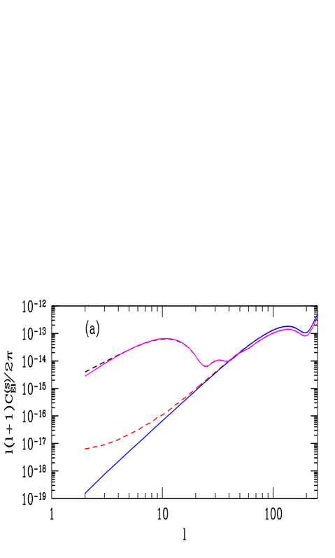
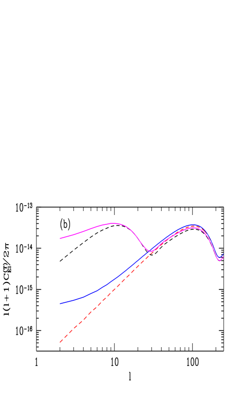
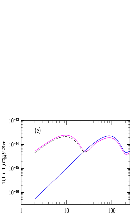
FIG. 1.: Comparison between exact calculation (solid lines) and small scale approximation (dashed lines) for standard CDM model with and without reionization. In the latter case we use optical depth of 0.2. The reionized models are the upper curves on large scales. The comparison is for scalar $E$ (a) and tensor $E$ (b) and $B$ (c) polarization power spectra. The spectra are in units of $T_{0}^{2}=(2.729K)^{2}$ and are normalized to COBE. While the predictions agree for large $l$ there are significant discrepancies in certain models for small $l$.

REFERENCES

[1] G. F. Smoot et al., Astrophys. J. Lett. 396, L1 (1992).
[2] D. Scott, J. Silk and
M. White, Science 268, 829 (1995);
J. R. Bond in “Cosmology and Large
Scale Structure”, ed R. Schaeffer et. al.,
Elsevier Science, Netherlands 1996.
[3] See the MAP homepage at
http://map.gsfc.nasa.gov.
[4] See the COBRAS/SAMBA homepage at
http://astro.estec.esa.nl/SA-general/Projects/Cobras/cobras.html
[5]
G. Jungman, M. Kamionkowski, A. Kosowsky,
and D. N. Spergel, Phys. Rev. Lett. 76, 1007 (1996);
Phys. Rev. D 54 1332 (1996).
[6] J. R. Bond et. al., Phys. Rev. Lett.
72, 13 (1994).
[7]
J. R. Bond and G. Efstathiou,
Mon. Not. R. Astr. Soc. 226, 655 (1987);
[8]
R. Crittenden, R. L. Davis, and P. J. Steinhardt,
Astrophys. J. Lett. 417, L13 (1993).
[9]
R. A. Frewin, A. G. Polnarev, and P. Coles, Mon. Not. R. Astron. Soc.
266, L21 (1994).
[10]
Coulson, D., Crittenden, R. G., & Turok, N. Phys. Rev. Lett. 73, 2390(1994).
[11]
R. G. Crittenden,
D. Coulson, and N. G. Turok, Phys. Rev. D 52, 5402 (1995).
[12]
M. Zaldarriaga and D. Harari, Phys. Rev. D 52, 3276 (1995).
[13] M. Zaldarriaga, Report no.
astro-ph/9608050, 1996 (unpublished).
[14] U. Seljak, Report no. astro-ph/9608131, 1996 (unpublished).
[15] U. Seljak, and M. Zaldarriaga, Report no.
astro-ph/9609169, 1996 (unpublished).
[16] M. Kamionkowski, A. Kosowsky and A. Stebbins,
Report no. astro-ph/9609132, 1996 (unpublished).
[17] A. Kosowsky, Ann. Phys. 246, 49 (1996).
[18] A. G. Polnarev, Sov. Astron. 29, 607 (1985).
[19]
J. N. Goldberg et al., J. Math. Phys. 8, 2155.
[20] E. Newman and R. Penrose, J. Math. Phys. 7,863 (1966).
[21] U. Seljak, and M. Zaldarriaga, Astrophys. J. 469,
437 (1996).
[22] S. Chandrasekhar, “Radiative Transfer”, Dover,
New York, 1960.
[23] N. Kaiser, Mon. Not. R. Astron. Soc. 202, 1169 (1983).
[24]
C. P. Ma and E. Bertschinger, Astrophys. J. 455, 7 (1995).
[25] L. F. Abbot and R. K. Schaeffer, Astrophys. J. 308
546, (1986).
[26] L. Knox,
Phys. Rev. D. 52, 4307 (1995).
[27] See http://cfata2.harvard.edu/uros/index.html
or http://arcturus.mit.edu/ matiasz/.
[28] K. S. Thorne, Rev. Mod. Phys. 52, 299.