[

Signature of Gravity Waves in Polarization of the Microwave Background

Abstract

Using spin-weighted decomposition of polarization in the Cosmic Microwave Background (CMB) we show that a particular combination of Stokes $Q$ and $U$ parameters vanishes for primordial fluctuations generated by scalar modes, but does not for those generated by primordial gravity waves. Because of this gravity wave detection is not limited by cosmic variance as in the case of temperature fluctuations. We present the exact expressions for various polarization power spectra, which are valid on any scale. Numerical evaluation in inflation-based models shows that the expected signal is of the order of 0.5 $\mu K$, which could be directly tested in future CMB experiments.

]

It is now well established that temperature anisotropies in CMB offer one of the best probes of early universe, which could potentially lead to a precise determination of a large number of cosmological parameters [1, 2]. The main advantage of CMB versus more local probes of large-scale structure is that the fluctuations were created at an epoch when the universe was still in a linear regime. While this fact has long been emphasized for temperature anisotropies, the same holds also for polarization in CMB and as such it offers the same advantages as the temperature anisotropies in the determination of cosmological parameters. The main limitation of polarization is that it is predicted to be small: theoretical calculations show that CMB will be polarized at 5-10% level on small angular scales and much less than that on large angular scales [3, 4]. However, future CMB missions (MAP, Planck) will be so sensitive that even such low signals will be measurable. Even if polarization by itself cannot compete with the temperature anisotropies, a combination of the two could result in a much more accurate determination of certain cosmological parameters, in particular those that are limited by a finite number of multipoles in the sky (i.e. cosmic variance).

Primordial gravity waves produce fluctuations in the tensor component of the metric, which could result in a significant contribution to the CMB anisotropies on large angular scales. Unfortunately, the presence of scalar modes prevents one from clearly separating one contribution from another. If there are only a finite number of multipoles where tensor contribution is significant then there is a limit in amplitude beyond which tensors cannot be distingushed from random fluctuations. In a noise free experiment the tensor to scalar ratio $T/S$ needs to be larger than 0.15 to be measurable in temperature maps [5]. Independent determination of the tensor spectral slope $n_{T}$ is even less accurate and a rejection of the consistency relation in inflationary models $T/S=-7n_{T}$ is only possible if $|n_{T}|\gg(T/S)/7$ [5, 6]. Polarization produced by tensor modes has also been studied [7], but only in the small scale limit. In previous work correlations between Stokes parameters $Q$ and $U$ have been used. These two variables are not the most suitable for the analysis as they depend on the orientation of coordinate system. It was recently shown [4] that in Fourier space $Q$ and $U$ can be decomposed in two components, which do not depend on orientation. Moreover, scalar modes only contribute to one of the two, leaving the other as a probe of gravity waves. These arguments have been made in the small angle approximation. In this Letter we remove this limitation by presenting a full spherical analysis of polarization using Newman-Penrose spin-s spherical harmonic decomposition. An alternative decomposition in terms of tensor harmonics has been presented recently by [8]. We show that there is a particular combination of Stokes parameters that vanishes in the case of scalar modes, which can thus be used as a probe of gravity waves. We present the expression for the power spectrum of various polarization components using the integral solution [9] and evaluate it numerically for a variety of cosmological models. We also discuss the sensitivity needed to detect this signal and compare it to the expected sensitivities of future CMB satellites.

Linear polarization is a symmetric and traceless 2x2 tensor [10] that requires 2 parameters to fully describe it: $Q$ and $U$ Stokes parameters. These parameters depend on the orientation of the coordinate system on the sky. It is convenient to use $Q+iU$ and $Q-iU$ as the two independent combinations, which transform under right-handed rotation by an angle $\phi$ as $(Q+iU)^{\prime}=e^{-2i\phi}(Q+iU)$ and $(Q-iU)^{\prime}=e^{2i\phi}(Q-iU)$. These two quantities therefore have spin-weights $2$ and $-2$ respectively and can be decomposed into spin $\pm 2$ spherical harmonics ${}_{\pm 2}Y_{lm}$ (for a discussion of spin-weighted harmonics see [11])

$$(Q+iU)(\hat{\mathchoice{{\hbox{\boldmath$\displaystyle n$}}}{{\hbox{\boldmath$\textstyle n$}}}{{\hbox{\boldmath$\scriptstyle n$}}}{{\hbox{\boldmath$\scriptscriptstyle n$}}}}) = \sum_{lm}a_{2,lm}{}_{2}Y_{lm}(\hat{\mathchoice{{\hbox{\boldmath$\displaystyle n$}}}{{\hbox{\boldmath$\textstyle n$}}}{{\hbox{\boldmath$\scriptstyle n$}}}{{\hbox{\boldmath$\scriptscriptstyle n$}}}})$$ (1)

$$(Q-iU)(\hat{\mathchoice{{\hbox{\boldmath$\displaystyle n$}}}{{\hbox{\boldmath$\textstyle n$}}}{{\hbox{\boldmath$\scriptstyle n$}}}{{\hbox{\boldmath$\scriptscriptstyle n$}}}}) = \sum_{lm}a_{-2,lm}{}_{-2}Y_{lm}(\hat{\mathchoice{{\hbox{\boldmath$\displaystyle n$}}}{{\hbox{\boldmath$\textstyle n$}}}{{\hbox{\boldmath$\scriptstyle n$}}}{{\hbox{\boldmath$\scriptscriptstyle n$}}}}).$$ (2)

Spin $s$ spherical harmonics form a complete orthonormal system for each value of $s$. An important property of spin-weighted basis is that there exists spin raising and lowering operators $\;\raise 1.5pt\hbox{${}^{\prime}$}\hskip-6.0pt\partial\;$ and $\;\overline{\raise 1.5pt\hbox{${}^{\prime}$}\hskip-6.0pt\partial}\;$ (see [11] for their explicit form). By acting twice with a spin lowering and raising operator on $(Q+iU)$ and $(Q-iU)$ respectively one obtains quantities of spin 0, which are rotationally invariant. These quantities can be treated like the temperature and no ambiguities connected with the orientation of coordinate system on the sky will arise. Conversely, by acting with spin lowering and raising operators on usual harmonics spin $s$ harmonics can be written explicitly in terms of derivatives of the usual spherical harmonics [11]. Their action on ${}_{\pm 2}Y_{lm}$ leads to

$$\;\overline{\raise 1.5pt\hbox{${}^{\prime}$}\hskip-6.0pt\partial}\;^{2}(Q+iU)(\hat{\mathchoice{{\hbox{\boldmath$\displaystyle n$}}}{{\hbox{\boldmath$\textstyle n$}}}{{\hbox{\boldmath$\scriptstyle n$}}}{{\hbox{\boldmath$\scriptscriptstyle n$}}}}) = \sum_{lm}\left({[l+2]!\over[l-2]!}\right)^{1/2}a_{2,lm}Y_{lm}(\hat{\mathchoice{{\hbox{\boldmath$\displaystyle n$}}}{{\hbox{\boldmath$\textstyle n$}}}{{\hbox{\boldmath$\scriptstyle n$}}}{{\hbox{\boldmath$\scriptscriptstyle n$}}}})$$ (3)

$$\;\raise 1.5pt\hbox{${}^{\prime}$}\hskip-6.0pt\partial\;^{2}(Q-iU)(\hat{\mathchoice{{\hbox{\boldmath$\displaystyle n$}}}{{\hbox{\boldmath$\textstyle n$}}}{{\hbox{\boldmath$\scriptstyle n$}}}{{\hbox{\boldmath$\scriptscriptstyle n$}}}}) = \sum_{lm}\left({[l+2]!\over[l-2]!}\right)^{1/2}a_{-2,lm}Y_{lm}(\hat{\mathchoice{{\hbox{\boldmath$\displaystyle n$}}}{{\hbox{\boldmath$\textstyle n$}}}{{\hbox{\boldmath$\scriptstyle n$}}}{{\hbox{\boldmath$\scriptscriptstyle n$}}}}).$$ (4)

With these definitions the expressions for the expansion coefficients of the two polarization variables become

$$a_{2,lm} = \left({[l-2]!\over[l+2]!}\right)^{1/2}\int d\Omega\;Y_{lm}^{*}(\hat{\mathchoice{{\hbox{\boldmath$\displaystyle n$}}}{{\hbox{\boldmath$\textstyle n$}}}{{\hbox{\boldmath$\scriptstyle n$}}}{{\hbox{\boldmath$\scriptscriptstyle n$}}}})\;\overline{\raise 1.5pt\hbox{${}^{\prime}$}\hskip-6.0pt\partial}\;^{2}(Q+iU)(\hat{\mathchoice{{\hbox{\boldmath$\displaystyle n$}}}{{\hbox{\boldmath$\textstyle n$}}}{{\hbox{\boldmath$\scriptstyle n$}}}{{\hbox{\boldmath$\scriptscriptstyle n$}}}})$$ (5)

$$a_{-2,lm} = \left({[l-2]!\over[l+2]!}\right)^{1/2}\int d\Omega\;Y_{lm}^{*}(\hat{\mathchoice{{\hbox{\boldmath$\displaystyle n$}}}{{\hbox{\boldmath$\textstyle n$}}}{{\hbox{\boldmath$\scriptstyle n$}}}{{\hbox{\boldmath$\scriptscriptstyle n$}}}})\;\raise 1.5pt\hbox{${}^{\prime}$}\hskip-6.0pt\partial\;^{2}(Q-iU)(\hat{\mathchoice{{\hbox{\boldmath$\displaystyle n$}}}{{\hbox{\boldmath$\textstyle n$}}}{{\hbox{\boldmath$\scriptstyle n$}}}{{\hbox{\boldmath$\scriptscriptstyle n$}}}}).$$ (6)

To obtain the expression for the polarization power spectrum we will use the integral solution of the Boltzmann equation [9]. In the case of scalar perturbations for any given Fourier mode $\textstyle k$ only $Q^{(S)}$ is generated in the frame where $\mathchoice{{\hbox{\boldmath$\displaystyle k$}}}{{\hbox{\boldmath$\textstyle k$}}}{{\hbox{\boldmath$\scriptstyle k$}}}{{\hbox{\boldmath$\scriptscriptstyle k$}}}\parallel\hat{\mathchoice{{\hbox{\boldmath$\displaystyle z$}}}{{\hbox{\boldmath$\textstyle z$}}}{{\hbox{\boldmath$\scriptstyle z$}}}{{\hbox{\boldmath$\scriptscriptstyle z$}}}}$ [12],

$$Q^{(S)}(\hat{\mathchoice{{\hbox{\boldmath$\displaystyle n$}}}{{\hbox{\boldmath$\textstyle n$}}}{{\hbox{\boldmath$\scriptstyle n$}}}{{\hbox{\boldmath$\scriptscriptstyle n$}}}},\mathchoice{{\hbox{\boldmath$\displaystyle k$}}}{{\hbox{\boldmath$\textstyle k$}}}{{\hbox{\boldmath$\scriptstyle k$}}}{{\hbox{\boldmath$\scriptscriptstyle k$}}}) = {3\over 4}(1-\mu^{2})\int d\tau e^{ix\mu}g(\tau)\Pi(k,\tau)$$ (7)

where $x=k(\tau_{0}-\tau)$ and $\tau$ is the conformal time with $\tau_{0}$ its present value. Directions in the sky are denoted with polar coordinates ($\theta$, $\phi$) and $\mu=\cos(\theta)$. We introduced the visibility function $g(\tau)=\dot{\kappa}e^{-\kappa}$, where $\dot{\kappa}$ is the differential optical depth for Thomson scattering, $\dot{\kappa}=an_{e}x_{e}\sigma_{T}$, $a(\tau)$ is the expansion factor normalized to unity today, $n_{e}$ is the electron density, $x_{e}$ is the ionization fraction and $\sigma_{T}$ is the Thomson cross section. The source term $\Pi=\Delta_{T2}^{(S)}+\Delta_{P2}^{(S)}+\Delta_{P0}^{(S)}$ was expressed in terms of temperature quadrupole $\Delta_{T2}^{(S)}$, polarization monopole $\Delta_{P0}^{(S)}$ and its quadrupole $\Delta_{P2}^{(S)}$. Because $U^{(S)}=0$ and $Q^{(S)}$ is only a function of $\mu$ in the $\mathchoice{{\hbox{\boldmath$\displaystyle k$}}}{{\hbox{\boldmath$\textstyle k$}}}{{\hbox{\boldmath$\scriptstyle k$}}}{{\hbox{\boldmath$\scriptscriptstyle k$}}}\parallel\hat{\mathchoice{{\hbox{\boldmath$\displaystyle z$}}}{{\hbox{\boldmath$\textstyle z$}}}{{\hbox{\boldmath$\scriptstyle z$}}}{{\hbox{\boldmath$\scriptscriptstyle z$}}}}$ frame it follows $\;\overline{\raise 1.5pt\hbox{${}^{\prime}$}\hskip-6.0pt\partial}\;^{2}(Q+iU)=\;\raise 1.5pt\hbox{${}^{\prime}$}\hskip-6.0pt\partial\;^{2}(Q-iU)$ and so $a^{(S)}_{2,lm}=a^{(S)}_{-2,lm}$. It is convenient to introduce two orthogonal combinations $a_{E,lm}=-(a_{2,lm}+a_{-2,lm})/2$ and $a_{B,lm}=(a_{2,lm}-a_{-2,lm})/2$. Here $E$ and $B$ refer to electric and magnetic type parities [13] and we have chosen the overall sign to agree with the small scale expressions in [4]. Note that our $E$ and $B$ are proportional to $G$ and $C$ in [8]. We find that $a_{B,lm}^{(S)}=0$ and only $a_{E,lm}^{(S)}$ is non-zero. The polarization power spectrum is defined as the rotationally invariant quantity $C_{l}={1\over 2l+1}\sum_{m}a_{lm}^{*}a_{lm}$. For $E$ its ensemble average can be obtained by acting twice with spin raising (or lowering) operator on equation 7 leading to (see [14] for details)

$$C_{El}^{(S)} = (3\pi)^{2}{(l+2)!\over(l-2)!}\int k^{2}dkP_{\phi}(k)$$ (8)

$$\times \left(\int d\tau g(\tau)\Pi(k,\tau){j_{l}(x)\over x^{2}}\right)^{2},$$ (9)

where $j_{l}(x)$ is the spherical Bessel function of order $l$ and $P_{\phi}(k)$ is the primordial power spectrum of scalar metric perturbations, usually assumed to be a power law $P_{\phi}(k)\propto k^{n-4}$.

In the case of tensors the form for $Q$ and $U$ in the frame where $\mathchoice{{\hbox{\boldmath$\displaystyle k$}}}{{\hbox{\boldmath$\textstyle k$}}}{{\hbox{\boldmath$\scriptstyle k$}}}{{\hbox{\boldmath$\scriptscriptstyle k$}}}\parallel\hat{\mathchoice{{\hbox{\boldmath$\displaystyle z$}}}{{\hbox{\boldmath$\textstyle z$}}}{{\hbox{\boldmath$\scriptstyle z$}}}{{\hbox{\boldmath$\scriptscriptstyle z$}}}}$ is [7]

$$Q(\hat{\mathchoice{{\hbox{\boldmath$\displaystyle n$}}}{{\hbox{\boldmath$\textstyle n$}}}{{\hbox{\boldmath$\scriptstyle n$}}}{{\hbox{\boldmath$\scriptscriptstyle n$}}}},\mathchoice{{\hbox{\boldmath$\displaystyle k$}}}{{\hbox{\boldmath$\textstyle k$}}}{{\hbox{\boldmath$\scriptstyle k$}}}{{\hbox{\boldmath$\scriptscriptstyle k$}}}) = -(1+\mu^{2})e^{2i\phi}\int d\tau e^{ix\mu}g\Psi(k,\tau)\;+\;c.c.$$ (10)

$$U(\hat{\mathchoice{{\hbox{\boldmath$\displaystyle n$}}}{{\hbox{\boldmath$\textstyle n$}}}{{\hbox{\boldmath$\scriptstyle n$}}}{{\hbox{\boldmath$\scriptscriptstyle n$}}}},\mathchoice{{\hbox{\boldmath$\displaystyle k$}}}{{\hbox{\boldmath$\textstyle k$}}}{{\hbox{\boldmath$\scriptstyle k$}}}{{\hbox{\boldmath$\scriptscriptstyle k$}}}) = -2i\mu e^{2i\phi}\int d\tau e^{ix\mu}g\Psi(k,\tau)\;+\;c.c.,$$ (11)

where the source is a complex sum over the two independent tensor polarization states, $\Psi=(\Psi^{+}-i\Psi^{\times})/2$, and can be expressed in terms of temperature and polarization multipoles as [7] $\Psi={1\over 10}\tilde{\Delta}_{T0}^{(T)}+{1\over 7}\tilde{\Delta}_{T2}^{(T)}+{3\over 70}\tilde{\Delta}_{T4}^{(T)}-{3\over 5}\tilde{\Delta}_{P0}^{(T)}+{6\over 7}\tilde{\Delta}_{P2}^{(T)}-{3\over 70}\tilde{\Delta}_{P4}^{(T)}$. This time $\;\overline{\raise 1.5pt\hbox{${}^{\prime}$}\hskip-6.0pt\partial}\;^{2}(Q+iU)$ and $\;\raise 1.5pt\hbox{${}^{\prime}$}\hskip-6.0pt\partial\;^{2}(Q-iU)$ are not equal, so both $a_{E,lm}^{(T)}$ and $a_{B,lm}^{(T)}$ will be nonzero. Using a similar procedure as above we obtain their power spectra [14]

$$C {}_{El}^{(T)}=(4\pi)^{2}\int k^{2}dkP_{h}(k)$$ (12)

$$\times \Big{|}\int d\tau g(\tau)\Psi(k,\tau)\Big{[}-j_{l}(x)+j_{l}^{\prime\prime}(x)+{2j_{l}(x)\over x^{2}}+{4j_{l}^{\prime}(x)\over x}\Big{]}\Big{|}^{2}$$ (13)

$$C {}_{Bl}^{(T)}=(4\pi)^{2}\int k^{2}dkP_{h}(k)$$ (14)

$$\times \Big{|}\int d\tau g(\tau)\Psi(k,\tau)\Big{[}2j_{l}^{\prime}(x)+{4j_{l}\over x}\Big{]}\Big{|}^{2},$$ (15)

where $P_{h}(k)\propto k^{n_{T}-3}$ is the primordial power spectrum of gravity waves. In the small scale limit these expressions agree with those derived previously [4, 7].

Using the above expressions we may numerically evaluate the power spectra in various theoretical models. We use $T/S$ as the parameter determining the amplitude of tensor polarization. Fig. 1 shows the predictions for scalar and tensor contribution in standard CDM model with no reionization (a) and in reionized universe with optical depth of $\kappa=0.2$ (b). The latter value is typical in standard cosmological models [15]. We assumed $T/S=1$ and $n_{T}=(n_{s}-1)=-0.15$. In the no-reionization case both tensor spectra peak around $l\sim 100$ and give comparable contributions, although the $B$ channel is somewhat smaller. Comparing the scalar and tensor $E$ channels one can see that scalar polarization dominates for $T/S\raise 2.9pt\hbox{$\scriptstyle<$}\lower 0.5pt\hbox{$\scriptscriptstyle\sim$}\;1$. Even though tensor contribution is larger than scalar at low $l$, the overall power there is too small to be measurable. Tensor reconstruction in the $E$ channel suffers from similar drawbacks as in the case of temperature anisotropies: because of large scalar contribution cosmic variance prevents one to isolate very small tensor contributions [5]. The situation improves if the epoch of reionization occured sufficiently early that a moderate optical depth to Thomson scattering is accumulated (Fig. 1b). In this case there is an additional peak at low $l$ [16] and the relative contribution of tensor to scalar polarization in $E$ channel around $l=10$ is higher than around $l=100$. Still, if $T/S\ll 1$ cosmic variance again limits one to extract unambiguously the tensor contribution. It is in this limit that the importance of $B$ channel becomes crucial. This channel is not contaminated by scalar contribution and is only limited by noise, so in principle with sufficient noise sensitivity one can detect even very small tensor to scalar ratios. Moreover, a detection of signal in this channel would be a model independent detection of non-scalar perturbations. In the following we will discuss sensitivity to gravity waves using both only $B$ channel information and all available information.

We can obtain an estimate of how well can tensor parameters be reconstructed by using only the $B$ channel and assuming that the rest of cosmological parameters will be accurately determined from the temperature and $E$ polarization measurements. While this test might not be the most powerful it is the least model dependent: any detection in $B$ channel would imply a presence of non-scalar fluctuations and therefore give a significant constraint on cosmological models. Because the $B$ channel does not cross-correlate with either $T$ or $E$ [4, 8, 14] only its auto-correlation needs to be considered. A useful method to estimate parameter sensitivity for a given experiment is to use the Fisher information matrix [1, 4, 8, 14]

$$\alpha_{ij} = \sum_{l=2}^{l_{\rm max}}{(2l+1)f_{\rm sky}\over 2}$$ (16)

$$\times \Big{[}C_{Bl}+{4\pi\sigma^{2}\over N}e^{l(l+1)\sigma_{b}^{2}}\Big{]}^{-2}\left({\partial C_{Bl}\over\partial s_{i}}\right)\left({\partial C_{Bl}\over\partial s_{j}}\right),$$ (17)

where $f_{\rm sky}$ is the sky coverage. Receiver noise can be parametrized by $4\pi\sigma^{2}/N$, where $\sigma$ is the noise per pixel and $N$ is the number of pixels. Typical values are $(0.15\mu{\rm K})^{2}$ for MAP and $(0.025\mu{\rm K})^{2}$ for the most sensitive Planck bolometer channel in one year of observation. In our case the parameters $s_{i}$ can be $T/S$ and $n_{T}$, so that the matrix is only 2x2. The error on each parameter is given by $(\alpha^{-1}_{ii})^{1/2}$ if the other parameter is assumed to be unknown and $(\alpha_{ii})^{-1/2}$ if the other parameter is assumed to be known. Using this expression we may calculate the experiment sensitivity to these parameters. Current inflationary models and limits from large scale structure and COBE predict $T/S$ to be less than unity. Figure 1 shows that the expected amplitude in this case is below 0.5$\mu$K. We find that MAP is not sufficiently sensitive in $B$ channel to detect these low levels. On the other hand, Planck will be much more sensitive and can detect $T/S>0.3$ if tensor index $n_{T}$ is assumed to be known (for example through the consistency relation). For the underlying model with $T/S=1$ one can determine it with an error $\Delta(T/S)\sim 0.1$. If tensor index is not known then a combination of the two parameters, which corresponds to the total power under the $B$ curve in figure 1, can still be determined with the same accuracy.

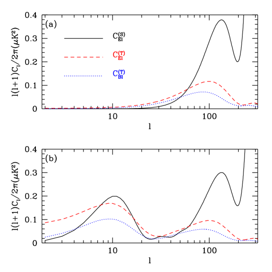
FIG. 1.: Multipole moments for the three polarization spectra for no-reionization case (a) and reionized case with optical depth of 0.2 (b). The underlying model is “standard CDM” with $T/S=1$.

Separate determination of the tensor amplitude and slope from the $B$ channel is only possible in reionized models. In the no-reionization model the contribution to $B$ is very narrow in $l$ space and the leverage on $n_{T}$ independent of $T/S$ is small, so that the correlation coefficient $\alpha_{12}/(\alpha_{11}\alpha_{22})^{1/2}$ is almost always close to unity. A modest amount of reionization improves the separation; in the reionized models the power spectrum for $B$ is bimodal (figure 1) and the overall signal is higher, which gives a better leverage on $n_{T}$ independent of $T/S$. For $\kappa=0.2$ the Planck errors are $\Delta(T/S)\sim 0.15$ and $\Delta n_{T}\sim 0.1$ for the underlying model with $T/S=1$. These results depend on the overall amplitude relative to the noise level. As long as both peaks can be separated from the noise one can determine the tensor slope, which allows to test the inflationary consistency relation.

Combining all the information by adding temperature, $E$ polarization and their cross-correlation further improves these estimates. In this case other parameters that affect scalar modes such as baryon density, Hubble constant or cosmological constant enter as well and the results become more model dependent [2]. Fisher information matrix has to be generalized to include all the parameters that can be degenerate with the tensor parameters. The results depend on the class of models and number of parameters one restricts to in the analysis, as opposed to the results based on $B$ channel above, which depend only on the two main parameters that characterize the gravity wave production. As a typical example, for $T/S=0.1$ and $\kappa=0.1$ one can determine $\Delta(T/S)=0.05$ and $\Delta n_{T}=0.2$ with Planck [2]. These errors improve further if a model with higher $T/S$ or $\kappa$ is assumed. For the same underlying model without using polarization the expected errors are $\Delta T/S\sim 0.26$ and $\Delta n_{T}\sim 1$, significantly worse than with polarization. Even for MAP the limits on $T/S$ improve by a factor of 2 when polarization information is included.

To summarize the above discussion, future CMB missions are likely to reach the sensitivities needed to measure (or reject) a significant production of primordial gravity waves in the early universe through polarization measurements, which will vastly improve the limits from temperature measurements only and allow a test of consistency relation. The more challenging question is the foreground subtraction at the required level. At low frequencies radio point sources and synchrotron emission from our galaxy dominate the foregrounds and both are polarized at a 10% level. Their contribution decreases at higher frequencies and with several frequency measurements one can subtract these foregrounds at frequencies around 100 GHz at the required microkelvin level. At even higher frequencies dust is the dominant foreground, but is measured to be only a few percent polarized [17]. We hope that the signature of gravity waves discussed here would provide further motivation to pursue the feasibility studies of polarization measurements.

While we only discussed scalar and tensor modes, vector modes, if present before recombination, will also contribute to both polarization channels and so could contaminate the signature of gravity waves. At present there are no viable cosmological models that would produce a significant contribution of vector modes without a comparable amount of tensor modes. In inflationary models vector modes, even if produced during inflation, decay away and are not significant during recombination. In topological defect models nonlinear sources continuously create both vector and tensor modes and so some of the signal in $B$ channel could be caused by vector modes. Even in these models however some fraction of signal in $B$ will still be generated by tensor modes and in any case, absence of signal in $B$ channel would rule out such models. Polarization thus offers a unique way to probe cosmological models that is within reach of the next generation of CMB experiments.

REFERENCES

- [1] G. Jungman, M. Kamionkowski, A. Kosowsky, and D. N. Spergel, Phys. Rev. Lett. 76, 1007 (1996); ibid Phys. Rev. D 54 1332 (1996).
- [2] M. Zaldarriaga, D. N. Spergel and U. Seljak, in preparation.
- [3] M. Rees, Astrophys. J. 153, L1 (1968); J. R. Bond and G. Efstathiou, Astrophys. J. 285, L47 (1984); ibid Mon. Not. R. Astr. Soc. 226, 655 (1987); M. Zaldarriaga and D. Harari, Phys. Rev. D 52, 3276 (1995).
- [4] U. Seljak, Report no. astro-ph/9608131, 1996 (unpublished).
- [5] L. Knox, and M. S. Turner, Phys. Rev. Lett. 73, 3347 (1996).
- [6] S. Dodelson, L. Knox, and E. W. Kolb, Phys. Rev. Lett. 72, 3443 (1994).
- [7] A. G. Polnarev, Sov. Astron. 29, 607 (1985); R. Crittenden, R. L. Davis, and P. J. Steinhardt, Astrophys. J. Lett. 417, L13 (1993); R. A. Frewin, A. G. Polnarev, and P. Coles, Mon. Not. R. Astron. Soc. 266, L21 (1994); R. G. Crittenden, D. Coulson, and N. G. Turok, Phys. Rev. D 52, 5402 (1995); A. Kosowsky, Ann. Phys. 246, 49 (1996).
- [8] M. Kamionkowski, A. Kosowsky and A. Stebbins, Report no. astro-ph/9609132, ibid astro-ph/9611125, 1996 (unpublished).
- [9] U. Seljak, and M. Zaldarriaga, Astrophys. J. 469, 437 (1996).
- [10] Circular polarization cannot be generated in the early universe through the process of Thomson scattering, so Stokes parameter is 0.
- [11] J. N. Goldberg et al., J. Math. Phys. 8, 2155(1966).
- [12] N. Kaiser, Mon. Not. R. Astron. Soc. 202, 1169 (1983).
- [13] E. Newman, and R. Penrose, J. Math. Phys. 7, 863 (1966).
- [14] M. Zaldarriaga, and U. Seljak, Phys. Rev. D 55, 1830 (1997).
- [15] Z. Haiman, and A. Loeb, astro-ph/9611028, 1996 (unpublished).
- [16] M. Zaldarriaga, Phys. Rev. D 55, 1822 (1997).
- [17] R. G. Hildebrand, and M. Dragovan, Astrophys. J. 450, 663 (1995).