Abstract

I discuss two cosmological tests to determine the cosmological density parameter $\Omega_{0}$ the cosmological constant $\lambda_{0}$, which make use of the anisotropy of the two-point correlation functions due to the peculiar velocity field and the cosmological redshift-space distortion.

I Introduction

The three-dimensional distribution of galaxies in the redshift surveys differ from the true one since the distance to each galaxy cannot be determined by its redshift $z$ only; for $z\ll 1$ the peculiar velocity of galaxies, typically $\sim(100-1000){\rm km/sec}$, contaminates the true recession velocity of the Hubble flow, while the true distance for objects at $z\lower 2.15277pt\hbox{$\;\buildrel>\over{\sim}\;$}1$ sensitively depends on the (unknown and thus assumed) cosmological parameters. This hampers the effort to understand the true distribution of large-scale structure of the universe. Nevertheless such redshift-space distortion effects are quite useful since through the detailed theoretical modelling, one can derive the peculiar velocity dispersions of galaxies as a function of separation, and also can infer the cosmological density parameter $\Omega_{0}$ and the dimensionless cosmological constant $\lambda_{0}$, for instance. In what follows, I will present two specific topics concerning the redshift distortion; the small-scale pair-wise peculiar velocity dispersions of galaxies[2], and anisotropies in the two-point correlation functions[3] at high redshifts.

II $\Omega_{0}$ from nonlinear galaxy clustering

Assuming that particle pairs in expanding universes are in “statistical equilibrium” on small scales, their relative peculiar velocity dispersion can be computed as a function of their separation. The result is called the cosmic virial theorem [4, 5] (CVT, hereafter) which predicts the one-dimensional pair-wise relative peculiar velocity dispersion $\sigma_{{\scriptscriptstyle{1D}},{\scriptscriptstyle{CVT}}}$ as a function of $\Omega_{0}$.

The observed two- and three-point correlation functions of galaxies, $\xi_{\rm g}$ and $\zeta_{\rm g}$, are well approximated by the simple form[6, 7]:

$$\xi_{\rm g}(r)=\left({r_{\scriptscriptstyle{0}}\over r}\right)^{\gamma},\qquad\zeta_{\rm g}(r_{1},r_{2},r_{3})=Q_{\rm g}\,[\xi_{\rm g}(r_{1})\xi_{\rm g}(r_{2})+\xi_{\rm g}(r_{2})\xi_{\rm g}(r_{3})+\xi_{\rm g}(r_{3})\xi_{\rm g}(r_{1})]$$ (1)

where $r_{0}=(5.4\pm 0.3){\hbox{$h^{-1}$}{\rm Mpc}}$, $\gamma=1.77\pm 0.04$, $Q_{\rm g}=1.29\pm 0.21$. Thus it is reasonable to assume that the two- and three-point correlation functions of mass, $\xi_{\rho}$ and $\zeta_{\rho}$, also obey the same scaling except for the overall amplitude:

$$\xi_{\rho}(r)={1\over b_{\rm g}^{2}}\xi_{\rm g}(r),\qquad\zeta_{\rho}(r_{1},r_{2},r_{3})={Q_{\rho}\over Q_{\rm g}b_{\rm g}^{4}}\zeta_{\rm g}(r_{1},r_{2},r_{3}).$$ (2)

Then the CVT prediction of the small-scale peculiar velocity dispersion is given by[2, 4]

$$\sigma_{{\scriptscriptstyle{1D}},{\scriptscriptstyle{CVT}}}(r)=1460\sqrt{\Omega_{0}Q_{\rho}\over 1.3b_{\rm g}^{2}}\sqrt{I(\gamma)\over 33.2}5.4^{\frac{\gamma-1.8}{2}}\left({r_{\scriptscriptstyle{0}}\over 5.4{\hbox{$h^{-1}$}{\rm Mpc}}}\right)^{\frac{\gamma}{2}}\left({r\over 1{\hbox{$h^{-1}$}{\rm Mpc}}}\right)^{\frac{2-\gamma}{2}}{\rm km/sec},$$ (3)

$$I(\gamma)\equiv{\pi\over(\gamma-1)(2-\gamma)(4-\gamma)}$$ (4)

$$~{}~{}~{}~{}\times\int_{0}^{\infty}\,dx\,{1+x^{-\gamma}\over x^{2}}\left\{(1+x)^{4-\gamma}-|1+x|^{4-\gamma}-(4-\gamma)x\left[(1+x)^{2-\gamma}+|1+x|^{2-\gamma}\right]\right\},$$ (5)

and numerically $I(1.65)\sim 25.4$, $I(1.8)\sim 33.2$, and $I(1.95)\sim 55.6$.

To what extent is the CVT prediction reliable ? In order to examine this, I compared $\sigma_{{\scriptscriptstyle{1D}},{\scriptscriptstyle{CVT}}}(r)$ with the one-dimensional peculiar velocity dispersions of particle pairs with separation $r=|{\mbox{\boldmath$r$}}_{1}-{\mbox{\boldmath$r$}}_{2}|$ directly computed from N-body simulations for cold dark matter models: $v_{12{\scriptscriptstyle\|}}(r)\equiv\langle[({\mbox{\boldmath$v$}}_{1}-{\mbox{\boldmath$v$}}_{2})\cdot({\mbox{\boldmath$r$}}_{1}-{\mbox{\boldmath$r$}}_{2})/|{\mbox{\boldmath$r$}}_{1}-{\mbox{\boldmath$r$}}_{2}|]^{2}\rangle^{1/2}$. Figure 1 summarizes the comparison which implies that $\sigma_{{\scriptscriptstyle{1D}},{\scriptscriptstyle{CVT}}}(r)$ reproduces the simulation result excellently for $0.1{\hbox{$h^{-1}$}{\rm Mpc}}\lower 2.15277pt\hbox{$\;\buildrel<\over{\sim}\;$}r\lower 2.15277pt\hbox{$\;\buildrel<\over{\sim}\;$}1{\hbox{$h^{-1}$}{\rm Mpc}}$; CVT is quite reliable in predicting $v_{12{\scriptscriptstyle\|}}(r)$ for $r<1{\hbox{$h^{-1}$}{\rm Mpc}}$. It should be stressed that the crucial assumption in deriving the prediction (3) is equation (2), and the result is independent of the theoretical model for dark matter. In this sense the prediction (3) is general, and the good agreement in CDM models should be ascribed to the fact that the CDM models actually satisfy the relation (3).

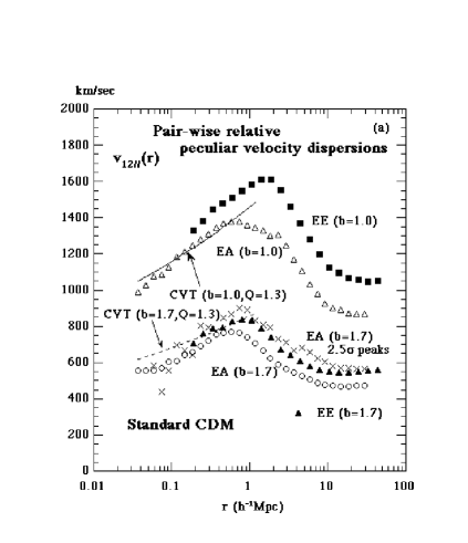
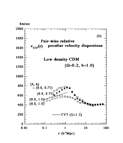
FIG. 1.: Pairwise relative peculiar velocity dispersions: comparison between predictions of the CVT and simulations (Suto 1993). (a) Standard CDM ($\Omega_{0}=1$, $\lambda_{0}=0$, $h=0.5$): Model EA employs $N=128^{3}$ particles in comoving $(130{\hbox{$h^{-1}$}{\rm Mpc}})^{3}$ box, while model EE employs $N=128^{3}$ particles in comoving $(200{\hbox{$h^{-1}$}{\rm Mpc}})^{3}$ box. The different symbols denote the results at different epochs for the models; EE at $b_{\rm g}=1$ (filled squares), EA at $b_{\rm g}=1$ (open triangles), EE at $b_{\rm g}=1.7$ (filled triangles), EA at $b_{\rm g}=1.7$ (open circles), and EA at $b_{\rm g}=1.7$ but for $2.5\sigma$ peak particles (crosses). The solid and dashed lines show the CVT prediction $\sigma_{{\scriptscriptstyle{1D}},{\scriptscriptstyle{CVT}}}(r)$ for $b_{\rm g}=1.0$ and $1.7$, respectively ($Q_{\rho}=1.3$). (b) Low-density CDM ($\Omega_{0}=0.2$, $b=1.0$): $(\lambda_{0},h)=(0,0.75)$ model with $N=128^{3}$ particles in comoving $(300{\hbox{$h^{-1}$}{\rm Mpc}})^{3}$ box (open squares), $(0.8,0.75)$ model with $N=128^{3}$ particles in comoving $(300{\hbox{$h^{-1}$}{\rm Mpc}})^{3}$ box (filled triangle), $(0.0,1.0)$ model with $64^{3}$ particles in comoving $(100{\hbox{$h^{-1}$}{\rm Mpc}})^{3}$ box (crosses), and $(0.8,1.0)$ model with $N=64^{3}$ particles in comoving $(100{\hbox{$h^{-1}$}{\rm Mpc}})^{3}$ box (open circles).

Using the anisotropy of the two-point correlation function of the CfA1 galaxy redshift survey, Davis and Peebles[7] estimated the line of sight peculiar velocity dispersions $\sigma_{\rm g,obs}^{2}(r_{p})$ of galaxy pairs seen projected at separation $r_{p}$. This is related to the dispersions $\langle v^{2}_{{\scriptscriptstyle{3D}},21}(r)\rangle$ for galaxy pairs with separation $r$ in three dimension as

$$\sigma_{\rm g,obs}^{2}(r_{p})={\displaystyle\int_{0}^{\infty}dy\,\xi_{\rm g}\left(\sqrt{r_{p}^{2}+y^{2}}\right)\,\left\langle v^{2}_{{\scriptscriptstyle{3D}},21}\left(\sqrt{r_{p}^{2}+y^{2}}\right)\right\rangle\over\displaystyle 3\int_{0}^{\infty}dy\,\xi_{\rm g}\left(\sqrt{r_{p}^{2}+y^{2}}\right)}.$$ (6)

Note that Davis and Peebles[7] found that $\sigma_{\rm g,obs}^{2}(r_{p})\propto r_{p}^{0.13\pm 0.04}$ which justifies our assumption of the mass correlation function $\xi(r)\propto r^{-1.8}$ as $\xi_{\rm g}(r)$ from a dynamical point of view. If $\xi(r)\propto r^{-\gamma}$ and $\langle v^{2}_{{\scriptscriptstyle{3D}},21}(r)\rangle\propto r^{2-\gamma}$, the corresponding CVT estimator corrected for the projection becomes

$$\sigma_{{\scriptscriptstyle{1D}},{\scriptscriptstyle{CVT}},proj}(r_{p})=C(\gamma)\,\sigma_{{\scriptscriptstyle{1D}},{\scriptscriptstyle{CVT}}}(r_{p})\qquad C(\gamma)\equiv\sqrt{\Gamma(\gamma/2)\,\Gamma(\gamma-3/2)\over\Gamma(\gamma/2-1/2)\,\Gamma(\gamma-1)},$$ (7)

where $\Gamma(x)$ is the Gamma function. Thus $C(\gamma)$ is the correction factor for the projection effect[2, 7]; $C(1.65)\sim 1.36$, $C(1.8)\sim 1.11$, $C(1.95)\sim 1.02$.

Independent estimates of $\sigma_{\rm g,obs}(r_{p})$ are available from several galaxy redshift catalogues[7, 11, 12, 13, 14, 15, 16]. As pointed out earlier by Mo, Jing, and Börner[13], the currently available redshift catalogues are far from the fair sample, and the observational estimate of $\sigma_{\rm g,obs}^{2}(r_{p})$ may differ from its true cosmic average due to the limited survey volume and the selection effect. Therefore it is meaningful to re-examine the problem in more details.

If the hierarchical relation (2) holds as is indicated from the galaxy distribution, the amplitudes of the two- and three-point correlation functions, or equivalently $b_{\rm g}$ and $Q_{\rho}$, are the two uncertain parameters in the CVT prediction (3). Recent numerical and analytical studies in nonlinear gravitational clustering seem to indicate that $Q_{\rho}$ can be approximated as a constant in the range of $0.5$ and $2$ which depends very weakly on the underlying cosmological model. Thus if the value of $b_{\rm g}$ is fixed from the COBE data assuming CDM models, for example, the CVT prediction (3) is completely specified.

Figure 2 plots the empirical fit for the COBE normalized $\sigma(8{\hbox{$h^{-1}$}{\rm Mpc}})$ and $b(8{\hbox{$h^{-1}$}{\rm Mpc}})\equiv 1/\sigma(8{\hbox{$h^{-1}$}{\rm Mpc}})$ by Nakamura[17] to the numerical computation by Sugiyama[18]. There I adopt the baryon density parameter $\Omega_{b}=0.015h^{-2}$. Incidentally it is amusing to note that $\Omega_{0}=0.2$, $\lambda_{0}=0.8$, and $h=0.7$ CDM model just corresponds to $b_{\rm g}=1$, i.e., galaxies faithfully trace mass in this model according to the COBE normalization.

Once the $b_{\rm g}$ is specified, it is easy to compute the CVT prediction (3). Figure 3 plots $\sigma_{{\scriptscriptstyle{1D}},{\scriptscriptstyle{CVT}},proj}(r=1{\hbox{$h^{-1}$}{\rm Mpc}})$ (eq.[7]) as a function of $\Omega_{0}$. The symbols denote several recent observational estimates which are shifted along the x-axis just for illustration. The left panel shows the dependence on $Q_{\rho}$ and the right panel shows how the CVT prediction is sensitive to their local value, or sample-to-sample variation of the data.

FIG. 2.: CDM spectrum normalization factor from COBE 2 year data. (a) top-hat mass rms fluctuation, $\sigma(8{\hbox{$h^{-1}$}{\rm Mpc}})$; (b) the biasing factor $b(8{\hbox{$h^{-1}$}{\rm Mpc}})\equiv 1/\sigma(8{\hbox{$h^{-1}$}{\rm Mpc}})$ in $\lambda_{0}=1-\Omega_{0}$ (solid curve) and $\lambda_{0}=0$ (dashed curve) CDM models ($h=0.7$ is assumed).

FIG. 3.: Pairwise relative peculiar velocity dispersions at $1{\hbox{$h^{-1}$}{\rm Mpc}}$ from the observations (symbols) compared with the predictions of the cosmic virial theorem in $\lambda_{0}=1-\Omega_{0}$ (thick curves) and $\lambda_{0}=0$ (thin curves) CDM models.

Figure 3 exhibits that both observational estimates and CVT predictions of $\sigma_{{\scriptscriptstyle{1D}}}(r=1{\hbox{$h^{-1}$}{\rm Mpc}})$ vary by a factor of $2\sim 3$ depending on the local clustering degree of each sample. Even allowing for these, however, it looks unlikely that high-density CDM models ($\Omega_{0}\lower 2.15277pt\hbox{$\;\buildrel>\over{\sim}\;$}0.5$) are compatible with the currently observed values of $\sigma_{{\scriptscriptstyle{1D}}}(r=1{\hbox{$h^{-1}$}{\rm Mpc}})$. In a similar argument, one may obtain strong upper limits on $\Omega_{0}$ in general cosmological scenarios as long as $b_{\rm g}$ is not much greater than unity.

III $\Omega_{0}$ and $\lambda_{0}$ from quasar clustering at high redshifts

As shown in the previous section, small-scale velocity dispersions of galaxies place strong upper limits on $\Omega_{0}$, fairly independently of $\lambda_{0}$. In turn, detailed analysis of clustering of objects at high redshifts will place a potentially important constraint on $\lambda_{0}$ via an effect which we call the cosmological redshift distortion[3]. A very similar idea was put forward independently by Ballinger, Peacock and Heavens[20] although they work entirely in k-space. The result that I describe below considers the analysis of two-point correlation functions, which would be more straightforward to derived from the quasar catalogues.

Let us consider a pair of objects located at redshifts $z_{1}$ and $z_{2}$ whose redshift difference $\delta z\equiv z_{1}-z_{2}$ is much less than the mean redshift $z\equiv(z_{1}+z_{2})/2$. Then the observable separations of the pair parallel and perpendicular to the line-of-sight direction, $s_{{\scriptscriptstyle\|}}$ and $s_{\bot}$, are given as $\delta z/H_{0}$ and $z\delta\theta/H_{0}$, respectively, where $H_{0}$ is the Hubble constant and $\delta\theta$ denotes the angular separation of the pair on the sky. The cosmological redshift-space distortion originates from the anisotropic mapping between the redshift-space coordinates, $(s_{\scriptscriptstyle\|},s_{\bot})$, and the real comoving ones[3], $(x_{\scriptscriptstyle\|},x_{\bot})\equiv(c_{\scriptscriptstyle\|}s_{\scriptscriptstyle\|},c_{\bot}s_{\bot})$; $c_{\bot}$ is written in terms of the angular diameter distance $D_{\scriptscriptstyle{A}}$ as $c_{\bot}=H_{0}(1+z)D_{\scriptscriptstyle{A}}/z$, and

$$c_{\scriptscriptstyle\|}(z)={H_{0}\over H(z)}={1\over\sqrt{\Omega_{0}(1+z)^{3}+(1-\Omega_{0}-\lambda_{0})(1+z)^{2}+\lambda_{0}}}.$$ (8)

The relation between the two-point correlation functions of quasars in redshift space, $\xi^{(s)}(s_{\bot},s_{\scriptscriptstyle\|})$, and that of mass in real space $\xi^{(r)}(x)$ can be derived in linear theory[27, 3]:

$$\xi^{(s)}(s_{\bot},s_{\scriptscriptstyle\|})=\left(1+{2\over 3}\beta(z)+{1\over 5}[\beta(z)]^{2}\right)\xi_{0}(x)P_{0}(\mu)-\left({4\over 3}\beta(z)+{4\over 7}[\beta(z)]^{2}\right)\xi_{2}(x)P_{2}(\mu)$$ (9)

$$\qquad\qquad+\frac{8}{35}[\beta(z)]^{2}\xi_{4}(x)P_{4}(\mu),$$ (10)

where $x\equiv\sqrt{{c_{\scriptscriptstyle\|}}^{2}{s_{\scriptscriptstyle\|}}^{2}+{c_{\bot}}^{2}{s_{\bot}}^{2}}$, $\mu\equiv c_{{\scriptscriptstyle\|}}s_{{\scriptscriptstyle\|}}/x$, $P_{n}$’s are the Legendre polynomials,

$$\beta(z)\equiv{1\over b(z)}\frac{d\ln D(z)}{d\ln a},\qquad\xi_{2l}(x)={(-1)^{l}\over x^{2l+1}}\left(\int_{0}^{x}xdx\right)^{l}x^{2l}\left({d\over dx}{1\over x}\right)^{l}x\xi^{(r)}(x),$$ (11)

and $D(z)$ is the linear growth rate.

For specific examples, we compute $\xi^{(s)}(s_{\bot},s_{{\scriptscriptstyle\|}})$ in linear theory applying equations (9) and (11) in CDM models with $H_{0}=70$ km$\cdot$s${}^{-1}\cdot$Mpc^-1[19]. The resulting contours are plotted in Figure 4. The four sets of values of $\Omega_{0}$ and $\lambda_{0}$ are indicated at the top of each panel. We adopt the COBE normalization[17, 18, 28].

FIG. 4.: The contours of $\xi^{(s)}(s_{\bot},s_{{\scriptscriptstyle\|}})$ in CDM models at $z=0$ (upper panels) and $z=3$ (lower panels). Solid and dashed lines indicate the positive and negative $\xi^{(s)}$, respectively. Contour spacings are $\Delta{\rm log}_{10}|\xi|=0.25$.

In order to quantify the cosmological redshift distortion in Figure 4, let us introduce the anisotropy parameter $\xi^{(s)}_{{\scriptscriptstyle\|}}(s)/\xi^{(s)}_{\bot}(s)$, where $\xi^{(s)}_{\bot}(s)\equiv\xi^{(s)}(s,0)$ and $\xi^{(s)}_{{\scriptscriptstyle\|}}(s)\equiv\xi^{(s)}(0,s)$. The left four panels in Figure 5 show the anisotropy parameter against $z$ in CDM models. This clearly exhibits the extent to which one can discriminate the different $\lambda_{0}$ models on the basis of the anisotropies in $\xi^{(s)}$ at high redshifts.

FIG. 5.: The anisotropy parameter $\xi^{(s)}_{{\scriptscriptstyle\|}}(s)/\xi^{(s)}_{\bot}(s)$ as a function of $z$. Upper and lower panels assume that $b=1$ and $2$, respectively. From left to right, the panel corresponds to CDM at $s=10{\hbox{$h^{-1}$}{\rm Mpc}}$, CDM at $s=20{\hbox{$h^{-1}$}{\rm Mpc}}$, a power-law model with $\gamma=1.8$ and a power-law model with $\gamma=1.0$.

IV Conclusions

One can roughly divide the source of cosmological information into four regimes; (i) linear regime ($r\lower 2.15277pt\hbox{$\;\buildrel>\over{\sim}\;$}10{\hbox{$h^{-1}$}{\rm Mpc}}$) at $z\sim 0$, (ii) nonlinear regime ($r\sim 1{\hbox{$h^{-1}$}{\rm Mpc}}$) at $z\sim 0$, (iii) linear regime at $z\gg 1$, and (iv) nonlinear regime at $z\gg 1$.

The clustering feature at $z\sim 0$ is best probed by galaxy redshift surveys, and the current samples, albeit statistically limited by the number of galaxies, are heavily used for a variety of cosmological tests. The conventional redshift-space distortion analysis[26, 27] in the regime (i) yields generally $\Omega_{0}\ll 1$; $\Omega_{0}^{0.6}/b_{\rm g}(z=0)=0.55\pm 0.12$ for instance from the Durham/UKST galaxy redshift survey of $\sim 2500$ galaxies. I have shown in the first part of the talk that the small-scale peculiar velocity dispersions of galaxies in comparison withe the CVT prediction constrains the value of $\sqrt{\Omega_{0}Q_{\rho}}/b_{\rm g}(z=0)$. Allowing for the sample-to-sample variation of the available redshift surveys and the uncertainties for $Q_{\rho}$ and $b_{\rm g}(z=0)$, I still conclude that the observation in the regime (ii) favors low-density universes $\Omega_{0}\lower 2.15277pt\hbox{$\;\buildrel<\over{\sim}\;$}0.5$ at most.

In contrast to the regimes (i) and (ii), the proper analysis of the regimes (iii) and (iv) requires a large number of quasars homogeneously samples which are not currently available. Therefore the cosmological tests in theses regimes have not been fully explored even theoretically. In the second part of the talk, I presented an example in this line of investigations, cosmological redshift-space distortion[3]. I derived the formula which describes the degree of the anisotropies of two-point correlation functions of quasars in linear regime (iii), and argued that it is a potentially powerful discriminator of $\lambda_{0}$ once $\Omega_{0}$ is determined from the nearby observation. From the observational point of view, however, it would be much easier to detect the the anisotropies of two-point correlation functions in the regime (iv). We are currently approaching this important area of research using the nonlinear theory and simulations[30, 31].

I do look forward to the next-generation redshift surveys which will definitely provide data catalogues and thus make feasible these precise cosmological tests.

REFERENCES

• [1]
• [2] Y. Suto, Prog.Theor.Phys. 90, 1173 (1993).
• [3] T. Matsubara and Y. Suto, Astrophys.J. (Letters), October 10 issue, in press (1996).
• [4] P.J.E. Peebles, Astrophys.Sp.Sci.,45,3 (1976).
• [5] P.J.E. Peebles,The Large Scale Structure of the Universe, Princeton University Press (1980).
• [6] E.J. Groth and P.J.E. Peebles, Astrophys.J. 217, 385 (1977).
• [7] M. Davis and P.J.E. Peebles, Astrophys.J. 267, 465 (1983).
• [8] T. Matsubara and Y. Suto, Astrophys.J. 420 497 (1994).
• [9] Y. Suto and T. Matsubara, Astrophys.J. 420, 504 (1994).
• [10] H. Ueda, M. Itoh, and Y. Suto, Astrophys.J. 408, 3 (1993).
• [11] R.S. Somerville, M.Davis, and J.R. Primack, preprint astro-ph/9604041.
• [12] R.S. Somerville, J.R. Primack, and R. Nolthenius, preprint astro-ph/9604051.
• [13] H.J. Mo, Y.P. Jing, and G. BΓΆrner, Mon.Not.R.Astron.Soc., 264, 825(1993).
• [14] K.B.Fisher, M.Davis, M.A.Strauss, A.Yahil, and J.Huchra, Mon.Not.R.Astron.Soc., 267, 927(1994).
• [15] R.O.Marzke, M.J.Geller, L.N. da Costa, and J.Huchra, Astron.J., 110, 477(1995).
• [16] L.Guzzo, K.B.Fisher, M.A.Strauss, R. Giovanelli, and M.P.Haynes, astro-ph/9503114, Astrophys.Lett. and Communications, in press.
• [17] T. T. Nakamura, master thesis to the University of Tokyo, unpublished (1996).
• [18] N. Sugiyama, Astrophys.J.Suppl. 100, 281(1995).
• [19] N.R. Tanvir, T. Shanks, H.C. Ferguson, and D.R.T. Robinson, Nature, 377 27 (1995).
• [20] W. E. Ballinger, J. A. Peacock and A. F. Heavens, Mon.Not.R.Astron.Soc., (1996), in press.
• [21] C. Alcock and B. PaczyΕ„ski, Nature 281, 358 (1979).
• [22] S. Phillipps, Mon.Not.R.Astron.Soc. 269 1077(1994).
• [23] B. Ryden, Astrophys.J. 452 25 (1995).
• [24] P.J.E. Peebles, Principles of Physical Cosmology, Princeton University Press (1993).
• [25] O. Lahav, P.B. Lilje, J.R. Primack, and M.J. Rees, Mon.Not.R.Astron.Soc. 251 128(1991).
• [26] N. Kaiser, Mon.Not.R.Astron.Soc. 227 1(1987).
• [27] A.J.S. Hamilton, Astrophys.J. 385 L5 (1992).
• [28] M. White and D. Scott, Astrophys.J. 459 415 (1996).
• [29] A. Ratcliffe et al., preprint astro-ph/9602062.
• [30] Y. Suto and T. Matsubara, submitted to Astrophys.J.
• [31] H. Magira, T. Matsubara and Y. Suto, in preparation.