Applicability of the Hauser-Feshbach approach for the determination of astrophysical reaction rates

Abstract

Nuclear Astrophysics requires the knowledge of reaction rates over a wide range of nuclei and temperatures. In recent calculations the nuclear level density – as an important ingredient to the statistical model (Hauser-Feshbach) – has shown the highest uncertainties. In a back-shifted fermi-Gas formalism utilizing an energy-dependent level density parameter and employing microscopic corrections from a recent FRDM mass formula, we obtain a highly improved fit to experimental level densities. The resulting level density is used for determining criteria for the applicability of the statistical model.

1 INTRODUCTION

The field of Nuclear Astrophysics has to provide nuclear reaction rates suited for a wide range of astrophysical applications. Therefore, there is not only need for rates involving all possible (stable and unstable) nuclei across the nuclear chart but also for temperatures ranging from $0<T_{9}<10$ . For the majority of reactions, the statistical model (Hauser-Feshbach, SM) will be suited for the calculation and prediction of the rates. However, at low level densities the SM is not applicable anymore and single resonances and direct capture contributions have to be taken into account.

For the user of such rates it would be convenient to have a simple means to determine the validity of the SM approach, showing which rates need special attention and probably further experimental investigation. In this work, we provide a “map” for the applicability of the SM depending on the interacting nuclei and the temperature.

2 THE NUCLEAR LEVEL DENSITY

Considerable effort has been put into the improvement of the input for the SM calculations (e.g. [1]). However, the nuclear level density still has shown the largest uncertainties among the properties entering the SM. For calculating the level densities in the given context one does not only have to find reliable methods, but also computationally feasible ones. In dealing with thousands of nuclei one has to resort to simple models in order to minimize computer time.

Such a simple model is the back-shifted Fermi-gas description [1, 2], recently improved by introducing an energy-dependent level density parameter $a$ [3, 4, 5]. More sophisticated Monte Carlo shell model calculations [6] have shown excellent agreement with this phenomenological approach and justified the application of the Fermi-gas description at and above the neutron separation energy. Assuming equally distributed even and odd parities, one obtains the following form:

$$\rho(U,J,\pi)={1\over 2}f(U,J)\rho(U)\quad,$$ (1)

with

$$\rho(U)={1\over\sqrt{2\pi}\sigma}{\sqrt{\pi}\over 12a^{1/4}}{\exp(2\sqrt{aU})\over U^{5/4}}\ ,\qquad f(U,J)={2J+1\over 2\sigma^{2}}\exp\left({-J(J+1)\over 2\sigma^{2}}\right)$$ (2)

$$\sigma^{2}={\Theta_{\mathrm{rigid}}\over\hbar^{2}}\sqrt{U\over a}\ ,\qquad\Theta_{\mathrm{rigid}}={2\over 5}m_{\mathrm{u}}AR^{2}\ ,\qquad U=E-\delta\quad.$$

An improved approach has to consider the energy dependence of the microscopic effects which are known to vanish at high excitation energies [5], i.e. the thermal damping of microscopic effects. The level density parameter $a$ is then described by [3]

$$a(U,Z,N)=\tilde{a}(A)\left[1+C(Z,N){f(U)\over U}\right]\quad,$$ (3)

where

$$\tilde{a}(A)=\alpha A+\beta A^{2/3}$$ (4)

and

$$f(U)=1-\exp(-\gamma U)\quad.$$ (5)

The shape of the function $f(U)$ was found by approximation of numerical microscopic calculations based on the shell model. Thus, one is left with three open parameters, namely $\alpha$, $\beta$, and $\gamma$. The values of these parameters are determined by a fit to experimental s-wave neutron resonance spacing at the neutron separation energy [5]. The values $\alpha=0.1336$, $\beta=-0.06712$, $\gamma=0.04862$ result in a highly improved fit with an averaged global deviation of 1.5 [7, 8], when taking the microscopic corrections $C(Z,N)$ from the latest FRDM mass formula [9] and consistently computing the backshift $\delta(Z,N)$=1/2{$\Delta_{\mathrm{n}}(Z,N)+\Delta_{\mathrm{p}}(Z,N)$} with the neutron and proton pairing gaps $\Delta_{\mathrm{n,p}}$ from the same source.

3 APPLICABILITY OF THE STATISTICAL MODEL

Having found a suitable method to calculate level densities one can apply it to determine the range of validity of the SM. It is often colloquially termed that the SM is only applicable for intermediate and heavy nuclei. However, the only necessary condition for its application is a large number of resonances at the appropriate bombarding energies, so that the cross section can be described by an average over resonances.

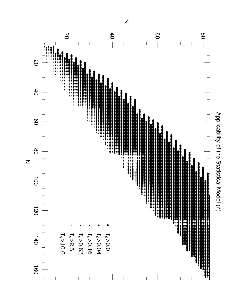
Figure 1: Temperatures (in T₉) for which the statistical model can be used. Plotted is the compound nucleus of the neutron-induced reaction.

The nuclear reaction rate per particle pair at a given stellar temperature $T$ is determined by folding the reaction cross section with the Maxwell-Boltzmann (MB) velocity distribution of the projectiles [10]

$$\left<\sigma v\right>=\left(\frac{8}{\pi\mu}\right)^{1/2}\frac{1}{\left(kT\right)^{3/2}}\int_{0}^{\infty}\sigma(E)E\exp\left(-\frac{E}{kT}\right)dE\quad.$$ (6)

An effective energy window is then found around the peak of the integrand at $E_{0}$. For charged particles this is the so-called Gamow peak at $E_{0}=E_{\mathrm{G}}^{1/3}(kT/2)^{2/3}$ (with the Gamow energy $E_{\mathrm{G}}$). For s-wave neutrons the effective peak coincides with the peak of the MB distribution at $E_{0}=kT$ (close to the neutron separation energy), for higher partial waves the energy window is shifted to slightly higher energies (similarily to the Gamow peak) due to the centrifugal barrier [11]. The effective energy window for a given nucleus and temperature has to contain sufficiently many resonances in order to make it possible to solve the integral with the assumption of an average level density instead of calculating the exact sum over the individual levels. Numerical test calculations [8] have shown that an average number of 5–10 contributing resonances is sufficient. Choosing a lower limit for the number of resonances, determining the width and location of the effective energy window at a given temperature and using the above level density description to calculate the number of resonances in this window, we derive a lower limit for the temperature at which the SM can still be used. Those temperature limits are shown in Fig. 1 for neutron-induced reactions. It should be noted that the derived temperatures will not change considerably even if changing the required level number within a factor of two, because of the exponential dependence of the level density on the excitation energy.

4 SUMMARY

Making use of an improved level density description we presented a method to determine the applicability of the SM, also providing clues on which reactions might be of special interest for experimental investigations. In principle, the method can be used for any projectiles and also with different incident energy distributions (e.g. for experimental beams).

References

- [1] J.J. Cowan, F.-K. Thielemann and J.W. Truran, Phys. Rep. 208 (1991) 267.
- [2] A.H. Bethe, Phys. Rev. 50 (1936) 332.
- [3] A.V. Ignatyuk, G.N. Smirenkin and A.S. Tishin, Yad. Phys. 21 (1975) 485.
- [4] Reisdorf, Z. Phys. A 300 (1981) 227.
- [5] A.S. Iljinov, M.V. Mebel et al., Nucl. Phys. A543 (1992) 517.
- [6] D.J. Dean, S.E. Koonin, K. Langanke et al., Phys. Rev. Lett. 74 (1995) 2909.
- [7] T. Rauscher, F.-K. Thielemann and K.-L. Kratz, Mem. Soc. Astr. Ital., in press.
- [8] T. Rauscher, F.-K. Thielemann and K.-L. Kratz, to be submitted to Phys. Rev. C.
- [9] P. Möller, J.R. Nix et al., At. Data Nucl. Data Tables 59 (1995) 185.
- [10] W.A. Fowler, G.E. Caughlan and B.A. Zimmerman, Ann. Rev. Astron. Astrophys. 5 (1967) 525.
- [11] R.V. Wagoner, Ap. J. Suppl. 18 (1969) 247.