March 4, 1997

IS LENSING OF POINT SOURCES A PROBLEM FOR FUTURE CMB EXPERIMENTS?

Max Tegmark^1,2,3, & Jens V. Villumsen³

¹Institute for Advanced Study, Olden Lane, Princeton, NJ 08540; max@ias.edu
²Max-Planck-Institut für Physik, Föhringer Ring 6, D-80805 München
²Max-Planck-Institut für Astrophysik, Karl-Schwarzschild-Str. 1, D-85740 Garching; jens@mpa-garching.mpg.de

Weak gravitational lensing from large-scale structure enhances and reduces the fluxes from extragalactic point sources with an r.m.s. amplitude of order 15%. In cosmic microwave background (CMB) experiments, sources exceeding some flux threshold ${\phi_{c}}$ are removed, which means that lensing will modulate the brightness map of the remaining unresolved sources. Since this mean brightness is of order $100\mu\hbox{K}$ at 30 GHz for a reasonable flux cut, one might be concerned that this modulation could cause substantial problems for future CMB experiments. We present a detailed calculation of this effect and, fortunately, find that its power spectrum is always smaller than the normal point source power spectrum. Thus although this effect should be taken into account when analysing future high-precision CMB measurements, it will not substantially reduce the accuracy with which cosmological parameters can be measured.

1 INTRODUCTION

Future high-precision measurements of the fluctuations in the cosmic microwave background (CMB) may allow key cosmological parameters (such as $\Omega$, $\Lambda$, $\Omega_{b}$, the Hubble constant, etc.) to be measured with unprecedented accuracy (Jungman et al. 1996; Bond et al. 1997; Zaldarriaga et al. 1997), and a number of ground-, balloon- and space-based missions are currently being planned for this purpose. Both when designing such missions and when analyzing the data sets that they produce, it is important that all relevant sources of foreground contamination are well understood, to minimize the risk that foreground signals are misinterpreted as CMB fluctuations. Since numerous experiments are are currently in the planning and design stages, it is therefore timely to catalog and quantify all possible foreground effects. Figure 1 summarizes recent foreground estimates from Tegmark & Efstathiou (1996), hereafter “TE96”, and Bersanelli et al. (1996). The purpose of this Letter is to investigate yet another foreground effect which has not been previously studied: that of weak gravitational lensing of point sources. In other words, we will discuss the extent to which the point source region (which occupies mainly the lower right corner of Figure 1) is expanded by lensing.

Since it is impossible to remove all point sources (as there are for all practical purposes infinitely many, and not all with the same spectra), the standard procedure in CMB experiments is to remove all point sources below some flux cut ${\phi_{c}}$, either by subtracting their estimated emission or by discarding all contaminated pixels. The total sky brightness from the remaining sources tends to be dominated by faint ones, whereas the brightness fluctuations (which contribute to Figure 1) are dominated by the sources just below the flux cut. For this reason, the average brightness $B$ exceeds the r.m.s. fluctuations by a substantial factor, typically $\sim 10^{3}$, as shown in Figure 2. A process that caused even minor spatial modulations of $B$ could therefore pose a serious problem for CMB experiments.

Weak gravitational lensing by large-scale structure (see Villumsen 1996 for a recent discussion) can affect observed power spectra in more ways than one. If we imagine a pattern painted on the inside of a rubber (celestial) sphere, weak lensing corresponds to stretching and compressing the rubber in a random fashion, much like the way our mirror images get distorted by non-flat mirrors in amusement parks. For weak lensing, this distortion will always constitute a one-to-one mapping of the image, i.e., there will be no caustics where the image “folds over” on itself. There is thus no smearing involved, so the fluctuation power is conserved. Instead, there is a “Robin Hood effect” where power is redistributed between multipoles, from those which have more to those which have less (Seljak 1996). For the CMB power spectrum, this effect is typically a few percent, and may well be detectable in future CMB experiments. For point sources, on the other hand, this effect is completely absent: since they have a Poisson power spectrum with $C_{\l}$ constant, the Robin Hood effect (which effectively simply smoothes the power spectrum), will leave $C_{\l}$ unaffected.

However, the presence of a flux cut for point sources produce a different effect, which is absent for the CMB. In those regions where lensing causes magnification, we will see (and remove) disproportionately many sources above the flux cut (Turner et al. 1984, Broadhurst et al. 1995). Since lensing leaves the average brightness unaffected, the sky brightness from unremoved sources will be lower than average in this region. In other words, weak lensing causes the type of modulation of $B$ that we warned about above. The rest of this Letter is organized as follows. We present a detailed calculation of this effect in Section 2, assess its importance in Section 3 and summarize our findings in Section 4.

2 CALCULATION OF THE EFFECT

2.1 How magnification bias affects the source counts

Let the unlensed source count function ${\bar{n}}(>\phi)$ denote the number of sources per steradian whose flux would exceed $\phi$ in the absence of lensing. When weak gravitational lensing magnifies a patch of sky with a magnification factor $m$, this has two separate effects on ${\bar{n}}(>\phi)$:

• The sources become a factor $m$ brighter.

• The sources are seen further apart, reducing their number density by a factor $m$.

In summary, the lensed source count function, which we denote ${\tilde{n}}(>\phi)$, is given by

$${\tilde{n}}(>\phi)={1\over m}{\bar{n}}\left(>{\phi\over m}\right).$$ (1)

Defining the differential source count as ${\bar{n}}^{\prime}(\phi)\equiv d{\bar{n}}(<\phi)/d\phi=-d{\bar{n}}(>\phi)/d\phi$ (a positive function), we thus have

$${\tilde{n}}^{\prime}(\phi)={1\over m^{2}}{\bar{n}}^{\prime}\left({\phi\over m}\right).$$ (2)

For weak lensing, we can write $m=1+\Delta$, where $|\Delta|\ll 1$ (Broadhurst et al. 1995), and we will make the approximation of dropping all quadratic and higher order terms in $\Delta$. Using ${\bar{n}}^{\prime}(\phi/m)\approx{\bar{n}}^{\prime}(\phi-\phi\Delta)\approx{\bar{n}}^{\prime}(\phi)-{\bar{n}}^{\prime\prime}(\phi)\phi\Delta$, we can rewrite equation (2) as

$${\tilde{n}}^{\prime}(\phi,\widehat{{\bf r}})={\bar{n}}^{\prime}(\phi)-{1\over\phi}\left[{\bar{n}}^{\prime}(\phi)\phi^{2}\right]^{\prime}\Delta(\widehat{{\bf r}}),$$ (3)

where we have explicitly indicated the fact that the magnification field depends on $\widehat{{\bf r}}$, the unit vector pointing in our direction of observation.

Since the total sky brightness $\int_{0}^{\infty}{\bar{n}}^{\prime}\phi d\phi$ is finite, the quantity ${\bar{n}}^{\prime}\phi^{2}$ must clearly approach zero both as $\phi\to 0$ and as $\phi\to\infty$, otherwise the integral would diverge at the faint or bright end. Since the second term in equation (3) becomes a total differential when multiplied by $\phi$, this means that the total brightness is not affected by lensing. This well-known fact is also verified by integrating $\phi$ times equation (2) and changing variables. However, when the upper integration limit is not $\infty$, the same procedure shows that the brightness contribution from all sources below some fixed flux cut is affected by lensing, and we will now evaluate this effect.

2.2 The effect on the point source correlation function

For CMB purposes, we can to a good approximation (TE96) model the locations of extragalactic point sources as completely uncorrelated. In the absence of lensing, we can therefore write the observed density of point sources above some flux cut ${\phi_{c}}$ as a sum of angular delta functions, $n(\widehat{{\bf r}})=\sum\delta(\widehat{{\bf r}},\widehat{{\bf r}}_{i})$, and model $n(\widehat{{\bf r}})$ as a Poisson process. A Poisson process satisfies (see e.g. Appendix A of Feldman, Kaiser & Peacock 1994)

$$\langle n(\widehat{{\bf r}})\rangle_{p} = {\bar{n}}(\widehat{{\bf r}}),$$ (4)

$$\langle n(\widehat{{\bf r}})n(\widehat{{\bf r}}^{\prime})\rangle_{p} = {\bar{n}}(\widehat{{\bf r}}){\bar{n}}(\widehat{{\bf r}}^{\prime})+\delta(\widehat{{\bf r}},\widehat{{\bf r}}^{\prime}){\bar{n}}(\widehat{{\bf r}}).$$ (5)

We use $\langle\>\rangle_{p}$ to denote ensemble averages with respect to the Poisson process, to distinguish these from ensemble averages with respect to the random field $\Delta$, which we will denote by $\langle\>\rangle_{f}$. When performing both averages below, we will omit subscripts and write $\langle\>\rangle=\langle\langle\>\rangle_{p}\rangle_{f}$.

Magnification bias forces us to take into account that the total source population is the union of a number of independent subpopulations, corresponding to different flux classes. We therefore write

$$n(\widehat{{\bf r}})=\int_{0}^{\phi_{c}}n^{\prime}(\phi,\widehat{{\bf r}})d\phi,$$ (6)

where $n^{\prime}(\phi,\widehat{{\bf r}})d\phi$ is a sum of delta functions corresponding to the sources whose fluxes fall between $\phi$ and $\phi+d\phi$. With this notation, equations (4) and (5) become generalized to

$$\langle n^{\prime}(\phi,\widehat{{\bf r}})\rangle_{p} = {\tilde{n}}^{\prime}(\phi,\widehat{{\bf r}}),$$ (7)

$$\langle n^{\prime}(\phi,\widehat{{\bf r}})n^{\prime}(\phi^{\prime},\widehat{{\bf r}}^{\prime})\rangle_{p} = {\tilde{n}}^{\prime}(\phi,\widehat{{\bf r}}){\tilde{n}}^{\prime}(\phi^{\prime},\widehat{{\bf r}}^{\prime})+\delta(\phi-\phi^{\prime})\delta(\widehat{{\bf r}},\widehat{{\bf r}}^{\prime}){\tilde{n}}^{\prime}(\phi,\widehat{{\bf r}}).$$ (8)

The observed sky brightness $x$ in a direction $\widehat{{\bf r}}$ is clearly given by

$$x(\widehat{{\bf r}})\equiv\int_{0}^{\phi_{c}}n^{\prime}(\phi,\widehat{{\bf r}})\phi d\phi,$$ (9)

and we will now calculate its statistical properties.

Using equations (3), (7) and (9), we see that the mean is given by

$$\langle x(\widehat{{\bf r}})\rangle=\int_{0}^{\phi_{c}}\langle\langle n^{\prime}(\phi,\widehat{{\bf r}})\rangle_{p}\rangle_{f}\phi d\phi=B-\langle f(\widehat{{\bf r}})\rangle_{f},$$ (10)

where we have defined

$$f(\widehat{{\bf r}})\equiv{\bar{n}}^{\prime}({\phi_{c}}){\phi_{c}}^{2}\Delta(\widehat{{\bf r}})$$ (11)

and where $B$ denotes the average total brightness due to sources below our flux cut, i.e.,

$$B\equiv\int_{0}^{\phi_{c}}{\bar{n}}^{\prime}(\phi)\phi d\phi.$$ (12)

Since $\langle\Delta(\widehat{{\bf r}})\rangle_{f}=0$ (there is just as much positive as negative weak lensing from large-scale structure), the second term in equation (10) vanishes, and we see that regardless of the flux cut, lensing has no impact on the average brightness of unremoved point sources.

We now turn to the correlation function. Using $\langle\Delta(\widehat{{\bf r}})\rangle_{f}=0$ and equations (3), (7), (8) and (9), we obtain

$$\langle x(\widehat{{\bf r}})x(\widehat{{\bf r}}^{\prime})\rangle = \int_{0}^{\phi_{c}}\int_{0}^{\phi_{c}}\langle\langle n^{\prime}(\phi,\widehat{{\bf r}})n^{\prime}(\phi^{\prime},\widehat{{\bf r}}^{\prime})\rangle_{p}\rangle_{f}\phi\phi^{\prime}d\phi d\phi^{\prime}$$ (13)

$$= \langle[B-f(\widehat{{\bf r}})][B-f(\widehat{{\bf r}}^{\prime})]\rangle_{f}+\delta(\widehat{{\bf r}},\widehat{{\bf r}}^{\prime})C^{ps},$$

where

$$C^{ps}\equiv\int_{0}^{\phi_{c}}{\bar{n}}^{\prime}(\phi)\phi^{2}d\phi$$ (14)

is the familiar power spectrum of unresolved point sources in the absence of lensing that was derived in TE96. Using $\langle f(\widehat{{\bf r}})\rangle_{f}=0$ again, this reduces to

$$\langle x(\widehat{{\bf r}})x(\widehat{{\bf r}}^{\prime})\rangle=B^{2}+C^{ps}+{\bar{n}}^{\prime}({\phi_{c}})^{2}{\phi_{c}}^{4}\langle\Delta(\widehat{{\bf r}})\Delta(\widehat{{\bf r}}^{\prime})\rangle_{f}.$$ (15)

Since the first term is merely the familiar and uninteresting monopole, the new effect that we have computed corresponds to the third term. Thus the effect of lensing is to add to the original point source correlation function a new term which is the magnification correlation times ${\bar{n}}^{\prime}({\phi_{c}})^{2}{\phi_{c}}^{4}$.

2.3 The effect on the point source power spectrum

Let us expand the sky brightness $x$ in spherical harmonics and investigate the statistical properties of the expansion coefficients

$$a_{\l m}\equiv\int Y_{\l m}^{*}(\widehat{{\bf r}})x(\widehat{{\bf r}})d\Omega.$$ (16)

Assuming that the statistical properties of the magnification field $\Delta$ are isotropic (there is no need to assume that $\Delta$ is Gaussian), its corresponding expansion coefficients $\Delta_{\l m}$ must satisfy

$$\langle\Delta_{\l m}^{*}\Delta_{\l^{\prime}m^{\prime}}\rangle_{f}=\delta_{\l\l^{\prime}}\delta_{mm^{\prime}}C_{\l}^{mag}$$ (17)

for some $C_{\l}^{mag}$ which we will refer to as the magnification power spectrum. Substituting equation (15) into

$$\langle a_{\l m}^{*}a_{\l^{\prime}m^{\prime}}\rangle=\int\int Y_{\l m}^{*}(\widehat{{\bf r}})Y_{\l^{\prime}m^{\prime}}(\widehat{{\bf r}}^{\prime})\langle x(\widehat{{\bf r}})x(\widehat{{\bf r}}^{\prime})\rangle d\Omega d\Omega^{\prime},$$ (18)

we obtain

$$\langle a_{\l m}^{*}a_{\l^{\prime}m^{\prime}}\rangle=\delta_{\l\l^{\prime}}\delta_{mm^{\prime}}C_{\l},$$ (19)

where the point source power spectrum is

$$C_{\l}=4\pi\delta_{0\l}\delta_{0m}B^{2}+C^{ps}+{\bar{n}}^{\prime}({\phi_{c}})^{2}{\phi_{c}}^{4}C_{\l}^{mag}.$$ (20)

The first two terms are merely the monopole and the shot noise power (which is independent of $\l$), derived in TE96, so the new effect due to lensing is given by the third term.

3 HOW IMPORTANT IS THE NEW EFFECT?

3.1 Some useful approximations

To clarify the relative importance of the last two terms in equation (20), it is convenient to express them in terms of quantities that are more directly linked to observations. For typical scenarios, the differential source count ${\bar{n}}^{\prime}(\phi)$ is a smooth function on a log-log-plot, which means that near the flux cut ${\phi_{c}}$, we can approximate it with a power law

$${\bar{n}}^{\prime}(\phi)\approx{\bar{n}}^{\prime}({\phi_{c}})\left({\phi\over{\phi_{c}}}\right)^{-\beta}$$ (21)

for some constant $\beta$. To avoid the above-mentioned divergence of the total brightness, we must have a logarithmic slope $\beta<2$ at the faint end and $\beta>2$ at the bright end. For instance, for radio sources at 1.5 GHz, the VLA FIRST survey gives the logarithmic slope $\beta\sim 1.6$ at ${\phi_{c}}\sim$ 1 mJy, steepening to $\beta\sim 2.5$ at the bright end (White et al. 1996, TE96) just as one would expect if the brightest sources are at low redshifts $z\ll 1$ where evolutionary and cosmological effects are negligible, and the same qualitative behavior is found at higher frequencies (Windhorst et al. 1985, 1993). Using equation (21), we thus find that the expected number $N$ of sources above the flux cut is

$$N\equiv 4\pi\int_{\phi_{c}}^{\infty}{\bar{n}}^{\prime}(\phi)d\phi\approx{4\pi\over\beta-1}{\phi_{c}}{\bar{n}}^{\prime}({\phi_{c}})\propto{\phi_{c}}^{-(\beta-1)},$$ (22)

since the integral is dominated by sources just above the flux cut for which the power law fit is very accurate. Similarly, the integral in equation (14) is dominated by sources just below the cut, so using equations (21) and (22) gives

$$C^{ps}\approx\left({\beta-1\over 3-\beta}\right)\left({N\over 4\pi}\right){\phi_{c}}^{2}\propto{\phi_{c}}^{3-\beta}.$$ (23)

Finally, we can rewrite the lensing term in equation (20) as

$${\bar{n}}^{\prime}({\phi_{c}})^{2}{\phi_{c}}^{4}C_{\l}^{mag} \approx (\beta-1)^{2}\left({N\over 4\pi}\right)^{2}{\phi_{c}}^{2}C_{\l}^{mag}$$ (24)

$$\approx (\beta-1)(3-\beta)\left({N\over 4\pi}\right)C_{\l}^{mag}C^{ps}$$

$$\propto {\phi_{c}}^{-2(\beta-2)}.$$

Equation (20) showed that that power spectrum was a sum of three different terms. These are all plotted in Figure 2 as a function of the flux cut, using the source counts ${\bar{n}}^{\prime}(\phi)$ from the VLA FIRST survey (White et al. 1996). The approximations above allow us to understand all qualitative features of this figure. Comparing equations (23) and (24), we notice that although the Poisson term $C^{ps}$ decreases if we remove more sources, the lensing term increases as long as $\beta>2$, i.e., as long as we remove less than $\sim 10^{5}$ sources from an all-sky survey, or $\sim 4$ sources per square degree. This corresponds to $\sim 60$ sources in a $4^{\circ}\times 4^{\circ}$ field of the upcoming Very Small Array (VSA) experiment, and to a 50 mJy flux cut at 1.5 GHz.

3.2 The magnification power spectrum

Equation (24) shows that when $\beta\approx 2$, the ratio between the lensing term and the conventional shot noise term $C^{ps}$ is simply $C_{\l}^{mag}$ times $N/4\pi$, the number of removed sources per steradian. $N/4\pi$ is typically $\gg 1$, and we will now evaluate $C_{\l}^{mag}$. For any flat Friedman-Robertson-Walker cosmology, including non-linear clustering and an arbitrary source distribution $n(x_{s})$, the magnification power spectrum is given by (Villumsen 1996)

$$C_{\l}^{mag}=72\pi^{3}\Omega_{0}^{2}d^{-3}\int_{0}^{x_{h}}w^{2}(x_{l})(1+z)^{2}P(\l/yd,z)\ dx_{l},$$ (25)

where the function $w$ is defined as

$$w(x_{l})\equiv\int_{x_{l}}^{x_{h}}{y_{ls}\over y_{s}}n(x_{s})\ dx_{s}.$$ (26)

Here $d\equiv H_{0}^{-1}c\approx 3000h^{-1}{\rm Mpc}$, $P(k,z)$ is the conventional three-dimensional matter power spectrum at redshift $z$, and $xd$ and $yd$ are the comoving radial and angular distances to the epoch $z$, respectively. Subscripts $h$, $l$ and $s$ refer to horizon, lens and source positions, respectively, and $y_{ls}$ is the comoving angular lens-source distance. These equations are valid on angular scales where the sky is approximately flat, i.e., $\l\gg 60$, which is of course the case in our regime of interest. For the simple case where $\Omega=1$, $\Lambda=0$, the density fluctuations grow according to linear theory and all sources are located at some characteristic redshift $z_{s}$, this reduces to

$$C_{\l}^{mag}=72\pi^{3}d^{-3}\int_{0}^{x_{s}}\left(1-{x\over x_{s}}\right)^{2}P\left({\l\over xd}\right)\,dx,$$ (27)

where $P$ is the current power spectrum and $x_{s}=2-2/\sqrt{1+z_{s}}$.

Parameter	Opt.	Mid.	Pess.
Source redshift	0.4	1	$\gg$1
$\alpha$	0.2	0	$-$0.3
$\Omega_{0}\sigma_{8}$	0.2	0.7	1
Removed/sq deg	0.5	2	4
$\beta({\phi_{c}})$	2.5	2.2	2

Table 1: Parameters used in optimistic, middle-of-the-road and pessimistic scenarios.

This is plotted in Figure 3 (dashed curves) for a standard CDM power spectrum (Bond & Efstathiou 1984) with $h=0.5$, for the three cases described in Table 1. We label these scenarios “pessimistic”, “middle-of-the-road” and “optimistic”, since they are intended to give an upper limit, realistic estimate and lower limit, respectively, as to how much of a problem the lensing effect will turn out to be for future CMB experiments. Apart from a factor of $\ln 10$, the magnification fluctuation on a given scale is essentially the area under a plotted curve out to that scale. For instance, the r.m.s. magnification fluctuations after smoothing on a scale of 5 arcminutes is about $15\%$ for the pessimistic model, where the sources that have the dominant effect on the CMB are assumed to be at redshifts $\gg 1$. However, what matters for our purposes is of course not this r.m.s. magnification fluctuation, but $C_{\l}^{mag}$ itself. In the pessimistic scenario, the maximum power is $C_{\l}^{mag}\sim\times 10^{-6}$, attained for $\l\sim 10^{2}$, which ensures that the r.m.s. lensing fluctuations are below the standard Poisson fluctuations for any reasonable flux cut.

3.3 The uncertain point source normalization

This conclusion in independent of the overall normalization of the point source counts ${\bar{n}}^{\prime}(\phi)$, since Equation (24) shows that the ratio of our lensing effect to the shot noise power $C^{ps}$ is independent of this normalization. However, to assess the overall importance of both effects to future CMB experiments, accurate knowledge of the radio source counts at the frequencies where the observations are made is crucial. Unfortunately, the point source population between 20 and a few hundred GHz is still very poorly determined (see e.g. Gundersen et al. 1997), leaving open only the unattractive option of extrapolating from lower frequencies. In Figure 3 we have extrapolated the 1.5 GHz VLA FIRST data to 30 GHz by assuming that the temperature fluctuations $(C^{ps})^{1/2}(\nu)\propto\nu^{-(2+\alpha)}$. To reflect the observational uncertainty, we have allowed $\alpha$ to vary as shown in Table 1, with the middle-of-the-road estimate being that of TE96.

4 CONCLUSIONS

We have calculated the effect of weak gravitational lensing on the power spectrum of unresolved point sources. We found that this adds a new term, which is the magnification power spectrum times ${\bar{n}}^{\prime}({\phi_{c}})^{2}{\phi_{c}}^{4}$. The ratio between this term and the standard Poisson term is roughly $(N/4\pi)C_{\l}^{mag}$, independent of the (poorly known) point source normalization, so if we keep shrinking the point source region in Figure 1 by lowering the flux cut ad infinitum, the lensing term will eventually become the dominant problem. The lensing term initially increases as we remove more sources, reaching a maximum when $\sim 4$ sources per square degree are removed.

Figure 1 shows that for high-resolution interferometric experiments operating at low frequencies, a fairly aggressive source removal scheme will be necessary, bringing the lensing effect close to this maximum strength. Effective point source removal will be important for the future Satellite missions MAP and Planck as well. Fortunately, this strength does not exceed 12% of the standard Poisson fluctuations even in the worst-case scenario.

In summary, although this effect should be taken into account in the detailed analysis of some future CMB experiments, it is likely to be a relatively small correction (like, e.g., the Rees-Sciama effect) and should not substantially reduce the accuracy with which cosmological parameters can be measured.

The authors wish to thank Avi Loeb for suggesting this project and for helpful comments on the manuscript. This work was partially supported by European Union contract CHRX-CT93-0120, by Deutsche Forschungsgemeinschaft grant SFB-375 and by NASA through a Hubble Fellowship, #HF-01084.01-96A, awarded by the Space Telescope Science Institute, which is operated by AURA, Inc. under NASA contract NAS5-26555.

5 REFERENCES

Bersanelli, M. et al. 1996, COBRAS/SAMBA report on the phase A study, ESA report D/SCI(96)3.

Bond, J. R. & Efstathiou, G. 1984, ApJ, 285, L45.

Bond, J. R., Efstathiou, G. & Tegmark, M. 1997, preprint astro-ph/9702100

Broadhurst, T. J., Taylor, A. N. & Peacock, J. A. 1995, ApJ, 438, 49.

Feldman, H. A., Kaiser, N. & Peacock, J. A. 1994, ApJ, 426, 23.

Gundersen, J. O., Staveley-Smith, P., Payne, P. & Lubin, P. M. 1997, submitted to ApJL.

Jungman, G.. Kamionkowski, M., Kosowsky, A & Spergel, D. N. 1996, Phys. Rev. D, 54, 1332.

Seljak, U. 1996, ApJ, 463, 1.

Tegmark, M. & Efstathiou, G. 1996, MNRAS, 281, 1297 (“TE96”).

Turner, E., Ostriker, J. P. & Gott, J. R. III 1984, ApJ, 284, 1.

Villumsen, J. V. 1996, MNRAS, 281, 369.

Windhorst, R. A., Miley, G. K., Owen, F. N., Kron, R. G. & Koo, D. C. 1985, ApJ, 289, 494.

Windhorst, R.A., Fomalont, E.B., Partridge, R.B., & Lowenthal 1993, ApJ, 405, 498.

White, R. L., Becker, R. H., Helfand, D. J. & Gregg, M. D. 1996, submitted to ApJ.

Zaldarriaga, M., Spergel, D. & Seljak, U. 1997, preprint astro-ph/9702157

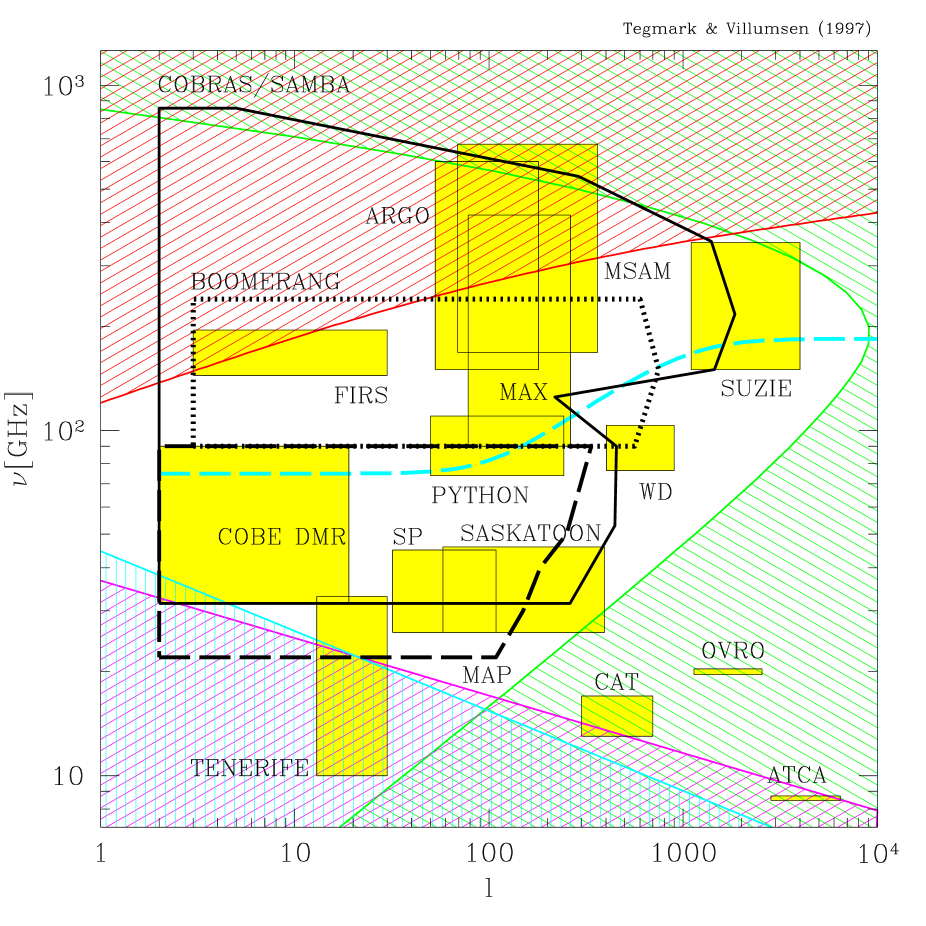
Figure 1: Where various foregrounds dominate.

The shaded regions indicate where the various foregrounds cause fluctuations exceeding those of COBE-normalized scale-invariant fluctuations, thus posing a substantial challenge to estimation of genuine CMB fluctuations. They correspond to dust (top), free-free emission (lower left), synchrotron radiation (lower left, vertically shaded) and point sources (lower and upper right). The heavy dashed line shows the frequency where the total foreground contribution to each multipole is minimal. The boxes roughly indicate the range of multipoles $\l$ and frequencies $\nu$ probed by various CMB experiments, as in TE96.

Figure 2: Dependence of radio source fluctuations on flux cut.

The three terms that contribute to the point source power spectrum in equation (20) are plotted as a function of the number of sources removed in an all-sky survey (only the number per steradian matters), based on the VLA FIRST source counts. These terms (solid curves) are the integrated brightness of the population, the edge effect at the flux cut and the shot noise fluctuations, respectively. The dashed curves show the lensing contribution to $C_{\l}^{1/2}$ for the pessimistic and middle-of-the-road scenarios, at the worst-case $\l$-values.

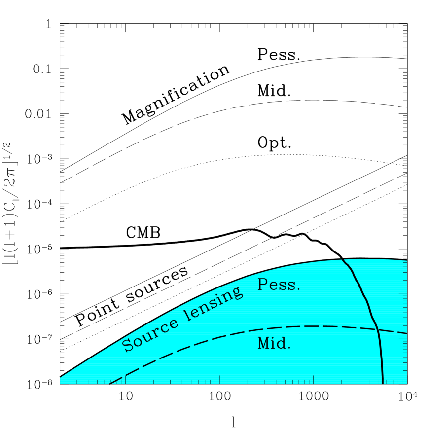
Figure 3: The power spectra are plotted for the CMB (heavy line), the lensing magnification field (the three top lines), discrete point sources at 30 GHz (the three straight lines) and the lensing effect on them (the two bottom lines), all for a standard CDM model. The solid, dashed and dotted lines correspond to the pessimistic, middle-of-the-road and optimistic scenarios, respectively.