A New Statistic for Redshift Surveys:
the Redshift Dispersion of Galaxies

Abstract

We present a new statistic—the redshift dispersion— which may prove useful for comparing next generation redshift surveys (e.g., the Sloan Digital Sky Survey) and cosmological simulations. Our statistic is specifically designed for the projection of phase space which is directly measured by redshift surveys. We find that the redshift dispersion of galaxies as a function of the projected overdensity has a strong dependence on the cosmological density parameter $\Omega$. The redshift dispersion statistic is easy to compute and can be motivated by applying the Cosmic Virial Theorem to subsets of galaxies with the same local density. We show that the velocity dispersion of particles in these subsets is proportional to the product of $\Omega$ and the local density. Low resolution N-body simulations of several cosmological models (open/closed CDM, CDM+$\Lambda$, HDM) indicate that the proportionality between velocity dispersion, local density and $\Omega$ holds over redshift scales in the range 50 ${\rm km~{}s^{-1}}$ to 500 ${\rm km~{}s^{-1}}$. The redshift dispersion may provide an interesting means for comparing volume-limited subsamples of the Sloan Digital Sky Survey to equivalent N-body/hydrodynamics simulations.

1 Introduction

Many statistical measures have been developed to distinguish between the various cosmological models, ranging from direct measures of the power spectrum and correlation function from redshift surveys, to measures of velocity dispersion, bulk flows, and Mach number from peculiar velocity surveys (cf., Strauss & Willick (1995) for a review). Each of these measures is designed to be sensitive to different aspects of various models, such as $\Omega$, the initial power spectrum, or the Gaussian character of the initial phase distribution.

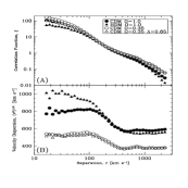
Figure 1: Two-point correlation function (a) and pairwise velocity dispersion (b) measured in N-body simulations of four cosmological models. Each model was normalized to have similar power on small scales (i.e., $\sigma_{8}=0.67$).

One can get an intuitive understanding of the dependencies of different statistics by considering the following example. Compare N-body simulations of four different cosmological models: standard CDM, open CDM, CDM + $\Lambda$, and a pure HDM model, the details of which are given in §3. Each simulation is normalized to have the same value of $\sigma_{8}$, the standard deviation of the mass fluctuations within an 8 ${h^{-1}{\rm Mpc}}$ sphere, where $h$ is the Hubble parameter in units of 100 ${\rm km~{}s^{-1}}~{}{\rm Mpc}^{-1}$. The two point correlation function, $\xi(r)$, for each model is presented in Figure 1a. Despite their differences in initial power spectra, the final correlation functions are similar in all models. In general, the correlation function does not depend strongly on $\Omega$ if one retains the freedom to set the $\sigma_{8}$ normalization. In contrast, Figure 1b shows the pairwise velocity dispersion, $\langle v^{2}\rangle(r)$, as a function of separation for the same set of models. A strong differentiation between the low and high $\Omega$ models is apparent.

The velocity dispersion is easy to compute in simulations, but is difficult to measure in the geometric projection of phase space that is measured by redshift surveys. The traditional way to measure the small-scale velocity dispersion of galaxies is via the anisotropy it introduces in the redshift-space two-point correlation function (Davis & Peebles (1983); Fisher et al. (1994); Marzke et al. (1995); Loveday et al. (1996)). However, as it is a pair-weighted statistic, it is dominated by the densest regions, which are necessarily rare. Thus one finds large variance between estimates of the small-scale velocity dispersion between different samples (Mo, Jing, & Börner (1993); Zurek et al. (1994); Guzzo et al. (1996); Somerville, Davis, & Primack (1997)), indicating that the small-scale velocity dispersion measured in this way is not very robust. Attempts have been made to use direct measures of peculiar velocities of galaxies as a constraint on $\langle v^{2}\rangle$ (e.g., Strauss, Cen, & Ostriker (1993), Willick et al. (1997)), but other than the nearby universe, where the velocity field is observed to be very quiet (Sandage (1986); Brown & Peebles (1987); Burstein (1990)), the errors on the individual peculiar velocity measurements swamp the signal from $\langle v^{2}\rangle$.

The primary goal of this paper is to present a statistic—the redshift dispersion (${\sigma_{z}}$)—that captures ${\langle v^{2}\rangle}$ in a way which is naturally applied to volume limited samples drawn from redshift surveys. In the subsequent sections we motivate and present our redshift dispersion statistic. Again, because it is a pair-weighted statistic, computing ${\langle v^{2}\rangle}$ by averaging over all densities results in a value heavily weighted by the densest regions. However, this problem can be alleviated if the dispersion can be calculated as a function of density. The theoretical motivation for our statistic stems from the Cosmic Virial Theorem (CVT), derived in Peebles (1976a, hereafter P76), which relates ${\langle v^{2}\rangle}$ to ${\Omega}$ and $\xi$. In §2 we show that the CVT can be applied to subsets of particles in a system which correspond to surfaces of constant density. Many assumptions are necessary to obtain the results shown in §2, not all of which are obvious. In §3 we explore the relationships derived in §2 with simple N-body simulations, suggesting that the results of §2 hold over a wide range of scales. The redshift dispersion is entirely independent of the results of §2 and §3, which provide a context for the redshift dispersion that would otherwise be an unmotivated simulation based statistic. §4 describes how to compute the redshift dispersion from a redshift survey. §5 contains our conclusions and remarks on future work.

2 Velocity Dispersion on Surfaces of Constant Density

As will be shown in §4, the redshift dispersion probes the pairwise peculiar velocity dispersion in regions of different density and is designed for comparing simulated and observed redshift surveys. In this section we attempt to provide a theoretical context and some motivation.

One of the main challenges of working with the pairwise velocity dispersion arises from its strong density dependence. Intuitively, both the number of galaxies and the velocity dispersion should be highest in the densest regions. Thus, averaging over all densities will give results dominated by rare, high density peaks. This problem can be eliminated if the dispersion is calculated as a function of density.

In the case of clustered, gravitationally interacting particles there exists a scaling relation between the velocity dispersion on small scales ${\langle v^{2}\rangle}(r)$ averaged over pairs separated by a distance $r$, and the two point correlation function $\xi(r)$, the excess fractional probability of finding two particles with separation $r$. This result is contained in the CVT derived in P76 (see also Peebles 1976b ; Davis & Peebles (1977); Peebles (1980)), which can be written

$${\langle v^{2}\rangle}(r)\propto{\Omega}\xi(r)r^{2}.$$ (1)

Several assumptions are used to obtain Eq. (1) (see P76), including that $\xi$ is given by a power law $\xi(r)=(r_{0}/r)^{\gamma}$; $r\ll r_{0}$, implying $\xi(r)\gg 1$; the three-point correlation function $\zeta$ is given by a symmetrized product of the two-point correlation function (see Eq. [A23]); and the mass of each galaxy is concentrated on scales smaller than their separation. The validity of these assumptions is not obvious (Fisher et al. (1994)). For an excellent discussion of the implications of extended dark matter halos on the CVT, see Bartlett & Blanchard (1996). In addition, we are assuming that the galaxy velocity field is unbiased with respect to that of the dark matter. While theoretical investigations have given strong suggestions that a velocity bias of order 20–30% may exist (Couchman & Carlberg (1992), Evrard, Summers, & Davis (1994), Gelb & Bertschinger (1994)), the difficulty in reliably tracing galaxies in simulations has prevented a good estimate of its magnitude (Summers, Davis, & Evrard (1995)). For the motivational purposes of this paper, let us keep these assumptions as we work to derive the density dependence of the CVT.

To rewrite Eq. (1) in terms of the density requires some new notation. Let $\xi_{a\times b}(r)$ denote the cross-correlation of particle sets $a$ and $b$. The two-point (auto) correlation function of all particles in a system ${\cal P}$ can be written $\xi_{{{\cal P}\!\times\!{\cal P}}}(r)$. The correlation function can also be written as the average of the individual cross correlations

$$\xi(r)={1\over N_{{\cal P}}}\sum_{i\in{\cal P}}\xi_{{i\!\times\!{\cal P}}}(r),$$ (2)

where $N_{{\cal P}}$ is the total number of particles. We can write down a similar expression for the velocity dispersion

$${\langle v^{2}\rangle}(r)={1\over N_{{\cal P}}}\sum_{i\in{\cal P}}{\langle v_{{i\!\times\!{\cal P}}}^{2}\rangle}(r),$$ (3)

where ${\langle v_{{i\!\times\!{\cal P}}}^{2}\rangle}(r)$ is the variance of the pairwise velocity between particle $i$ and all particles in ${\cal P}$ which lie a distance $r$ from $i$. We show in Appendix A that these expressions lead to a generalization of the CVT that holds for each particle:

$${\langle v_{{i\!\times\!{\cal P}}}^{2}\rangle}(r)\propto{\Omega}\xi_{{i\!\times\!{\cal P}}}(r)r^{2}.$$ (4)

If the CVT holds for each particle, then it holds for any subset, ${\cal S}\subset{\cal P}$:

$${\langle v_{{{\cal S}\!\times\!{\cal P}}}^{2}\rangle}(r)\propto{\Omega}\xi_{{{\cal S}\!\times\!{\cal P}}}(r)r^{2},$$ (5)

where

$${\langle v_{{{\cal S}\!\times\!{\cal P}}}^{2}\rangle}(r)\equiv{1\over N_{\cal S}}\sum_{i\in{\cal S}\subset{\cal P}}{\langle v_{{i\!\times\!{\cal P}}}^{2}\rangle}(r),$$ (6)

and

$$\xi_{{{\cal S}\!\times\!{\cal P}}}(r)\equiv{1\over N_{\cal S}}\sum_{i\in{\cal S}\subset{\cal P}}\xi_{{i\!\times\!{\cal P}}}(r).$$ (7)

Let $N_{i}(r)$ be the number of particles within a radius $r$ of the $i$th particle, and ${\cal S}_{n}$ the set of all particles for which $N_{i}=n$. For this subset, the CVT is

$${\langle v^{2}\rangle}(n,r)=C_{1}{\Omega}\xi(n,r)r^{2},$$ (8)

where ${\langle v^{2}\rangle}(n,r)\equiv{\langle v_{{{\cal S}_{n}\!\times\!{\cal P}}}^{2}\rangle}(r)$, $\xi(n,r)\equiv\xi_{{{\cal S}_{n}\!\times\!{\cal P}}}(r)$ and $C_{1}$ is given by Eq. (A32). The quantity $\xi(n,r)$ is related to the expected number of particles within a radius $r$ around any particle by

$${\bar{\nu}}\int_{0}^{r}[1+\xi(n,r^{\prime})]4\pi r^{\prime 2}dr^{\prime}=n,$$ (9)

where ${\bar{\nu}}$ is the mean number of particles per unit volume. If $\xi(n,r)\propto r^{-\gamma}$ and $\xi(n,r)\gg 1$ (as assumed in the original P76 derivation), the above expression yields

$${3\over{3-\gamma}}\xi(n,r){\bar{n}}(r)=n,$$ (10)

where ${\bar{n}}(r)\equiv{\bar{\nu}}\frac{4}{3}\pi r^{3}$.

Inserting the above expression into Eq. (8) yields

$${\langle v^{2}\rangle}(n,r)=C_{1}C_{2}{\Omega}n/{\bar{n}}(r)^{1/3},$$ (11)

where $C_{2}=(3-\gamma)/3(4\pi{\bar{\nu}}/3)^{2/3}$. The above expression shows that the pairwise velocity dispersion is proportional to ${\Omega}$ and the local density (through $n$) smoothed on a scale $r$. Finally, since we are working with $N_{i}(r)$, which is the number of particles within a volume of radius $r$ centered on a particle, it is convenient to work with a similar velocity dispersion. Let ${\sigma_{v}^{2}}(r)$ be the average pairwise velocity dispersion of all the particles within a volume of radius $r$. ${\sigma_{v}^{2}}(r)$ can be obtained by integrating ${\langle v^{2}\rangle}(r)$ under the same assumptions used to derive Eq. (1)

$${\sigma_{v}^{2}}(r)\equiv\frac{\int_{0}^{r}{\langle v^{2}\rangle}(r^{\prime})[1+\xi(r^{\prime})]4\pi r^{\prime 2}dr^{\prime}}{\int_{0}^{r}[1+\xi(r^{\prime})]4\pi r^{\prime 2}dr^{\prime}}=C_{1}C_{3}\frac{{\Omega}\xi(r)^{2}r^{5}}{r^{3}\xi(r)}=C_{3}{\langle v^{2}\rangle}(r),$$ (12)

where $C_{3}=(3-\gamma)/(5-2\gamma)$. Substituting Eq. (12) into (11) results in

$${\sigma_{v}^{2}}(n,r)\propto{\Omega}n/{\bar{n}}(r)^{1/3}$$ (13)

where the constant of proportionality is equal to

$$C_{1}C_{2}C_{3}=\frac{3{\Omega}QM_{\gamma}(3-\gamma)^{2}}{4(\gamma-1)(2-\gamma)(4-\gamma)(5-2\gamma)(4\pi{\bar{\nu}}/3)^{2/3}},$$ (14)

and $Q$ and $M_{\gamma}$ are defined in Appendix A.

The above derivation of Eq. (13) holds whether or not the quantities are averaged over one or many particles with the same density. The above velocity dispersion is computed with respect to the velocity of the central particle, ${\bf{v}}$. The velocity dispersion can also be computed with respect to the mean velocity of the particles in a cell, ${\bf{u}}$. In a given cell, these two values of the velocity dispersion will differ by $|{\bf{u}}|^{2}-|{\bf{v}}|^{2}$. The distribution of these differences for all cells in ${\cal S}_{n}$ will peak at zero and have a width on the order of ${\sigma_{v}^{2}}$. Subsequent averaging over many cells with the same density will result in zero net difference. Thus, Eq. (13) also applies for velocity dispersions computed with respect to the mean velocity in the cell if the results are averaged over many cells in ${\cal S}_{n}$.

Eq. (13) conveniently relates two readily computable quantities: the velocity dispersion with respect to the mean velocity in a cell of radius $r$ to the number of particles in the cell, which is proportional to the density. In the next section, we explore the above form of the CVT with N-body simulations.

3 N-Body Results

The previous section presented a derivation for a relationship linking the velocity dispersion to the local density. In this section we explore the range over which Eq. (13) holds using N-body simulations of specific cosmological models with different initial power spectra. We are particularly interested in the dependence on ${\Omega}$ when the number of objects is of the same order as expected from volume limited redshift surveys.

The simulations we consider are designed to probe a variety of popular cosmological models. The four models are: standard CDM with $\Omega=1$, $h=0.5$; HDM with $\Omega=1$, $h=1.0$; open CDM with $\Omega=0.35$, $h=0.7$; and CDM + $\Lambda$ with $\Omega_{CDM}=0.35$, $\Omega_{\Lambda}=0.65$, $h=0.7$. The open CDM and CDM + $\Lambda$ models provide two alternatives to standard CDM that increase the ratio of large scale to small scale power. They differ in evolution in that structure formation “freezes out” at an earlier epoch in the open model as the expansion rate exceeds the rate of gravitational collapse. Thus, to achieve the same level of structure today, collapse must begin earliest in the open CDM model, later in the CDM + $\Lambda$ model, and latest in standard CDM model. While HDM is not generally considered a viable theory, it provides a significantly different power spectrum shape with which to explore our ideas.

The initial conditions are designed to treat the models, as much as possible, on an even footing. All models assume a Harrison-Zel’dovich primordial power spectrum, and use the same random phases for the Fourier modes to generate the initial density field from their respective power spectra. The CDM transfer functions are taken from Efstathiou, Bond, & White (1992, Eq. [7]) with the parameter $\Gamma\equiv\Omega_{CDM}\,h$. Although this function was not intended for use in open models, it fits more detailed calculations to within 5% (D. N. Spergel 1995, private communication). The HDM transfer function is taken from Holtzman (1989, Table 2A, line 52). As stated in §1, each model is normalized to have the same linear value of $\sigma_{8}=0.67$, so as to provide similar correlation strengths and to isolate out the velocity dependencies. Although this normalization does not match that predicted from the observed fluctuations in the Cosmic Microwave Background for some or all of the models (c.f., Stompor, Górski, & Banday (1995); Górski et al. (1995)), it roughly equalizes the amount of power on the scales where this paper is focused.

Each of the simulations follows $32^{3}=32,768$ dark matter particles within a periodic cube of comoving size 100 ${h^{-1}{\rm Mpc}}$ (10,000 ${\rm km~{}s^{-1}}$) on a side. The P3MG3A code (Brieu, Summers, & Ostriker (1995)), which implements the P³M algorithm (Hockney & Eastwood (1981); Efstathiou et al. (1985)) on the GRAPE-3A hardware board (Okumura et al. (1993)), is used to evolve the simulations from redshift $z=23$ to $z=0$ using 1200 time steps. A Plummer force law with softening parameter of 156 ${h^{-1}{\rm kpc}}$ is used for the gravitational interactions and the mass per particle is $8.5\times 10^{12}~{}\Omega\,h^{-1}~{}M_{\sun}$. Each simulation took approximately 2 hours to run on a Sun Sparc 10/51 workstation with a 4 chip GRAPE-3A board.

The ideal way to construct an artificial galaxy catalog is by identifying concentrations of gaseous and stellar material in high resolution N-body/hydrodynamic simulations. Current computer technology and algorithms now permit such simulations on the scale of small groups of galaxies (Evrard, Summers, & Davis (1994)). However, at the present time the realm of large volumes remain the domain of strictly gravitational N-body codes. Identifying galaxies from dark matter halos is a significant problem that may not be solvable (Summers, Davis, & Evrard (1995)); although a variety of of impressive methods have been developed (Efstathiou et al. (1988); Bertschinger & Gelb (1991)). However, to keep things as simple as possible we choose a model in which mass traces light, and each particle is assumed to be a galaxy. This approach neglects important processes, such as mass and velocity bias, the dependence of bias on cosmological models, and the interaction of dark matter halos. Nevertheless this approach should be sufficient for our purely motivational purposes. Future simulations which can both cover large volumes and resolve galaxies hydrodynamically will hopefully clarify the nature of the bias.

To extract the velocity dispersion of a particular surface of constant density, consider a set of particles where ${\bf{x}}_{i}$ and ${\bf{v}}_{i}$ are the position and velocity of the $i$th particle. Place spherical cells of radius $r$ on a uniform grid over the entire domain. Let $N_{j}$ be the number of particles in cell $j$. The correct way to compute the velocity dispersion in a cell is with respect to the mean motion of the particles. As was argued in §2, Eq. (13) will apply if the results are averaged over many cells with the same density. Denote the mean velocity in the $j$th cell by ${\bf{u}}_{j}$; the velocity variance, $\sigma_{j}^{2}$, is then $|{\bf{v}}_{i}-{\bf{u}}_{j}|^{2}$ averaged over all particles in the cell. If ${\cal S}_{n}$ is the set of all cells having $n$ particles (i.e., $N_{j}=n$), then the average velocity and variance as a function of $n$ is

$$\mu_{v}(n,r)\equiv{1\over N_{{\cal S}_{n}}}\sum_{j\in{\cal S}_{n}}|{\bf{u}}_{j}|.$$ (15)

and

$$\sigma^{2}_{v}(n,r)\equiv{1\over N_{{\cal S}_{n}}}\sum_{j\in{\cal S}_{n}}\sigma^{2}_{j},$$ (16)

where $N_{{\cal S}_{n}}$ is the number of particles in the set ${\cal S}_{n}$ (Note: $N_{{\cal S}_{n}}\neq n$). These equations provide a specific prescription for computing the density dependence of the mean velocity and the velocity dispersion, which can readily be applied to the simulations.

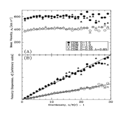
Figure 2: (a) Mean flow $\mu_{v}$ and (b) velocity variance ${\sigma_{v}^{2}}$ as a function of overdensity, $n/{\bar{n}}-1$, for N-body models. These data were computed using $10^{5}$ cells with $r=194\,{\rm km~{}s^{-1}}$ and ${\bar{n}}=1$.

Plots of $\mu_{v}(n,r)$ and $\sigma_{v}(n,r)$ are shown in Figure 2 for the four models. The cell size is $r=194~{}{\rm km~{}s^{-1}}$, corresponding to ${\bar{n}}(r)=1$. All distances are expressed in units of ${\rm km~{}s^{-1}}$. Figure 2 demonstrates three important points: both $\mu_{v}$ and $\sigma_{v}^{2}$ are independent of the shape of the initial power spectrum; $\mu_{v}$ is independent of the local density, while $\sigma_{v}^{2}$ is proportional to the density; and $\mu_{v}$ and $\sigma_{v}^{2}$ have the same strong ${\Omega}$ dependence that ${\langle v^{2}\rangle}$ demonstrated in Figure 1b.

Formally, the power spectrum independence is explained by the derivation of the CVT (see Appendix A). The velocity dispersion depends upon the evolved power spectrum, which is essentially indistinguishable between models (Figure 1). Moreover, any remaining difference between models is encoded in the density distribution function, which is not apparent when density is the dependent variable in Figure 2.

To explore the range over which Eq. (13) is valid, $\mu_{v}$ and ${\sigma_{v}^{2}}$ were calculated over the range of cell sizes $77~{}{\rm km~{}s^{-1}}\leq r\leq 488~{}{\rm km~{}s^{-1}}$, corresponding to $2^{-4}\leq{\bar{n}}(r)\leq 2^{4}$. We obtained the following empirical fit for the mean velocity magnitude

$$\mu_{v}\propto{\Omega}^{1/2}/{\bar{n}}^{\alpha}.$$ (17)

where $\alpha\sim 0.05$. As $\mu_{v}$ already contains the desired ${\Omega}$ dependence, it is convenient to represent $\sigma_{v}^{2}$ in terms of the normalized velocity dispersion $\sigma_{v}^{2}/\mu_{v}^{2}$, with the resulting fit

$$\sigma_{v}^{2}/\mu_{v}^{2}\propto n/{\bar{n}}^{1/3},$$ (18)

which agrees with the theory to within the small factor ${\bar{n}}^{2\alpha}$.

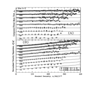
Figure 3: Empirical fits to (a) $\mu_{v}$ and (b) ${\sigma_{v}^{2}}$, as given by Eqs. (17) and (18). The vertical axis has been scaled so that each line of points corresponds to a different cell size. From top to bottom the cell sizes are $r({\rm km~{}s^{-1}})=[488,388,308,244,194,154,122,97,77]$ corresponding to ${\bar{n}}(r)=[2^{4},2^{3},2^{2},2^{1},2^{0},2^{-1},2^{-2},2^{-3},2^{-4}]$. The horizontal axis is in terms of scaled units $n/{\bar{n}}^{1/3}$. The lines indicate the value obtained from the empirical fits.

The quality of the fits can be observed by plotting $\mu_{v}$ and ${\sigma_{v}^{2}}/\mu_{v}^{2}$ against the scaled density ($n/{\bar{n}}^{1/3}$), for each value of $r$. Figure 3a shows the ratio of $\mu_{v}$ to the fitted value computed from Eq. (17) for the ${\Omega}=1$ and ${\Omega}=0.35$ CDM models. Each line of data corresponds to a different value of $r$, and has been offset from the next by one unit. Figure 3b shows a similar plot for the normalized velocity dispersion ${\sigma_{z}^{2}}/\mu_{v}^{2}$. The solid lines are the best fits given by Eq. (18); this has not been divided out. The larger scatter at higher densities and smaller scales is due to the small number of cells contributing to the calculation at these values. The key point to observe from Figure 3a is how well the data points follow the horizontal lines corresponding to their fitted values.

The fits to the data shown in Figure 3 are remarkable, considering that the range includes cells with underdensities ($n/{\bar{n}}-1$) of $-0.8$ on scales of $488~{}{\rm km~{}s^{-1}}$ and cells with overdensities of nearly 200 on scales of $77~{}{\rm km~{}s^{-1}}$. Furthermore, the scaling of $\sigma_{v}^{2}$ is almost exactly that derived from the CVT, indicating that Eq. (13) holds over a large range of scales and densities, even when $\xi(r)\sim 1$.

4 Redshift Dispersion

The purpose of §2 was to theoretically motivate the local density and ${\Omega}$ dependence of ${\sigma_{v}^{2}}$. In §3 the scaling relations in §2 were explored with simple N-body simulations. In addition, §§2 and 3 have introduced the ideas which allow us to describe the main point of this paper—the redshift dispersion.

The formalism we have developed so far cannot be directly applied to observations due to the geometric projection of a six dimensional phase space into a three dimensional redshift survey. The redshift of galaxies represents the only probe, albeit indirect, of the peculiar velocity. Thus, any statistic that desires to take advantage of the properties of ${\sigma_{v}^{2}}$ must be defined with the specific geometry of redshift space in mind. In this section we now describe the redshift dispersion, a statistic with the aim of being readily measurable from volume limited samples taken from redshift surveys and which captures the essence of ${\sigma_{v}^{2}}$.

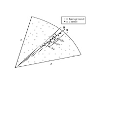
Figure 4: Schematic illustration of the mean redshift, $\mu_{z}$, and the redshift dispersion, ${\sigma_{z}}$, in a pie slice projection of a cluster.

Now let us define quantities analogous to those in §3, but for redshift space. Consider a volume limited sample from a survey out to a maximum redshift of $Z$. Each data point consists of two angular coordinates on the celestial sphere and a redshift. Let us define cells within which to measure density and velocity dispersion in projection on the celestial sphere. The cell $j$ consists of a cone emanating from the origin with solid angle $\pi\theta^{2}$ around the cell center. The number of points in the cone $j$ is $N_{j}$ and is proportional to the projected density on the sky. The mean and the variance of the redshifts in the cone are denoted $u_{j}$ and $\sigma_{j}^{2}$, which are depicted schematically in Figure 4. If ${\cal S}_{n}$ is the set of all cones with $N_{j}=n$, then the average and variance of the redshift as a function of $n$ is

$$\mu_{z}(n,\theta)\equiv{1\over N_{{\cal S}_{n}}}\sum_{j\in{\cal S}_{n}}u_{j}.$$ (19)

and

$$\sigma^{2}_{z}(n,\theta)\equiv{1\over N_{{\cal S}_{n}}}\sum_{j\in{\cal S}_{n}}\sigma^{2}_{j}.$$ (20)

in analogy with Eqs. (15) and (16).

The efficacy with which the ${\sigma_{z}}$ statistic might distinguish between models is examined with the simulations discussed in §3. The simulations were transformed into redshift-space using $Z=5000~{}{\rm km~{}s^{-1}}$, which is equal to one half of the simulation box size. Since the data are periodic, the origin can be placed at any point, allowing multiple perspectives to be drawn from a single simulation. We computed $\sigma_{z}$ for ${\Omega}=1.0$ and ${\Omega}=0.35$ CDM models. The angular cell size was $\theta=1.8\arcdeg$ (${\bar{n}}(\theta)=2$), and the cell centers were computed by creating a pseudo-uniform grid of points across the celestial sphere (Baumgardner & Frederickson 1985). The data have been averaged over 27 different origins regularly distributed throughout the domain, and error bars computed from the standard deviation of this averaging.

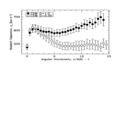
Figure 5: Redshift dispersion, ${\sigma_{z}}$, as a function of angular overdensity for 8000 dark matter particles out to $Z=5000~{}{\rm km~{}s^{-1}}$ averaged over 27 viewpoints. The error bars are the standard deviation of these averages. The angular radius of the cell was $\theta=1.8\arcdeg$, corresponding to ${\bar{n}}=2$.

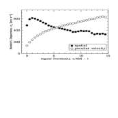
Figure 6: Components of the redshift dispersion, ${\sigma_{z}}$, as a function of angular overdensity for $\Omega=1$ CDM. The spatial component represents the dispersion due to the positions of the particles, while the peculiar velocity component represents the dispersion from the motions of the particles themselves. The measured redshift dispersion is a combination of both components (see Figure 5).

The ${\sigma_{z}}$ curves are plotted in Figure 5. As with the velocity dispersion in Figure 1b, the redshift dispersion shows a strong separation between the low and high ${\Omega}$ models. The differences become apparent at moderate angular over-densities ($\delta\sim 5$). The shape of the curves in Figure 5 is due to the combined spatial and peculiar velocity contributions to ${\sigma_{z}}$, as is illustrated in Figure 6 for the $\Omega=1$ CDM simulation. We know the full six-dimensional position of each galaxy in phase space in the N-body simulation, and thus can separate these two contributions. At low overdensities, ${\sigma_{z}}$ is dominated by the spatial separation of the particles, as is indicated by the solid points in Figure 6; the spatial component scales approximately as $n^{-1/2}$, due to the more tightly bound nature of denser systems. At higher overdensities the peculiar velocity dominates, scaling approximately as $n^{1/2}$, which is consistent with results of §2 and §3. For smaller values of ${\Omega}$ the spatial component behaves the same, but the peculiar velocity component is down by a factor of ${\Omega}^{1/2}$.

These results indicate that the greatest separation in the dispersion between models with different values of ${\Omega}$ will occur in the denser regions; so it is important that we sample many modestly dense regions, which requires a large volume. In addition, to minimize projection effects the sample should not be too deep (i.e., $Z$ not too large). Therefore, to apply the ${\sigma_{z}}$ statistic requires a dense sample over a wide field. If believable simulations of galaxies can be developed it might be possible to constrain models with the same final correlation function by varying $\Omega$ in the simulations and finding the best fit to the observations. For any one point, Figure 5 indicates an error of about 0.15 in $\Omega$. Using many points along the curve, the errors may be small enough to significantly constrain the value of $\Omega$.

The current redshift surveys do not have enough data to attempt such a comparison. To get the level of separation shown in Figure 5 required ${\cal O}(10^{4})$ particles. We have calculated $\sigma_{z}$ from the IRAS 1.2 Jansky survey (Fisher et al. (1995)), but a volume-limited sample taken from this survey contains only 800 galaxies at best. The error bars from an 800 point sample in the simulations were too large to be able to distinguish between high and low ${\Omega}$ models.

Fortunately, a substantial increase in the amount of data available will be brought about by the Sloan Digital Sky Survey (SDSS). The SDSS will obtain spectra and measure the redshifts of the $10^{6}$ galaxies down to $r^{\prime}\sim 18$ (Gunn & Weinberg (1995)). We can estimate the size of a volume-limited sample taken from the SDSS using the Schechter luminosity function $\phi_{s}$ fitted to the Stromlo-APM survey (Loveday et al. (1992))

$$\phi_{s}(L)dL=\phi^{\star}y^{\alpha}e^{-y}dy,~{}~{}~{}y=L/L^{\star},$$ (21)

where $\phi^{\star}\simeq 1.4\times 10^{-8}\,{\rm km^{-3}\,s^{3}}$, $M^{\star}\simeq-19.5$, and $\alpha\simeq-0.97$ are parameters obtained from the fit. The number of galaxies in a given volume, $V$, brighter than $L_{0}$, $N(V,L_{0})$, can be computed by integrating the luminosity function

$$N(V,L_{0})=V\int_{L_{0}}^{\infty}\phi(L)dL=V\int_{y_{0}}^{\infty}\phi^{\star}y^{\alpha}e^{-y}dy=V\phi^{\star}\Gamma(\alpha+1,y_{0}),$$ (22)

where $y_{0}=L_{0}/L^{\star}$. For a volume limited survey, $L_{0}$ is the luminosity an object would have if it had an apparent magnitude $m_{0}$ and was located at the volume edge $Z$ ($H_{0}=100\,{\rm km~{}s^{-1}}\,{\rm Mpc}^{-1}$). From this definition it follows that

$$y_{0}=Z^{2}_{{\rm km~{}s^{-1}}}\,10^{0.4(M^{\star}-m_{0}+15)},$$ (23)

where $m_{0}$ is the apparent magnitude limit of the survey. The Stromlo-APM survey was taken in the $b_{j}$ band, while the Sloan will use the $r^{\prime}$ band. The two can be equated by the approximate relation $b_{j}\sim r^{\prime}+1$. However, we set $m_{0}=18.7$ which gives a better value for the estimated total number of galaxies in the survey ($10^{6}$). Inserting $Z=5000\,{\rm km~{}s^{-1}}$ into Eq. (23) gives $y_{0}\approx 0.013$. Setting $V_{SDSS}=\pi Z^{3}/3$ results in $N_{SDSS}\approx 7000$. This number might in fact be appreciably larger if there are many more faint galaxies than Eq. (22) implies, and has been suggested by recent surveys for low-surface brightness galaxies (cf., Dalcanton (1995)). However, these galaxies are unlikely to have redshifts measured as part of the SDSS.

One could substantially increase the number of galaxies in a volume-limited survey of fixed depth by dropping the requirement that it include the origin. Figure 7 plots the expected number of galaxies in a series of volume limited shells for SDSS and shows that a redshift shell between $25,000\,{\rm km~{}s^{-1}}$ and $30,000\,{\rm km~{}s^{-1}}$ would include almost $10^{5}$ galaxies!

Ultimately, applying the redshift dispersion statistic to the SDSS could provide many data points for comparing with simulations and perhaps constraining $\Omega$. The ${\sigma_{z}}$ curves can be evaluated for many angular sizes and redshift shells for both the SDSS and for several next generation, high resolution, N-body/hydrodynamic simulations with different values of ${\Omega}$. Since the number of estimated objects in the SDSS is the same order or more as the simulations shown in Figure 5, one might expect to obtain an equivalent separation between models for each value. It should be interesting to compare ${\sigma_{z}}$ measured in different simulations with the SDSS as a function of $n$, $\theta$ and shell geometry.

5 Conclusions

Our goal has been to present a new statistic—the redshift dispersion (${\sigma_{z}}$)—that is sensitive to ${\Omega}$ and is well suited for comparing real and simulated volume limited samples from redshift surveys. Given the proper data, ${\sigma_{z}}$ is easy to compute and can be applied on many scales without applying arbitrary assumptions. We have used low resolution simulations, which are sufficient for our motivational purposes, to do a simple exploration of ${\sigma_{z}}$, which suggests that applying it to the SDSS may be worthwhile. In addition, with the right simulations, it might be possible to constrain ${\Omega}$ in models where the simulations match the observed final correlation function.

We have shown that the pairwise velocity dispersion is intrinsically related to the local density and ${\Omega}$. In §2 and Appendix A it is shown that the CVT holds for each particle in a system and subsequently for any subset of particles, if we are careful to define the velocity dispersion and correlation function for these subsets appropriately. The density dependence of the velocity dispersion can be extracted by looking at subsets of particles of a given local density (see Eq. 13). Knowing how ${\sigma_{v}^{2}}$ depends upon the local density gives an indication as to why the standard approach of averaging ${\langle v^{2}\rangle}$ over all densities is highly sensitive to the presence of rare density peaks. Exploring Eq. (13) with N-body simulations of several cosmological models indicates that it holds over a wide range of length scales, $77~{}{\rm km~{}s^{-1}}\leq r\leq 488~{}{\rm km~{}s^{-1}}$. Our redshift dispersion statistic is simply the redshift-space analog of the quantity ${\sigma_{v}}$.

We have treated our galaxies as equal mass particles containing all the mass, ignoring the hypothesized global stochastic mapping from the dark matter mass and velocity distribution to the distribution of galaxies (i.e. the mass and velocity bias functions), which may differ among the models. A more general treatment would estimate the mass and velocity bias in each model and normalize the models such that the galaxy correlations, not the dark matter correlations, are similar. At best, reliable estimates of these bias functions await the next generation of simulations where galaxies can be resolved within statistically meaningful volumes. However, there are several arguments as to why the differences in the biases between models may not strongly affect our work. First, the initial power spectra of currently favored hierarchical models all have similar slopes on galaxy formation scales. Hence, the initial conditions of galaxy formation—and the resulting bias—may be similar. In addition, the HDM model, which has a very different initial power spectrum, has a similar final correlation function, which suggests that the final power on small scales is dominated by non-linear processes which erase initial differences. Any velocity bias which arises through dynamical friction should be similar for models evolved to similar clustering levels. If velocity bias is related to galaxy formation sites preferentially near potential wells, then velocity bias could depend on mass density and the efficacy of this measure could be diminished. However, both types of bias appear to be strong only in the most non-linear regions ($\delta\gtrsim 200$) (Summers, Davis, & Evrard (1995)), while our study focuses on the mildly non-linear regimes ($\delta\sim 10$).

High resolution, hydrodynamic simulations that include detailed galaxy formation should improve our understanding of bias and how it changes from model to model. Intuitively, any bias, by eliminating objects in the underdense regions, should have the overall effect of shifting the data points in Figure 5 to the left. Higher resolution will also incorporate the interactions of dark matter halos, which may significantly effect the three point correlation function on galaxy scales (see Bartlett & Blanchard (1996)). All of these effects indicate more detailed simulations, beyond what is currently available, may be necessary for the actual application of the redshift dispersion.

The next logical step is to attempt to apply ${\sigma_{z}}$ to denser redshift surveys than the IRAS 1.2 Jansky survey. In the mean time, additional studies on larger volume, higher resolution N-body simulations would be useful, but perhaps overkill until a suitable redshift survey becomes available. Also, it is not clear that using dark matter halos without the proper means for identifying galaxies would add to these results. Further exploration should also be done on a wide variety of survey geometries. Here, we only looked at a single small sphere. It is quite possible that a larger sphere or a shell might be the optimal shape to balance the tradeoff between high density and large numbers of clusters that make ${\sigma_{z}}$ work best.

Appendix A Cosmic Virial Theorem

In §2 we showed that the CVT applied to sets of particles provided it holds for individual particles. To prove the latter result we return to Peebles’ original derivation (see P76). Davis & Peebles (1977) later rederived the Cosmic Virial Theorem by placing it in the context of the BBGKY hierarchy. We choose to use the earlier approach because of its simpler, more intuitive nature. The essential derivation is still that found in P76, but a few minor modifications have been added to elaborate key steps in the derivation.

The derivation of the CVT proceeds in the following manner. First, an equation linking the velocity, acceleration, and correlation function of a general particle system is obtained from the conservation of phase space density. Second, the accelerations are linked through gravity to the two and three point correlation functions. Third, the assumptions of a cosmological system are applied to the general particle equation to obtain the scaling between the velocity dispersion and the density. The key modification that we have made in order to show that this result applies for individual particles in the system is to replace the entire phase space with the phase space of a single particle.

A.1 Phase Space Conservation

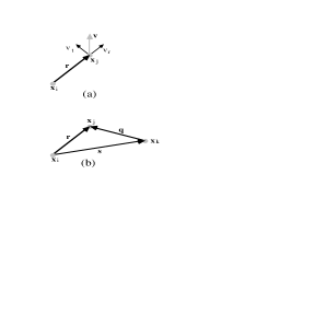
Figure 8: Schematic drawings depicting positions and velocities of (a) two particle and (b) three particle systems used to derive the Cosmic Virial Theorem.

To start, consider a system of particles with the position, velocity, and acceleration of the $i$th particle given by ${\bf{x}}_{i}$, ${\bf{v}}_{i}$, and ${\bf{a}}_{i}$. Strictly speaking, these are not phase space variables, but represent a three-dimensional single-particle distribution and its evolution in time. Now consider any two particles $i$ and $j$ having relative position, velocity, and acceleration: ${\bf{r}}={\bf{x}}_{j}-{\bf{x}}_{i}$, ${\bf{v}}={\bf{v}}_{j}-{\bf{v}}_{i}$, ${\bf{a}}={\bf{a}}_{j}-{\bf{a}}_{i}$, as shown in Figure 8a. The rate of change in the distance, $r$, between the two particles obeys

$${\dot{r}}=v_{r}={{\bf{r}}\!\cdot\!{\bf{v}}}/r,$$ (A1)

and the acceleration

$${\ddot{r}}=({{\bf{r}}\!\cdot\!{\bf{a}}}+v^{2}-({{\bf{r}}\!\cdot\!{\bf{v}}}/r)^{2})/r=({{\bf{r}}\!\cdot\!{\bf{a}}}+v_{t}^{2})/r,$$ (A2)

where $v^{2}=v_{r}^{2}+v_{t}^{2}$. For a sufficiently large system, the number of particles found in a volume of phase space centered on the $i$th particle is $dN_{{i\!\times\!{\cal P}}}=f_{{i\!\times\!{\cal P}}}(r,{\dot{r}},{\ddot{r}})drd{\dot{r}}d{\ddot{r}}$, where $f_{{i\!\times\!{\cal P}}}$ is the phase space density of all pairs connected to the particle $i$. The function $f_{{i\!\times\!{\cal P}}}$ is related to the two point correlation function by

$$dr\int d{\dot{r}}d{\ddot{r}}f_{{i\!\times\!{\cal P}}}={\bar{\nu}}(1+\xi_{{i\!\times\!{\cal P}}})4\pi r^{2}dr,$$ (A3)

where ${\bar{\nu}}$ is the mean number density and $\xi_{{i\!\times\!{\cal P}}}=\xi_{{i\!\times\!{\cal P}}}(r)$ is the isotropic two point correlation function of the $i$th particle, which is defined with respect to the joint probability $dP_{2}=dV_{i}dV_{j}{\bar{\nu}}^{2}(1+\xi_{{i\!\times\!{\cal P}}})$.

For convenience, we now explicitly drop the subscript ${i\!\times\!{\cal P}}$ notation: $f_{{i\!\times\!{\cal P}}}\rightarrow f$, $N_{{i\!\times\!{\cal P}}}\rightarrow N$, and $\xi_{{i\!\times\!{\cal P}}}\rightarrow\xi$. It should be understood that all these quantities are relative to the $i$th particle, including the velocities and accelerations.

Having defined the particle system and the phase space density, $f$, it is now possible to look at the time evolution of the particle within the system. The integral of $f$ links it to $\xi$ giving the total number of particles with separation between $r$ and $r+{\delta r}$. The number of particles with separation less than $r$ is

$$N(r,t)=\int_{0}^{r}dr\int d{\dot{r}}d{\ddot{r}}f.$$ (A4)

At some later time ${\delta t}$ there exists a ${\delta r}$ such that

$$N(r,t)=N(r+{\delta r},t+{\delta t}).$$ (A5)

Without loss of generality, we could have just as well started at the point $N(r-{\delta r},t)$, and chosen ${\delta t}$ and ${\delta r}$ to satisfy

$$N(r-{\delta r},t)=N(r,t+{\delta t}),$$ (A6)

which allows us to expand around $r$ and $t$. Subtracting $N(r,t)$ from the above expression, we have

$$-[N(r,t)-N(r-{\delta r},t)]=N(r,t+{\delta t})-N(r,t).$$ (A7)

The right side can be readily expanded in powers of ${\delta t}$ and is simply ${\delta t}{\dot{N}}+{\textstyle\frac{1}{2}}{\delta t}^{2}{\ddot{N}}$. Likewise, from the definition of $N(r,t)$ the left side is given by

$$-[N(r,t)-N(r-{\delta r},t)]=-\int d{\dot{r}}d{\ddot{r}}\int_{r-{\delta r}}^{r}drf.$$ (A8)

The Taylor expansion of the integral gives

$$\int_{r}^{r^{\prime}}drf \simeq {\textstyle\frac{1}{2}}{\delta r}[f(r)+f(r-{\delta r})]$$ (A9)

$$\simeq {\delta r}f-{\textstyle\frac{1}{2}}{\delta r}^{2}{\partial_{r}}f$$

$$\simeq {\delta t}{\dot{r}}f+{\textstyle\frac{1}{2}}{\delta t}^{2}({\ddot{r}}f-{\dot{r}}^{2}{\partial_{r}}f),$$

where the last step made use of the following expansion for ${\delta r}$

$${\delta r}={\delta t}{\dot{r}}+{\textstyle\frac{1}{2}}{\delta t}^{2}{\ddot{r}}+\ldots,$$ (A10)

which is valid for fixed ${\dot{r}}$ and ${\ddot{r}}$.

Matching powers of ${\delta t}$ gives an expression for ${\ddot{N}}$

$${\ddot{N}} = -\int d{\dot{r}}d{\ddot{r}}({\ddot{r}}-{\dot{r}}^{2}{\partial_{r}})f$$ (A11)

$$= -\int d{\dot{r}}d{\ddot{r}}\,{\ddot{r}}f+{\partial_{r}}\int d{\dot{r}}d{\ddot{r}}\,{\dot{r}}^{2}f$$

$$= -{\bar{\nu}}4\pi[r^{2}{(1+\xi)}{\langle{\ddot{r}}\rangle}-{\partial_{r}}(r^{2}{(1+\xi)}{\langle{\dot{r}}^{2}\rangle})],$$

where we have used ${\partial_{r}}{\dot{r}}=0$, but ${\partial_{r}}{\langle{\dot{r}}^{2}\rangle}\neq 0$. The time derivative of $N$ can be written

$${\ddot{N}}=4\pi{\bar{\nu}}{\partial_{t}^{2}}\int_{0}^{r}dr\,r^{2}{(1+\xi)}=4\pi{\bar{\nu}}\int_{0}^{r}dr\,r^{2}{\ddot{\xi}},$$ (A12)

which is combined with the previous expression to give

$${\ddot{N}}\propto{\partial_{r}}[r^{2}{(1+\xi)}{\langle{\dot{r}}^{2}\rangle}]-r^{2}{(1+\xi)}{\langle{\ddot{r}}\rangle}=\int_{0}^{r}dr\,r^{2}{\ddot{\xi}}.$$ (A13)

Substituting in the expressions for ${\dot{r}}$ and ${\ddot{r}}$, and expanding the $r$ derivative results in the general equation derived in P76

$$r{\partial_{r}}[{(1+\xi)}{\langle v_{r}^{2}\rangle}]+{(1+\xi)}{\langle 2v_{r}^{2}-v_{t}^{2}\rangle}={(1+\xi)}{\langle{{\bf{r}}\!\cdot\!{\bf{a}}}\rangle}+r^{-1}\int_{0}^{r}dr\,r^{2}{\ddot{\xi}}.$$ (A14)

This equation represents the conservation of phase space for a single particle in a system, and is true for any particle in the system with a well defined phase space density and an isotropic two-point correlation function.

A.2 Gravitating Particles

For gravitationally interacting particles, the acceleration term is simply ${\langle{{\bf{r}}\!\cdot\!{\bf{a}}}\rangle}={\langle{\bf{r}}\!\cdot\!({\bf{g}}_{j}-{\bf{g}}_{i})\rangle}$, where

$${\bf{g}}_{i}=G\sum_{j}m_{j}\frac{{\bf{x}}_{j}-{\bf{x}}_{i}}{|{\bf{x}}_{j}-{\bf{x}}_{i}|^{3}}.$$ (A15)

When averaging over phase space, ${\bf{g}}_{i}$ can be written in terms of the two and three point correlation functions, which requires considering a third particle at ${\bf{x}}_{k}$ (see Figure 8b). The average force on $i$ is the force from $j$ plus the force due to $k$ weighted by the conditional probability of the third particle being located at ${\bf{s}}$

$${\langle{\bf{g}}_{i}\rangle} = \frac{Gm{\bf{r}}}{r^{3}}+Gm\int\frac{{\bf{s}}}{s^{3}}\frac{dP_{3}}{dP_{2}}$$ (A16)

$$= \frac{Gm{\bf{r}}}{r^{3}}+\frac{G\rho}{1+\xi}\int d^{3}{\bf{s}}\frac{{\bf{s}}}{s^{3}}[1+\xi(r)+\xi(s)+\xi(q)+\zeta(r,s,q)]$$

where $m$ is the average mass per particle and the three point correlation function $\zeta$ is defined by the probability

$$dP_{3}=dV_{i}dV_{j}dV_{k}{\bar{\nu}}^{3}[1+\xi(r)+\xi(s)+\xi(q)+\zeta(r,s,q)].$$ (A17)

The first, second and third terms in the brackets integrate to zero by isotropy leaving

$${\langle{\bf{g}}_{i}\rangle}=\frac{Gm{\bf{r}}}{r^{3}}+\frac{G\rho}{1+\xi}\int d^{3}{\bf{s}}\frac{{\bf{s}}}{s^{3}}[\xi(q)+\zeta(r,s,q)].$$ (A18)

Likewise, the force on $j$ is

$${\langle{\bf{g}}_{j}\rangle}=-\frac{Gm{\bf{r}}}{r^{3}}-\frac{G\rho}{1+\xi}\int d^{3}{\bf{q}}\frac{{\bf{q}}}{q^{3}}[\xi(s)+\zeta(r,q,s)].$$ (A19)

Because $\zeta(r,s,q)=\zeta(r,q,s)$, the average of the total force is

$${\langle{\bf{r}}\!\cdot\!({\bf{g}}_{j}-{\bf{g}}_{i})\rangle}=-\frac{2Gm}{r}-\frac{2G\rho}{1+\xi}\int d^{3}{\bf{s}}\frac{{{\bf{r}}\!\cdot\!{\bf{s}}}}{s^{3}}[\xi(q)+\zeta(r,s,q)].$$ (A20)

A.3 Cosmological Scalings

To obtain the scaling of the velocity dispersion we apply various approximations that are consistent with a cosmological model. First, we consider the situation where the correlation function is assumed to be stationary in comparison to the motions of the particles, i.e., the time scale for changes in $\xi$ is much greater than the crossing time $r/{\langle v_{r}^{2}\rangle}^{1/2}\rightarrow{\ddot{\xi}}=0$. In addition, ${\bf{v}}$ is randomly oriented so that ${\langle v^{2}\rangle}/3\simeq{\langle v_{t}^{2}\rangle}/2\simeq{\langle v_{r}^{2}\rangle}$, and ${\langle 2v_{r}^{2}-v_{t}^{2}\rangle}=0$. These assumptions eliminate two terms from Eq. (A14). Combining with Eq. (A20) gives

$$r{\partial_{r}}[{(1+\xi)}{\langle v^{2}\rangle}]=-\frac{6Gm{(1+\xi)}}{r}-6G\rho\int d^{3}{\bf{s}}\frac{{{\bf{r}}\!\cdot\!{\bf{s}}}}{s^{3}}[\xi(q)+\zeta(r,s,q)].$$ (A21)

The next step is to evaluate the integrals on the right. At this point we impose a model for $\xi$ and $\zeta$. Observations indicate that the correlation functions are well modeled by power laws of the form

$$\xi(r)=\left(\frac{r_{0}}{r}\right)^{\gamma},~{}~{}~{}\gamma=1.77,~{}~{}~{}r_{0}=5.4{h^{-1}{\rm Mpc}}$$ (A22)

and,

$$\zeta(r,s,q)=Q[\xi(r)\xi(s)+\xi(r)\xi(q)+\xi(s)\xi(q)],~{}~{}~{}Q\simeq 1.0.$$ (A23)

Using these relationships, the first integral can be solved with the following identities ${{\bf{r}}\!\cdot\!{\bf{s}}}=rs\cos\theta$, and $q^{2}=r^{2}-2sr\cos\theta+s^{2}$, and by noting that in spherical coordinates $d^{3}{\bf{s}}=s^{2}ds\sin\theta d\theta d\phi$

$$\int d^{3}{\bf{s}}\frac{{{\bf{r}}\!\cdot\!{\bf{s}}}}{s^{3}}\xi(q) = \int s^{2}ds\sin\theta\,d\theta d\phi\frac{rs\cos\theta}{s^{3}}\xi(q)$$ (A24)

$$= 2\pi\int ds\,d\theta\,r\cos\theta\sin\theta\,\xi((r^{2}-2sr\cos\theta+s^{2})^{1/2})$$

$$= 2\pi r^{2}\int dy\,d\theta\cos\theta\sin\theta\,\xi((r^{2}-2yr^{2}\cos\theta+y^{2}r^{2})^{1/2})$$

$$= 2\pi\xi r^{2}\int_{0}^{\infty}dy\int_{0}^{\pi}\frac{d\theta\cos\theta\sin\theta}{(1-2y\cos\theta+y^{2})^{\gamma/2}}$$

$$= \frac{2\pi\xi r^{2}J_{\gamma}}{(2-\gamma)(4-\gamma)}.$$

where $J_{\gamma}=\int_{0}^{\infty}dyI_{\gamma}(y)/y^{2}$, $y=s/r$, and

$$I_{\gamma}(y)=(y+1)^{2-\gamma}\{1-(2-\gamma)y+y^{2}\}-|y-1|^{2-\gamma}\{1+(2-\gamma)y+y^{2}\}$$ (A25)

For the second integral, we obtain a similar result

$$\int d^{3}{\bf{s}}\frac{{{\bf{r}}\!\cdot\!{\bf{s}}}}{s^{3}}\zeta(r,s,q) = \int d^{3}{\bf{s}}\frac{{{\bf{r}}\!\cdot\!{\bf{s}}}}{s^{3}}Q[\xi(r)\xi(s)+\xi(r)\xi(q)+\xi(s)\xi(q)]$$ (A26)

$$= Q\int d^{3}{\bf{s}}\frac{{{\bf{r}}\!\cdot\!{\bf{s}}}}{s^{3}}\xi(q)[\xi(r)+\xi(s)]$$

$$= \frac{2\pi Q\xi^{2}r^{2}M_{\gamma}}{(2-\gamma)(4-\gamma)},$$

where $M_{\gamma}=\int_{0}^{\infty}dy(1+y^{-\gamma})I_{\gamma}(y)/y^{2}$. For our purposes, it is sufficient to know that $J_{1.8}$ and $M_{1.8}$ are of order unity. Inserting the above results into Eq. (A22) gives

$$r{\partial_{r}}[{(1+\xi)}{\langle v^{2}\rangle}]=-\frac{6Gm{(1+\xi)}}{r}-\frac{12\pi G\rho\xi r^{2}J_{\gamma}}{(2-\gamma)(4-\gamma)}-\frac{12\pi G\rho Q\xi^{2}r^{2}M_{\gamma}}{(2-\gamma)(4-\gamma)}.$$ (A27)

Finally, let $\xi\gg 1$. Dividing through by $r$, and integrating from $r$ to $\infty$ and dividing again by $\xi$, gives an equation for the velocity dispersion

$${\langle v^{2}\rangle}(r)=\frac{6Gm}{(\gamma+1)r}+\frac{12\pi G\rho r^{2}J_{\gamma}}{(2-\gamma)^{2}(4-\gamma)}+\frac{6\pi G\rho Q\xi(r)r^{2}M_{\gamma}}{(\gamma-1)(2-\gamma)(4-\gamma)}$$ (A28)

For small $r$ the third term dominates the second. The first term is negligible in the limit that $m$ is very small, i.e., that the mass is divided up into many tiny individual particles. Thus the third term dominates, leaving the classic result

$${\langle v^{2}\rangle}(r)=\frac{6\pi G\rho Q\xi(r)r^{2}M_{\gamma}}{(\gamma-1)(2-\gamma)(4-\gamma)}.$$ (A29)

Using the definition $H^{2}=8\pi G\rho/3{\Omega}$, we can rewrite the above expression as

$${\langle v^{2}\rangle}(r)=\frac{9{\Omega}Q(Hr)^{2}\xi(r)M_{\gamma}}{4(\gamma-1)(2-\gamma)(4-\gamma)}.$$ (A30)

which, if we return to the earlier notation (measuring distances in terms of velocity $Hr$) gives the expression quoted in Eq. (4) of §2

$${\langle v_{{i\!\times\!{\cal P}}}^{2}\rangle}(r)\propto{\Omega}\xi_{{i\!\times\!{\cal P}}}(r)r^{2},$$ (A31)

with a proportionality constant

$$C_{1}=\frac{9{\Omega}QM_{\gamma}}{4(\gamma-1)(2-\gamma)(4-\gamma)}.$$ (A32)

Figure 7: Estimated number of galaxies in each volume limited shell of the SDSS.

References

- Bartlett & Blanchard (1996) Bartlett, J., & Blanchard, A. 1996, A&A, 307, 1
- Baumgardner & Frederickson (1985) Baumgardner, J.R., & Frederickson, P.O. 1985, SIAM J. Numer. Anal., 22, 1107
- Bertschinger & Gelb (1991) Bertschinger, E., & Gelb, J. 1991, Computers in Physics, 5, 164
- Brieu, Summers, & Ostriker (1995) Brieu, P.P., Summers, F J, & Ostriker, J.P. 1995, ApJ, 453, 566
- Brown & Peebles (1987) Brown, M., & Peebles, P.J.E. 1987, ApJ, 317, 588
- Burstein (1990) Burstein, D. 1990, Rep. Prog. Phys., 53, 421
- Couchman & Carlberg (1992) Couchman, H., & Carlberg, R. 1992, ApJ, 389, 453
- Dalcanton (1995) Dalcanton, J., 1995, Ph.D. Thesis, Princeton University
- Davis & Peebles (1977) Davis, M., & Peebles, P.J.E. 1977, ApJS, 34, 425
- Davis & Peebles (1983) Davis, M., & Peebles, P.J.E. 1983, ApJ, 267, 465
- Efstathiou, Bond, & White (1992) Efstathiou, G., Bond, J. R., & White, S. D. M. 1992, MNRAS, 258, 1
- Efstathiou et al. (1985) Efstathiou, G., Davis, M., White, S.D.M., & Frenk, C.S. 1985, ApJS, 57, 241
- Efstathiou et al. (1988) Efstathiou, G., Frenk, C.S., White, S.D.M. & Davis, M. 1988, MNRAS, 235, 715
- Evrard, Summers, & Davis (1994) Evrard, A. E., Summers, F J, & Davis, M. 1994, ApJ, 422, 11
- Fisher et al. (1994) Fisher, K.B., Davis, M., Strauss, M.A., Yahil, A., & Huchra, J. 1994, MNRAS, 267, 927
- Fisher et al. (1995) Fisher, K.B., Huchra, J., Strauss, M.A., Davis, M., Yahil, A., & Schlegel, D. 1995, ApJS, 100, 69
- Gelb & Bertschinger (1994) Gelb, J., & Bertschinger, E. 1994, ApJ, 436, 491
- Górski et al. (1995) Górski, K. M., Ratra, B., Sugiyama, N., & Banday, A. J. 1995, ApJ, 444, L65
- Gunn & Weinberg (1995) Gunn, J.E., & Weinberg, D.H. 1995, in S.J. Maddox and A. Aragón-Salamanca eds, Wide-Field Spectroscopy and the Distant Universe (Singapore: World Scientific), 3
- Guzzo et al. (1996) Guzzo, L., Fisher K.B., Strauss, M.A., Giovanelli, R., & Haynes, M.P. 1996, Astroph. Lett. & Comm., 33, 231
- Hockney & Eastwood (1981) Hockney, R.W., & Eastwood, J.W. 1981, Computer Simulation Using Particles (New York: McGraw–Hill)
- Holtzman (1989) Holtzman, J. 1989, ApJS, 71, 1
- Loveday et al. (1996) Loveday, J., Efstathiou, G., Maddox, S. J., & Peterson, B.A. 1996, ApJ, 468, L1
- Loveday et al. (1992) Loveday, J., Peterson, B.A., Efstathiou, G., & Maddox, S. J. 1992, ApJ, 390, 338
- Marzke et al. (1995) Marzke, R.O., Geller, M.J., da Costa, L.N., & Huchra, J.P. 1995, AJ, 110, 477
- Mo, Jing, & Börner (1993) Mo, H.J., Jing, Y.P., & Börner, G. 1993, MNRAS, 264, 825
- Okumura et al. (1993) Okumura, S. K., et al. 1993, PASJ, 45, 329
- (28) Peebles, P.J.E. 1976a, Ap&SS, 45, 3 (P76)
- (29) Peebles, P.J.E. 1976b, ApJ, 205, L109
- Peebles (1980) Peebles, P.J.E. 1980, The Large-Scale Structure of the Universe (Princeton: Princeton University Press)
- Sandage (1986) Sandage, A. 1986, ApJ, 307, 1
- Somerville, Davis, & Primack (1997) Somerville, R.S., Davis, M., & Primack, J.R. 1997, ApJ, 479, 616
- Stompor, Górski, & Banday (1995) Stompor, R., Górski, K. M., & Banday, A. J. 1995, MNRAS, 277, 1225
- Strauss, Cen, & Ostriker (1993) Strauss, M.A., Cen, R.Y., & Ostriker, J.P. 1993, ApJ, 408, 389
- Strauss & Willick (1995) Strauss, M.A., & Willick, J.A. 1995, Phys. Rep., 261, 271
- Summers, Davis, & Evrard (1995) Summers, F J, Davis, M., & Evrard, A. E. 1995, ApJ, 454, 1
- Willick et al. (1997) Willick, J.A., Strauss, M.A., Dekel, A., & Kolatt, T. 1997, ApJ, in press (astro-ph/9612240)
- Zurek et al. (1994) Zurek, W.H., Quinn, P.J., Salmon, J.K., & Warren, M.S., 1994, ApJ, 431, 559