[
Accurate determination of inflationary perturbations
Abstract
We use a numerical code for accurate computation of the amplitude of linear density perturbations and gravitational waves generated by single-field inflation models to study the accuracy of existing analytic results based on the slow-roll approximation. We use our code to calculate the coefficient of an expansion about the exact analytic result for power-law inflation; this generates a fitting function which can be applied to all inflationary models to obtain extremely accurate results. In the appropriate limit our results confirm the Stewart–Lyth analytic second-order calculation, and we find that their results are very accurate for inflationary models favoured by current observational constraints.
pacs:
PACS numbers: 98.80.Cq SUSSEX-AST 96/7-4, astro-ph/9607096]
I Introduction
In anticipation of a near-future launch of a satellite capable of measuring microwave background anisotropies to an accuracy of a few percent or better across a wide range of angular scales [1], attention has recently been directed towards obtaining highly accurate predictions of the anisotropies for given cosmological models. It is now possible for fast and extremely accurate calculations, good to a percent or so, of the radiation anisotropy power spectrum to be made [2], given the spectrum of density perturbations in the universe.
A very promising theory for the generation of such perturbations is cosmological inflation [3], wherein the universe experiences a period of accelerated expansion in its very early stages. In order to take advantage of the great observational accuracy anticipated, it is desirable to make as accurate calculations as possible of the perturbations which inflation produces. Such accurate calculations are the focus of this paper.
When density perturbations from inflation were first discussed [4, 5], the result was typically quoted along the lines of
| (1) |
where the right hand side is evaluated as the scale crosses outside the Hubble radius during inflation, and the left hand side as it crosses back inside after inflation. Here is the Hubble parameter and is the scalar field driving inflation. That the result was given only approximately was through a combination of the calculations not being completely accurate, and the lack of a precise definition of the left hand side of this equation, usually described as the fractional density perturbation when a scale enters the horizon. Fairly quickly, however, a precise definition of this quantity was made and the coefficient computed [5, 6]. In more modern notation, defined later in this paper, the result is
| (2) |
The right hand side is evaluated as before, but now the left hand side, giving the spectrum of the curvature perturbation , holds at any time when the scale is much larger than the Hubble radius, the curvature perturbation being constant in that limit. The uncertainty in the calculation was then due to the fact that its derivation depended on the inflationary slow-roll approximation; for some models this can be extraordinarily good but in many the associated error would be expected to be order of ten percent or greater.
The next development was the presentation of a precise calculation in the case of power-law inflation, by Lyth and Stewart [7]. The analogous but simpler exact calculation for the gravitational wave amplitude in this model was made much earlier by Abbott and Wise [8]. The precise calculation allowed a direct evaluation of the uncertainty induced in these models by use of the slow-roll approximation. Stewart and Lyth then went on to use this exact result to analytically compute the next-order slow-roll correction to the standard formula [9]. In principle, one would like to carry out the expansion about any power-law inflation model, but in practice analytic considerations required a restriction to an expansion about power-law inflation models which were themselves near the de Sitter limit. One should therefore regard that calculation as a slow-roll expansion rather than an expansion about the power-law inflation solution.
A slightly different kind of calculation, which we shall not further discuss, can be done in the case where the potential takes the form , in the limit where dominates. For the inverted harmonic oscillator (natural inflation) this was carried out by Stewart and Lyth [9] and for positive mass (hybrid inflation) an analysis was performed by García-Bellido and Wands [10]. There a much more accurate calculation can be made than the slow-roll one, even if the mass is quite large, but again this calculation is restricted to this particular class of models.
For most models of inflation, the Stewart–Lyth calculation should give extremely accurate predictions. In this paper, we use a numerical code to test their accuracy against exact results, finding that the agreement is extremely good. We then use our code as the basis for an even more accurate scheme, using it to carry out an expansion about any power-law inflation solution, even those far from the de Sitter limit. This gives a highly accurate fitting function for the amplitude in any inflation model, by regarding them as expansions about the ‘nearest’ power-law inflation model.
II The Density Perturbation Calculation
A Evolution of perturbations
Standard calculations of the density perturbation amplitude from inflationary models rely on two separate types of assumption, linear perturbation theory and the slow-roll approximation for the inflationary evolution of the background space-time. The first of these approximations is considerably better than the second, since we know from COBE that the amplitude of perturbations is about one part in , and we shall use it throughout.
The slow-roll approximation is typically much less good, because in order for inflation to end the slow-roll conditions must break. While for some inflationary models it is extremely good, it is perfectly possible for it to fail by ten percent or more in others, including some still permitted by present observational constraints. Hence our aim in this paper to make calculations which do not depend on the slow-roll approximation, and also to provide more accurate approximations for the density perturbations based on a version of the slow-roll expansion.
Before proceeding to the calculation, let us highlight that we are limiting discussion to inflation driven by a single, canonically normalized, scalar field in Einstein gravity. While this looks like quite a restrictive assumption, is is actually fairly general, in the sense that almost any extended theory of gravity, such as a higher-order or scalar–tensor theory, can be rewritten as Einstein gravity via a conformal transformation. Further, models with more than one scalar field often effectively only have a single degree of freedom, with fluctuations transverse to the evolving field having their fluctuations suppressed by a large effective mass; this situation occurs, for example, when extended inflation is conformally transformed to give power-law inflation [11], and also in the hybrid inflation model [12]. However, our calculations will not be valid in any theory in which fluctuations in more than one field are important, and it is possible to construct situations where this is the case [13].
Our analysis is based on the formalism devised by Stewart and Lyth [9] to carry out a second-order analytic calculation. We shall not reproduce the derivation of the equations here, instead simply reproducing the important ones.***An expanded discussion of the Stewart–Lyth calculation is given in Ref. [14]. With the usual notation of for scale factor, for Hubble parameter, for the inflationary scalar field and overdot as derivative with respect to cosmic time, they introduce a new quantity defined by
| (3) |
The quantity one desires to calculate is the curvature perturbation , defined as in Ref. [9]. It is convenient to define a related quantity , defined by
| (4) |
which is a gauge invariant potential [15].
A Fourier expansion of into comoving modes is carried out, and these can be shown to obey the remarkably simple equation [16, 15, 9]
| (5) |
where is the conformal time defined by and is the modulus of the wavenumber. Defining the spectrum of the curvature perturbation in the standard way as
| (6) |
yields
| (7) |
which statistical isotropy permits to depend only on the modulus . From here on, we’ll label modes by their modulus rather than their full wavenumber.
During inflation, a comoving scale evolves from well inside the Hubble radius to well outside it. Canonical quantization of demands that in the initial state, where the expansion can be ignored, it approaches the standard flat space result [9]
| (8) |
In the opposite regime, where can be ignored in Eq. (5), the equation can be integrated directly to give
| (9) |
implying that the spectrum approaches a constant in this regime.
Notice that the entire quantum part of this calculation is in the normalization at large , which is the Minkowski space limit. Once that has been determined, then in a Heisenberg picture the state vector is time independent and the mode functions obey the classical equations of motion which allow us to evolve them. The full theory of quantum fields in curved space-time is not required.
The crucial question, of course, is the value of the proportionality constant in Eq. (9). We have seen that in both the short and long wavelength regimes the evolution of amplitude is independent of the way in which the universe expands. The crucial feature which determines the final amplitude is therefore the way in which the universe evolves as the mode switches from one asymptotic regime to the other. This requires a modelling of the relevant inflationary epoch.
B Inflation and the slow-roll approximation
Given a specific inflationary potential for the scalar field , there is a well posed problem for the evolution of the background space time. The relevant behaviour that we want to extract is that of , as required in Eq. (5).
The most compact way of describing inflationary solutions is the Hamilton–Jacobi formalism [17], where one adopts the scalar field itself as the time variable and in which the solution is described via . The equations of motion read
| (10) | |||||
| (11) |
If required, the potential corresponding to any solution is easily obtained from the first of these.
From this fundamental quantity, we can introduce a series of functions containing higher and higher derivatives of via†††The functions and are equivalent to and ; we give them a special name as they crop up frequently below. The first function, , doesn’t fit into the pattern of the rest.
| (12) | |||||
| (13) | |||||
| (14) | |||||
| (15) |
where prime is a derivative with respect to and ‘’ symbolizes the taking of derivatives with respect to . These functions are known as the slow-roll parameters, introduced by Liddle, Parsons and Barrow [18]. They form the basis for the slow-roll expansion, which allows arbitrarily accurate solutions to the dynamical equations governing inflation to be obtained. For our purposes, they are useful because we can replace the general function by the values of and these slow-roll parameters at a single value of — this is equivalent information because, modulo questions of convergence, the full function can be reconstructed via a Taylor expansion about this point. Because we are interested primarily in the behaviour as a scale crosses the Hubble radius, we shall choose the value of when . Notice that the calculation we carry out is for a single value of ; even with the same inflationary potential, the values of these expansion coefficients change if we change the scale , since that corresponds to moving to a different part of the potential.
As we mentioned at the start of the Section, the inflationary input into the perturbation equation is that it determines in Eq. (5). This quantity can be rewritten in terms of the slow-roll parameters, as
| (16) |
Although this looks like it might be the start of an expansion, it is actually exact.
C Exact solution for power-law inflation
We begin by rederiving the exact solution describing power-law inflation, following Lyth and Stewart [7, 9]. The evolution of the background space-time is given by
| (17) |
where and are constants. The scalar field is translated so that at the time when the scale we are interested in obeys . This case is the simplest because all the slow-roll parameters are constant, and in fact they are all equal to . This means that Eq. (16) takes on a particularly simple form.
We also require an expression for the conformal time, which for power-law inflation can be derived using a trick of integrating by parts
| (18) |
which for constant implies
| (19) |
With these results, Eq. (5) for the perturbations reduces to a Bessel equation
| (20) |
where
| (21) |
is a constant. The solution with the correct short-scale behaviour, shown in Eq. (8), is
| (22) |
where is the Hankel function of the first kind of order .
The result we desire is the asymptotic form of the solution; taking gives the asymptotic form
| (23) |
where is the usual gamma function. On substitution into the expression for the power spectrum, Eq. (7), this gives
| (24) |
It should be stressed that, despite appearances, this equation does not give the value of the perturbation as it crosses the Hubble radius. Instead, it gives the asymptotic value as , rewritten in terms of the values which quantities had at Hubble radius crossing.
In the limit of small , this approaches the standard result
| (25) |
Note however that the amplitude diverges in that limit.
D Strategy for a general calculation
The aim is to use this exact solution to estimate the amplitude expected in any inflationary model, by relating the expansion behaviour crucial for the perturbation generation on a given scale to that of a suitable power-law inflation model. Power-law inflation in effect gives a two parameter set of solutions, the input parameters being and . In a general inflation model and vary in some way with time, and take on some particular values when (at ). We can then choose a reference power-law inflation model which matches these values; this guarantees that the amplitude and slope of about are the same in the reference power-law model as in the true model. The perturbation amplitude is then computed in the reference model. Since the final answer is primarily determined by the behaviour when , this generates the appropriate approximate answer, provided the true respects this linear approximation sufficiently accurately across the relevant scales. This reasoning leads to the standard result, Eq. (25).
Notice that the calculation is carried out for a single scale ; to generate the complete spectrum, then at each there is a different reference power-law inflation model because in general both and evolve in a way different to power-law inflation.
If one follows the logic of the preceding paragraphs, then it comes as a surprise that the standard result quoted is the small result, Eq. (25), rather than the exact power-law inflation result Eq. (24). One reason for this is that the level of accuracy of including the -dependent prefactor has usually not been required. However, a more important reason is that the prefactor in Eq. (24), which depends only fairly weakly on , is not general enough; there are terms connected to (i.e. from the second derivative of ) which give comparable corrections. For a more accurate result than Eq. (25), these need to be taken into account.
Stewart and Lyth [9] used the power-law inflation solution as the basis for an analytic expansion intended to hold for all inflation models; in an approximation where and are treated as negligibly varying they obtained
| (26) |
where is a numerical constant ( being the Euler constant). The slow-roll parameters are also evaluated at . The approximation scheme used to derive this result relies on assuming is small as well as , and therefore the full strength of the exact power-law inflation result is not being used.
We consider more general circumstances, by carrying out a general expansion about any power-law solution. Any general background model can be specified by giving the function , or equivalently the value and the values of all the slow-roll parameters at horizon crossing for the mode of interest. We can then express in terms of the corresponding power-law expression (with the same values of and ) and a series of correction terms which depend on the higher–order slow-roll parameters:
| (28) | |||||
The quantity we are interested in, , is a functional of and is therefore a function of the slow-roll parameters in the same form as they appear in the expression for above:
| (29) |
where we have defined the new set of parameters
| (30) |
These parameters give a measure of the ‘distance’ of the true model from the reference power-law model; they are all to be evaluated at so they are just numbers, not functions of . One should think of these as measuring the amount by which the derivatives of at Hubble-radius-crossing fail to match those expected of the power-law solution given its amplitude and first derivative. For models close to power-law inflation these parameters will be small and in such cases continuity demands that receives a small correction from the power-law result.‡‡‡For this to be strictly true, it is necessary that the functional depends only on a limited range of values of , which we have seen is the case here. This allows us to write the spectrum as an expansion in powers of small parameters; to first-order in the expansion is
| (31) |
where is the exact power-law solution Eq. (24) for the appropriate and where everything on the right hand side is evaluated at . Here are calculable functions giving, at each value of , the coefficient in the expansion of each . In the limit of small , must approach the value predicted by the Stewart–Lyth calculation
| (32) |
where is a numerical constant, being the Euler constant.
In principle, to completely specify the background model we require values for an infinite number of slow-roll parameters, so even restricting the expansion Eq. (31) to first-order in each still leaves us with an infinite number of terms. However, as we have pointed out the perturbation spectrum depends on only for some interval of around and so in a Taylor series expansion of around we expect the higher-order terms (involving higher-order parameters ) to be successively less significant. We therefore try a truncated form of the expansion Eq. (31), keeping only the first few terms.
Unfortunately, we have not been able to determine analytically. Instead therefore we resort to a numerical computation.
III Numerical solution of the perturbation equations
The perturbation equation is solved numerically. As an initial test, we check that the code can reproduce the analytical power-law inflation solution to high accuracy. In fact the asymptotic power spectrum output by the code differs from the analytical result by less than one part in . Fig. 1 shows a comparison between the output of our numerical code and the exact solution.

It can be seen from Fig. 1 that before horizon crossing the perturbation amplitude decreases with time. At sufficiently early times the amplitude of the perturbation is large with respect to the background and the linear theory breaks down [15]. We therefore do not expect the large initial values of the amplitude displayed in Fig. 1 to be accurate. However, before horizon crossing the amplitude is fixed by the standard QFT normalization, Eq. (8), and is independent of the earlier behaviour, so since the perturbation becomes small before horizon crossing our results for the final amplitude using linear theory will be valid.
Easther [19] has recently constructed another inflationary model for which the perturbation equations can be solved exactly; we have also successfully tested that our code can reproduce this solution. As it lacks many of the nice properties of power-law inflation, it does not appear promising for using as the basis of an expansion.
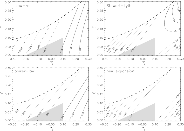
Having thus confirmed the accuracy of the code, we can compare the numerical results with those obtained from analytical approximations based on the slow-roll approximation. As input to the code we use as given by Eq. (28) and solve the perturbation equation for a range of values of and (or equivalently ) for the mode which crosses the horizon at . All higher-order are set to zero.
In Fig. 2 we display the relative differences between the numerical results and each of the four different approximations we have considered here: the lowest-order slow-roll expression, Eq. (2), the Stewart–Lyth calculation, Eq. (26), the exact power-law solution for the corresponding value of , Eq. (24), and the expansion about the power-law solution given by Eq. (31). The region above the thick dashed curve in these contour plots has been excluded, because for these values of the parameters inflation ends soon after horizon crossing and the perturbation amplitude has not attained its asymptotic value. The shaded triangle in these plots represents the region in the – plane favoured by current observations of large-scale structure and microwave background anisotropies [20], allowing for the uncertainty in cosmological parameters.
The final panel of Fig. 2 gives a comparison of the numerical results with the expansion Eq. (31) and as such requires that we know the coefficient . We have used the numerical code to evaluate this coefficient and the next-order coefficient and we find that for they are well fitted by the linear expressions
| (33) | |||||
| (34) |
As anticipated, we find the contribution from to be significantly smaller than that from .
Before we compare the numerical results with the approximations it is worth considering how representative our model is at each value of and . In other words, how reasonable is it to neglect the effect of higher-order parameters? In order to get some idea of the impact of higher-order terms on the results, we have repeated the numerical calculations for the values of and shown in Fig. 2, using a different expansion for as the input by instead expanding its logarithm:
| (36) | |||||
but keeping only the first two terms. In this case we have specific non-zero values for all of the higher-order parameters in terms of and , with for example given by
| (37) |
We therefore have numerical results for two different slices through the parameter space. Comparing the results for the two slices point-by-point in the plane we find that within the region shown in the contour plots of Fig. 2 the results differ by at most . When Eq. (34) is used to calculate the first-order correction arising from the contribution of , the relative difference between the two sets of results is found to be below within this region. Of course it will always be possible to construct models where the higher-order terms are more significant than this, but in most cases the contributions arising from the parameters beyond will be negligible.
IV Gravitational Waves
We have also carried out calculations for the somewhat simpler case of gravitational waves, where the relevant equation, analogous to Eq. (5), is [21, 8, 9]
| (38) |
The corresponding power spectrum is expanded in the same manner as for scalar perturbations
| (39) |
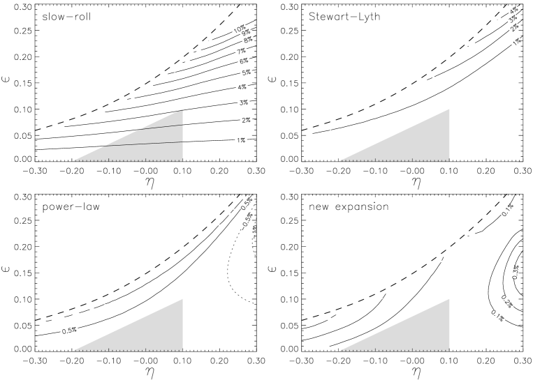
where once again is the exact power-law inflation result and the coefficients are determined from numerical calculations to be
| (40) | |||||
| (41) |
The absence of a constant term for is in agreement with the Stewart–Lyth result for the gravitational wave spectrum. The differences between this approximation and the numerical results are shown in Fig. 3, along with those for the other approximate expressions. Notice that in this case the power-law inflation result does better than the Stewart–Lyth result; this is because for gravitational waves, unlike density perturbations, the latter is simply the small parameter expansion of the former. Note also that the results for gravitational waves are much more accurate than those for density perturbations.
V Discussion
In Fig. 2 the results based on the slow-roll approximation and on the exact power-law expression are compared with the numerical results for the case of scalar perturbations. The lowest-order slow-roll result is seen to perform well only for very small values of the slow-roll parameters, with errors in excess of 10% within the observationally favoured region. In contrast, the Stewart–Lyth result fares surprisingly well. The power-law expression, although exact along the line , rapidly decreases in accuracy away from this line. By construction, our new expansion about this exact solution shows the best agreement with the numerical results across the full range of parameters, though the improvement only sets in a considerable distance from the slow-roll limit. At small and the performance of our expansion is comparable with the Stewart–Lyth calculation. These results show that the assumption , required for the Stewart–Lyth result to be applicable, doesn’t break down until well outside the region constrained by observations. It seems then that for reasonable inflationary models the Stewart–Lyth calculation works extremely well.
Fig. 3 shows the comparisons between the numerical results and each of the approximations for the spectrum of gravitational waves. In this case the exact power-law expression is found to be extremely accurate. There is considerable improvement in expanding about this exact solution, but the high level of accuracy achieved is not likely to ever be required.
As a check on the applicability of these results to general inflationary models, we have numerically evaluated the perturbation amplitude for a model with a steep polynomial potential, for the mode crossing the horizon 60 -foldings before the end of inflation. In this calculation the inputs to the numerical code are the potential and the initial conditions for the scalar field, the latter taken to be given by the inflationary attractor [18]. We took the potential
| (42) |
in order to be not too near the slow-roll limit; such potentials were discussed in Ref. [22]. The slow-roll parameters take the values
| (43) |
The comparisons between the approximations and the numerical result show a relative error
| lowest order slow-roll: | (44) | ||||
| Stewart–Lyth: | (45) | ||||
| PLI: | (46) | ||||
| new expansion: | (47) |
Note that for this case all approximation schemes fall within a 1% error.
To recap, we have used the exact power-law result as the basis for an expansion which gives the perturbation spectrum very accurately for inflationary models which are ‘close’ to power-law models, in the sense that the parameters are small. This expansion outperforms the Stewart–Lyth result for large , but within the range of values for the slow-roll parameters allowed by cosmological observations we have shown that the Stewart–Lyth result is remarkably accurate. Our results indicate that the errors in both ours and the Stewart–Lyth calculation are due mostly to neglecting terms of order , with the contributions from higher-order parameters being relatively insignificant. We stress that these conclusions are only valid if the perturbation spectrum is sensitive only to the behaviour of close to horizon crossing, but within the single scalar field paradigm we have been discussing we expect this to be the norm and the result calculated for a specific potential is consistent with this.
Acknowledgments
The authors are supported by the Royal Society. We thank Ed Copeland, Jim Lidsey and David Lyth for discussions on the analytical second-order calculation and Juan García-Bellido, Ewan Stewart and David Wands for helpful comments on this work. We acknowledge use of the Starlink computer system at the University of Sussex.
REFERENCES
- [1] M. Bersanelli et al., ESA Phase A Study document for COBRAS/SAMBA (unpublished, 1996); MAP Home Page at http://map.gsfc.nasa.gov/ (1996).
- [2] W. Hu, D. Scott, N. Sugiyama and M. White, Phys. Rev. D 52, 5498 (1995); U. Seljak and M. Zaldarriaga, MIT preprint (1996), astro-ph/9603033.
- [3] E. W. Kolb and M. S. Turner, The Early Universe, (Addison-Wesley, Redwood City, California, 1990); A. D. Linde, Particle Physics and Inflationary Cosmology (Harwood Academic, Chur, Switzerland, 1990); A. R. Liddle and D. H. Lyth, Phys. Rep. 231, 1 (1993).
- [4] A. H. Guth and S.-Y. Pi, Phys. Rev. Lett. 49, 1110 (1982); A. A. Starobinsky, Phys. Lett. 117B, 175 (1982); S. W. Hawking, Phys. Lett. 115B, 295 (1982).
- [5] J. M. Bardeen, P. J. Steinhardt and M. S. Turner, Phys. Rev. D 28, 679 (1983).
- [6] D. H. Lyth, Phys. Rev. D 31, 1792 (1985).
- [7] D. H. Lyth and E. D. Stewart, Phys. Lett. B 274, 168 (1992).
- [8] L. Abbott and M. Wise, Nucl. Phys. B244, 541 (1984).
- [9] E. D. Stewart and D. H. Lyth, Phys. Lett. B 302, 171 (1993).
- [10] J. García-Bellido and D. Wands, Sussex preprint (1996), astro-ph/9606047.
- [11] E. W. Kolb, D. S. Salopek and M. S. Turner, Phys. Rev. D 42, 3925 (1990); E. W. Kolb, Physica Scripta T36, 199 (1991).
- [12] A. D. Linde, Phys. Lett. B 259, 38 (1991), Phys. Rev D 49, 748 (1994); E. J. Copeland, A. R. Liddle, D. H. Lyth, E. D. Stewart and D. Wands, Phys. Rev D 49, 6410 (1994).
- [13] A. A. Starobinsky and J. Yokoyama, Kyoto preprint (1995), gr-qc/9502002; J. García-Bellido and D. Wands, Phys. Rev. D 52, 6739 (1995); M. Sasaki and E. D. Stewart, Prog. Theor. Phys. 95, 71 (1996); J. García-Bellido and D. Wands, Phys. Rev. D 53, 5437 (1996); T. T. Nakamura and E. D. Stewart, Tokyo preprint (1996), astro-ph/9604103.
- [14] J. E. Lidsey, A. R. Liddle, E. W. Kolb, E. J. Copeland, T. Barriero and M. Abney, Sussex preprint (1995), astro-ph/9508078.
- [15] V. F. Mukhanov, H. A. Feldman and R. H. Brandenberger, Phys. Rep. 215, 203 (1992).
- [16] V. F. Mukhanov, Pis’ma Zh. Eksp. Teor. Fiz. 41, 402 (1985) [Sov. Phys. JETP Lett. 41, 493 (1985)], Zh. Eksp. Teor. Fiz. 94, 1 (1988) [Sov. Phys. JETP 67, 1297 (1988)].
- [17] D. S. Salopek and J. R. Bond, Phys. Rev. D 42, 3936 (1990); A. G. Muslimov, Class. Quant. Grav 7, 231 (1990); J. E. Lidsey, Phys. Lett. B 273, 42 (1991).
- [18] A. R. Liddle, P. Parsons and J. D. Barrow, Phys. Rev. D 50, 7222 (1994).
- [19] R. Easther, Waseda preprint (1995), astro-ph/9511143.
- [20] A. R. Liddle, D. H. Lyth, R. K. Schaefer, Q. Shafi and P. T. P. Viana, Mon. Not. Roy. Astron. Soc. 281, 531 (1996); A. R. Liddle, D. H. Lyth, P. T. P. Viana and M. White, to appear, Mon. Not. Roy. Astron. Soc. (1996), astro-ph/9512102.
- [21] L. P. Grishchuk, Zh. Eksp. Teor. Fiz. 67, 825 (1974) [Sov. Phys. JETP 40, 409 (1974)].
- [22] G. Lazarides and Q. Shafi, Phys. Lett. B 308, 17 (1993).